Chapter 3 Preliminaries II: Data Formatting
The most merciful thing in the world, I think, is the inability of the human mind to correlate all its contents.
Note: The example code in this chapter relies on code executed in previous chapters. This code is available in a ready-to-run block in Appendix II (19.0.1).
Matrix projection models are estimated with demographic data. Regardless of whether the goal is a set of raw (empirical) or function-based matrices, the dataset used needs to follow a particular format to make the estimation of elements or vital rate models possible. Package lefko3 utilizes a standardized format similar to formats required by other protocols, such as the projection.matrix() function in package popbio. However, unlike other packages, lefko3 includes functions that can standardize a variety of starting dataset formats. These functions likely do not cover all possibilities, but deal with most of the interesting differences among the protocols that different demographers use.
The format used in analysis with lefko3 is similar to what one would expect in setting up a data frame for a linear model in R or another statistical analysis environment. If we start with a record of observations of a single individual across several years, where each observation was conducted during a single monitoring session per time interval (such as year), then our data should be formatted to allow us to assess at the very least whether the state of an individual at some time depends on the state at the previous time. For a historical model, this dependence extends one further time step back, so that we have to be able to assess demographic patterns across groups of three consecutive monitoring occasions.
In order to analyze these patterns of dependence, we break the data up into groups of two or three consecutive observation times, depending on whether the analysis will be ahistorical or historical, respectively. These broken up groups are then stacked together into a data frame. For example, if we have data for an individual in years 2010, 2011, 2012, and 2013, then we can break up these data into consecutive year pairs, starting with years 2010 and 2011, followed by years 2011 and 2012, followed by years 2012 and 2013 (if historical, then we would group together 2010-2011-2012, followed by 2011-2012-2013). In terms of the language of matrix projection models, these standardized datasets are arranged with time t followed by time t+1 if ahistorical, and time t-1, followed by time t, followed by time t+1 if in historical format. In terms of the language of linear modeling, individual status in the final time in each group can be viewed as the response variable, while status in the previous one or two times can be seen as causal. We refer to this stacked format as vertical format, because it stretches the data for a single individual vertically across data frame rows. This format can be further divided into historically-formatted vertical (hfv) format (Shefferson et al. 2021), in which groups of three consecutive monitoring times are stacked, and ahistorically-formatted vertical (ahfv) format, in which pairs of consecutive years are stacked. Note that analysis in lefko3 requires historically-formatted vertical (hfv) format.
The different aspects of the states of individuals can be described by different variables per observation time. There may be one or more measures of size, age, reproductive status, and fecundity, among other variables. Each monitoring occasion should have the same variables for use in analysis. Thus, concatenating states for consecutive pairs or triplets of occasions in this way will generally result in data frames with many more than two or three columns. Stacking the data in this fashion also typically yields multiple rows of data originating from the same individual. Until recently, these rows were typically treated as independent data points, and the simplest analyses still assume independence. However, if a separate variable is created to record the identity of the individual across rows within the dataset, then the non-independence of data points can be dealt with statistically by treating individual identity as a random factor in mixed modeling of vital rates (more on this in chapter 5).
3.1 Kinds of individual state variables that may be included
What sorts of variables can be handled in MPM analysis through lefko3? Because this package was originally developed to handle historical size-classified Lefkovitch models, it can of course handle size variables. From version 4.0.0 onward, up to three different size variables can be included in a single analysis. However, lefko3 can handle many more variables. At the very least, variables denoting reproductive status and fecundity can be included. These three groups of variables - size, reproductive status, and fecundity - are the classic three variable types used for classification purposes in stage-based models. Wildlife demographers may be more interested in age than size, and so age at each time can also be included. In fact, lefko3 automates the estimation of age and related variables, such as observed age at time t and observed lifespan, and can be used to estimate both Leslie (age-based) and age-by-stage MPMs. Plant demographers may be interested in variables denoting observation status, which is a binomial variable used to denote whether an individual is in an observable stage (lefko3 can automate the identification of these occurrences within the dataset). Some ecologists may also be interested in using multiple measures of reproductive status and fecundity, since many plants and animals have multiple modes of reproduction, and often fecundity cannot be accurately known and so must be estimated.
Identity variables may be included and used in analysis. Such variables include population identity, patch identity or subpopulation identity, individual identity, and monitoring occasion or time (denoting the time at time t). Package lefko3 can use these to subset the data accordingly, and also to estimate variables such as observed age at time t and observed lifespan. If the user has already determined stages for all individuals at all times, then these data may be incorporated as well (although lefko3 can automatically assign stages).
Demographers commonly include censoring variables to denote data points that are suspect. These can also be included in lefko3, and censored data points can also be easily removed from analysis. For example, individuals with damaged tags from which identity cannot be properly read can be marked differently in a censor variable, and analyses can then be performed with and without these potentially biasing data. Alternatively, ornithologists may mark individuals with partially missing bands with censor variables. Censor data can be added once per individual, or for each individual in each monitoring occasion.
Spatial coordinates can be included in datasets. When used, spatial coordinates should be Cartesian, and so paired as X-Y coordinates. Package lefko3 includes automated density estimation, and so these coordinates can be used to estimate spatial density.
Finally, variables can be included covering status as alive or dead, status as observed or unobserved, and up to three separate individual or environmental covariates that can be numeric or categorical. Individual covariates may be particularly useful as a means to include environmental variables, or further information on status, such as management regime or presence of injury.
3.2 Formatting demographic data properly for analysis
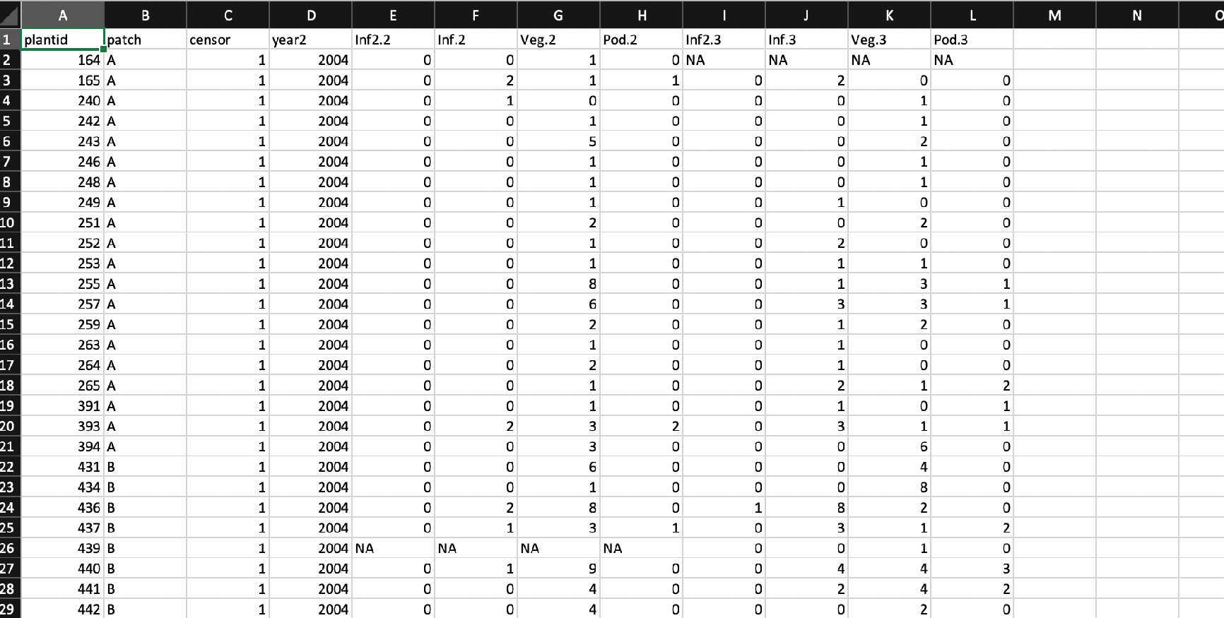
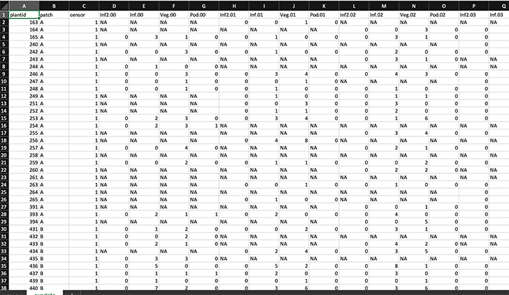
Regardless of how the dataset should be structured for analysis, demographers themselves often have their own ways of structuring data. In general, most demographers keep their data either in some variant of vertical format (explained above), or in some variant of horizontal format, in which the data for each single individual spans only a single row that contains all data on state across all monitoring occasions. In figure 3.1, we see an example of an ahistorically-formatted vertical dataset. In figure 3.2, we see an example of a horizontally-formatted dataset.
Every demographer has his or her own way of keeping data, and I personally do not feel it is up to me to judge (the level of chaos in my own record-keeping prevents me from making any harsh judgments). Therefore, lefko3 includes two powerful functions that can take most datasets falling into these two general types and standardize them into hfv format for analysis by the package. These functions are verticalize3() and historicalize3().
3.3 Function verticalize3()
Many demographers (including the author) prefer horizontal data formats for demographic record-keeping. Here, individual life histories are recorded in a spreadsheet with each unique individual’s data organized within a single row. The columns then correspond to descriptor variables and to condition at different times. This format has the advantage of making an individual’s resighting history easier to analyze even by eye, since it must occur all within a single row. In these circumstances, the verticalize3() function can standardize these data into hfv format.
Function verticalize3() takes a number of inputs. Naturally, it needs the data frame being used for analysis (the data field). It also requires input corresponding to the number of monitoring occasions that the dataset covers (field noyears), and which columns identify the population, patch or subpopulation, and individual (fields popidcol, patchidcol, and individcol, respectively).
After these most basic of fields have been entered, the columns conveying each kind of demographic variable need to be identified (this is a very flexible function, so only those variables that actually occur in the dataset need be identified and all others can be ignored). Up to three separate size variables can be identified (sizeacol, sizebcol, and sizeccol), as can up to two reproductive status variables (repstracol and restrbcol), and up to two fecundity variables (fecacol and fecbcol). These variables will naturally repeat across monitoring occasions, and so each variable represents as many actual columns as monitoring occasions covered by the dataset.
To ensure that R finds all columns corresponding to a variable, the user may take one of two approaches. The most flexible is to treat each input field as a vector, and to input the name or column number of each variable in order of monitoring occasion. For example, if we decided to use only one size variable, perhaps the height of a plant in centimeters, and this variable is labelled ht.2010, ht.2011, ht.2012, and ht.2013 for the years 2010, 2011, 2012, and 2013, then we can input the following.
sizeacol = c("ht.2010", "ht.2011", "ht.2012", "ht.2013").
All other variables covering status across time can be input in the same way, yielding equal length vectors in the same temporal order.
Alternatively, if the data are arranged such that each monitoring occasion has its variables arranged in a strictly repeating order, then we can use the blocksize argument to simplify our function call. Here, each variable in our dataset should be a fixed number of columns away from the equivalent variable in the preceding time and in the next time. Then, only the first column of each core variable group needs to be designated in verticalize3(), and the blocksize field can be set to the number of columns separating these entries. In the plant height example, if each size variable is 10 columns after the previous size variable and this pattern holds for all other variable types, then this would mean entering only the following.
noyears = 4, blocksize = 10, sizeacol = "ht.2010"
Note that the use of the blocksize option absolutely requires that each variable group occurs exactly blocksize columns after the previous instance, with absolutely no exceptions other than the first instance. Users who occasionally add empty or extra columns here and there in their dataset will find mistakes in the resulting standardization if they do not make sure that the exact number of columns between instances is always the same.
While standardizing the data, function verticalize3() can also assign stage designations if given a proper stageframe (the stageassign field). For this purpose, lefko3 also needs the proper size variable designations. Currently, the options include:
sizea,sizeb, orsizecif only one of these size metrics determines stagesizeab,sizeac, orsizebcif stage assignment is based on a pair of size metricssizeabcif stage assignment should utilize three size metrics; orsizeadded, if stage assignment should proceed on the basis of the sum of all used size metrics.
Stage assignment is automated using these size metrics as well as reproductive status, observation status, and status as propagule, immature, and mature. Stage assignment will yield warnings and unassigned stages if any combination of variables is found in the demographic dataset that does not fit exactly one stage in the stage frame. We also encourage the use of this function without stage assignment on the first pass, since this will allow users to explore the data more fully prior to the development of a life history model and stageframe.
Function verticalize3() includes a few more fields of interest. The repstrrel and fecrel fields provide means of equalizing reproductive status variables and fecundity variables, respectively, that are set on different scales. For example, if two reproductive status variables are used, the first covering the presence of single-flowered stems and the second covering the presence of double-flowered stems, then setting repstrrel = 2 will tell R that the second variable counts for twice the reproductive status of the first. The same applies to fecundity with the fecrel field, if two different fecundity measures are used.
Demographers using censoring variables will find powerful options in this function. First, censorcol can be set to a static censor variable covering an individual’s entire resighting history, or to censor variables that vary across time. This can be set with the censorRepeat field, which defaults to FALSE and so assumes that censor values do not vary across time. The value of the censor variable used to denote which individuals to keep can be set to any numeric value (the censorkeep option). The default is censorkeep = 0, meaning that any data points marked 0 are considered OK and kept, while any other value is assumed to be subject to removal. Any character or numeric value may be used to mark data to keep, even NA. Finally, if all options are set as described, then function verticalize3() will format the data with censor variables in place but will not remove any data points. To force verticalize3() to remove censored data points, set censor = TRUE (the default is censor = FALSE).
Function verticalize3() can handle spatial coordinates, and can even estimate spatial density. Cartesian coordinates for each individual are assumed to be a single set. However, if coordinates can change across time and each time point has its own set of coordinates for each individual present, then users can set coordsRepeat = TRUE. If the intent in using these coordinates is to estimate spatial density, then this function will calculate the number of individuals within some radius of each focal individual in each monitoring time if given the length of the radius to use via option spacing (e.g. spacing = 1 sets the distance radius to check for other individuals nearby at one unit of distance).
This function includes further parameters handling miscellaneous cases. First, demographers often treat missing data as blanks within their spreadsheets. Setting NAas0 = TRUE tells R to interpret missing data as zeros. This can be useful in many circumstances. For example, if fecundity is estimated as the number of flowers per individual in a plant demographic study, but the number of flowers per individual is only recorded if flowers actually exist, then setting NAas0 = TRUE can allow 0 values to be incorporated in analyses of fecundity when no data were entered for flower number. Second, the NRasRep option allows stage classification to proceed without matching stage reproductive characteristics to the data. For example, if stages are defined such that mature stages are reproductive but it is nonetheless possible for fecundity to equal 0, then setting NRasRep = TRUE tells R not to use reproductive status in stage classification. Otherwise, R will assume that a mature individual that produces offspring is in a different stage than a mature individual that does not. Third, the NAasObs option provides a means of telling R that unobservable stages should be treated as observed during stage classification, if set to TRUE (the default is FALSE). Fourth, the reduce option, if set to TRUE, will tell R that any columns in the output dataset with a single constant value across all rows should be removed, as invariant variables yield no influence on response variables in statistical modeling. Fifth, the a2check field should generally be kept to FALSE (the default), but if set to TRUE, then the resulting standardized dataset will include data for individuals not alive in time t (these instances are removed automatically under the default, since it is only individuals alive in time t that can transition to anything in time t+1). This function also assumes that monitoring studies are conducted using pre-breeding life history models, making 1 the earliest observed age. To use a post-breeding model, set prebreeding = FALSE. Finally, the age_offset option can be used to add a specific number to all ages, as might happen if the first few years of life cannot be monitored.
3.3.1 An example of verticalize3()
Now that we have explained the options, let’s standardize data frames for the stageframes created in the last chapter (chapter 2). Let’s first standardize the vertical dataset for the raw MPM. Because we are lumping reproductive and non-reproductive individuals into the non-dormant adult classes, we will set NRasRep = TRUE. Otherwise, verticalize3() will attempt to use the reproductive status of individuals in classification, and will fail due to the presence of non-reproductive adults. We will also set NAas0 = TRUE to make sure that NA values in size are turned into 0 entries where necessary, and so aid in the assignment of the vegetative dormancy stage. Note that we will set up three different size variables here, as sizea, sizeb, and sizec, and that we will tell R that we want overall stage classification size to be the sum of these (stagesize = "sizeadded"). Finally, since the individuals in this dataset must be at least 5 years old when they are first seen as adults, we will use the age_offset option to adjust the estimated age.
cypraw_v1 <- verticalize3(data = cypdata, noyears = 6, firstyear = 2004,
  patchidcol = "patch", individcol = "plantid", blocksize = 4,
  sizeacol = "Inf2.04", sizebcol = "Inf.04", sizeccol = "Veg.04",
  repstracol = "Inf.04", repstrbcol = "Inf2.04", fecacol = "Pod.04",
  stageassign = cypframe_raw, stagesize = "sizeadded", NAas0 = TRUE,
  NRasRep = TRUE, age_offset = 4)
Let’s now take a look at a summary of this dataset. We have two options for this. First, we could use R’s summary() function, which would treat our new historically vertically (hfv) formatted dataset as a standard data frame and use the standard summary procedure for data frames. Or, we may use lefko3’s summary_hfv() function, which gives us a little extra information.
summary_hfv(cypraw_v1, full = TRUE)
>
> This hfv dataset contains 320 rows, 57 variables, 1 population,
> 3 patches, 74 individuals, and 5 time steps.
>      rowid          popid           patchid    individ           year2
>  Min.   : 1.00   Length:320         A: 93   Min.   : 164.0   Min.   :2004
>  1st Qu.:21.00   Class :character   B:154   1st Qu.: 391.0   1st Qu.:2005
>  Median :37.50   Mode  :character   C: 73   Median : 453.0   Median :2006
>  Mean   :38.45                              Mean   : 651.5   Mean   :2006
>  3rd Qu.:56.00                              3rd Qu.: 476.0   3rd Qu.:2007
>  Max.   :77.00                              Max.   :1560.0   Max.   :2008
>    firstseen       lastseen        obsage       obslifespan
>  Min.   :2004   Min.   :2004   Min.   :5.000   Min.   :0.000
>  1st Qu.:2004   1st Qu.:2009   1st Qu.:6.000   1st Qu.:5.000
>  Median :2004   Median :2009   Median :7.000   Median :5.000
>  Mean   :2004   Mean   :2009   Mean   :6.853   Mean   :4.556
>  3rd Qu.:2004   3rd Qu.:2009   3rd Qu.:8.000   3rd Qu.:5.000
>  Max.   :2008   Max.   :2009   Max.   :9.000   Max.   :5.000
>      sizea1             sizeb1            sizec1       size1added
>  Min.   :0.000000   Min.   : 0.0000   Min.   : 0.0   Min.   : 0.000
>  1st Qu.:0.000000   1st Qu.: 0.0000   1st Qu.: 0.0   1st Qu.: 0.000
>  Median :0.000000   Median : 0.0000   Median : 1.0   Median : 2.000
>  Mean   :0.009375   Mean   : 0.7469   Mean   : 1.9   Mean   : 2.656
>  3rd Qu.:0.000000   3rd Qu.: 1.0000   3rd Qu.: 3.0   3rd Qu.: 4.000
>  Max.   :1.000000   Max.   :18.0000   Max.   :13.0   Max.   :21.000
>     repstra1          repstrb1         repstr1added         feca1
>  Min.   : 0.0000   Min.   :0.000000   Min.   : 0.0000   Min.   :0.0000
>  1st Qu.: 0.0000   1st Qu.:0.000000   1st Qu.: 0.0000   1st Qu.:0.0000
>  Median : 0.0000   Median :0.000000   Median : 0.0000   Median :0.0000
>  Mean   : 0.7469   Mean   :0.009375   Mean   : 0.7562   Mean   :0.2656
>  3rd Qu.: 1.0000   3rd Qu.:0.000000   3rd Qu.: 1.0000   3rd Qu.:0.0000
>  Max.   :18.0000   Max.   :1.000000   Max.   :18.0000   Max.   :7.0000
>    fec1added        obsstatus1       repstatus1       fecstatus1
>  Min.   :0.0000   Min.   :0.0000   Min.   :0.0000   Min.   :0.0000
>  1st Qu.:0.0000   1st Qu.:0.0000   1st Qu.:0.0000   1st Qu.:0.0000
>  Median :0.0000   Median :1.0000   Median :0.0000   Median :0.0000
>  Mean   :0.2656   Mean   :0.7469   Mean   :0.2875   Mean   :0.1344
>  3rd Qu.:0.0000   3rd Qu.:1.0000   3rd Qu.:1.0000   3rd Qu.:0.0000
>  Max.   :7.0000   Max.   :1.0000   Max.   :1.0000   Max.   :1.0000
>    matstatus1         alive1          stage1           stage1index
>  Min.   :0.0000   Min.   :0.0000   Length:320         Min.   : 0.000
>  1st Qu.:1.0000   1st Qu.:1.0000   Class :character   1st Qu.: 6.000
>  Median :1.0000   Median :1.0000   Mode  :character   Median : 8.000
>  Mean   :0.7688   Mean   :0.7688                      Mean   : 6.144
>  3rd Qu.:1.0000   3rd Qu.:1.0000                      3rd Qu.: 8.000
>  Max.   :1.0000   Max.   :1.0000                      Max.   :11.000
>      sizea2             sizeb2            sizec2         size2added
>  Min.   :0.000000   Min.   : 0.0000   Min.   : 0.000   Min.   : 0.000
>  1st Qu.:0.000000   1st Qu.: 0.0000   1st Qu.: 1.000   1st Qu.: 1.000
>  Median :0.000000   Median : 0.0000   Median : 2.000   Median : 2.000
>  Mean   :0.009375   Mean   : 0.8969   Mean   : 2.416   Mean   : 3.322
>  3rd Qu.:0.000000   3rd Qu.: 1.0000   3rd Qu.: 3.000   3rd Qu.: 4.000
>  Max.   :1.000000   Max.   :18.0000   Max.   :13.000   Max.   :24.000
>     repstra2          repstrb2         repstr2added         feca2
>  Min.   : 0.0000   Min.   :0.000000   Min.   : 0.0000   Min.   :0.0000
>  1st Qu.: 0.0000   1st Qu.:0.000000   1st Qu.: 0.0000   1st Qu.:0.0000
>  Median : 0.0000   Median :0.000000   Median : 0.0000   Median :0.0000
>  Mean   : 0.8969   Mean   :0.009375   Mean   : 0.9062   Mean   :0.2906
>  3rd Qu.: 1.0000   3rd Qu.:0.000000   3rd Qu.: 1.0000   3rd Qu.:0.0000
>  Max.   :18.0000   Max.   :1.000000   Max.   :18.0000   Max.   :7.0000
>    fec2added        obsstatus2       repstatus2       fecstatus2
>  Min.   :0.0000   Min.   :0.0000   Min.   :0.0000   Min.   :0.0000
>  1st Qu.:0.0000   1st Qu.:1.0000   1st Qu.:0.0000   1st Qu.:0.0000
>  Median :0.0000   Median :1.0000   Median :0.0000   Median :0.0000
>  Mean   :0.2906   Mean   :0.9531   Mean   :0.3688   Mean   :0.1562
>  3rd Qu.:0.0000   3rd Qu.:1.0000   3rd Qu.:1.0000   3rd Qu.:0.0000
>  Max.   :7.0000   Max.   :1.0000   Max.   :1.0000   Max.   :1.0000
>    matstatus2     alive2     stage2           stage2index
>  Min.   :1    Min.   :1   Length:320         Min.   : 6.000
>  1st Qu.:1    1st Qu.:1   Class :character   1st Qu.: 7.000
>  Median :1    Median :1   Mode  :character   Median : 8.000
>  Mean   :1    Mean   :1                      Mean   : 7.919
>  3rd Qu.:1    3rd Qu.:1                      3rd Qu.: 8.000
>  Max.   :1    Max.   :1                      Max.   :11.000
>      sizea3             sizeb3           sizec3         size3added
>  Min.   :0.000000   Min.   : 0.000   Min.   : 0.000   Min.   : 0.000
>  1st Qu.:0.000000   1st Qu.: 0.000   1st Qu.: 1.000   1st Qu.: 1.000
>  Median :0.000000   Median : 0.000   Median : 1.000   Median : 2.000
>  Mean   :0.009375   Mean   : 1.069   Mean   : 2.209   Mean   : 3.288
>  3rd Qu.:0.000000   3rd Qu.: 1.000   3rd Qu.: 3.000   3rd Qu.: 4.000
>  Max.   :1.000000   Max.   :18.000   Max.   :13.000   Max.   :24.000
>     repstra3         repstrb3         repstr3added        feca3
>  Min.   : 0.000   Min.   :0.000000   Min.   : 0.000   Min.   :0.0000
>  1st Qu.: 0.000   1st Qu.:0.000000   1st Qu.: 0.000   1st Qu.:0.0000
>  Median : 0.000   Median :0.000000   Median : 0.000   Median :0.0000
>  Mean   : 1.069   Mean   :0.009375   Mean   : 1.078   Mean   :0.4562
>  3rd Qu.: 1.000   3rd Qu.:0.000000   3rd Qu.: 1.000   3rd Qu.:0.0000
>  Max.   :18.000   Max.   :1.000000   Max.   :18.000   Max.   :8.0000
>    fec3added        obsstatus3    repstatus3    fecstatus3       matstatus3
>  Min.   :0.0000   Min.   :0.0   Min.   :0.0   Min.   :0.0000   Min.   :1
>  1st Qu.:0.0000   1st Qu.:1.0   1st Qu.:0.0   1st Qu.:0.0000   1st Qu.:1
>  Median :0.0000   Median :1.0   Median :0.0   Median :0.0000   Median :1
>  Mean   :0.4562   Mean   :0.9   Mean   :0.4   Mean   :0.2219   Mean   :1
>  3rd Qu.:0.0000   3rd Qu.:1.0   3rd Qu.:1.0   3rd Qu.:0.0000   3rd Qu.:1
>  Max.   :8.0000   Max.   :1.0   Max.   :1.0   Max.   :1.0000   Max.   :1
>      alive3          stage3           stage3index
>  Min.   :0.0000   Length:320         Min.   : 0.000
>  1st Qu.:1.0000   Class :character   1st Qu.: 7.000
>  Median :1.0000   Mode  :character   Median : 8.000
>  Mean   :0.9469                      Mean   : 7.544
>  3rd Qu.:1.0000                      3rd Qu.: 8.000
>  Max.   :1.0000                      Max.   :11.000
In the summary of the resulting data frame, we first see that there are 320 rows, 57 variables, one population, three patches, 74 individuals, and 5 time steps. This information gives us a good understanding of the dimensions of the dataset. This is followed by R’s data frame summary, where we see that the first four variables are identifying information - they show the data row (rowid), the population ID (popid), the patch ID (patchid), and the individual ID (individ), in order. These are followed by year at time t (year2), followed by two variables identifying in what monitoring occasion the individual was first seen (firstseen), and in what occasion it was last seen (lastseen). The next variable, obsage, gives the estimated age at time t. The next variable, obslifespan, gives the full length of time that the individual was observed in the dataset. After that, we see a group of 15 variables typically ending with the number 1. These 15 variables correspond to the state of each individual in time t-1 (generally referred to as time1 in the actual code). Similarly, the next 15 variables typically end with the number 2 and represent state in time t, while the last 15 variables typically end in the number 3 and refer to state in time t+1. Most of these variables should be obvious to interpret given the names (definitions are in the help file for this function). Note that the final seven variables in each group are calculated by verticalize3(). These variables represent observation status, reproductive status, fecundity status, maturity status, status as alive or dead, stage name, and stage number (with reference to the stageframe), in order.
The summary_hfv() function can also produce just the initial dimensional output, as below.
summary_hfv(cypraw_v1)
>
> This hfv dataset contains 320 rows, 57 variables, 1 population,
> 3 patches, 74 individuals, and 5 time steps.
Let’s also create our standardized data frame for the function-based MPM, as below. Remember that some of the settings need to change here because we will use a different life history model. Particularly, we are now going to separate adults not just by size but by reproductive status. So, we will not set NRasRep = TRUE here (the default is NRasRep = FALSE).
cypfb_v1 <- verticalize3(data = cypdata, noyears = 6, firstyear = 2004,
  patchidcol = "patch", individcol = "plantid", blocksize = 4,
  sizeacol = "Inf2.04", sizebcol = "Inf.04", sizeccol = "Veg.04",
  repstracol = "Inf.04", repstrbcol = "Inf2.04", fecacol = "Pod.04",
  stageassign = cypframe_fb, stagesize = "sizeadded", NAas0 = TRUE,
  age_offset = 4)

summary_hfv(cypfb_v1, full = TRUE)
>
> This hfv dataset contains 320 rows, 57 variables, 1 population,
> 3 patches, 74 individuals, and 5 time steps.
>      rowid          popid           patchid    individ           year2
>  Min.   : 1.00   Length:320         A: 93   Min.   : 164.0   Min.   :2004
>  1st Qu.:21.00   Class :character   B:154   1st Qu.: 391.0   1st Qu.:2005
>  Median :37.50   Mode  :character   C: 73   Median : 453.0   Median :2006
>  Mean   :38.45                              Mean   : 651.5   Mean   :2006
>  3rd Qu.:56.00                              3rd Qu.: 476.0   3rd Qu.:2007
>  Max.   :77.00                              Max.   :1560.0   Max.   :2008
>    firstseen       lastseen        obsage       obslifespan
>  Min.   :2004   Min.   :2004   Min.   :5.000   Min.   :0.000
>  1st Qu.:2004   1st Qu.:2009   1st Qu.:6.000   1st Qu.:5.000
>  Median :2004   Median :2009   Median :7.000   Median :5.000
>  Mean   :2004   Mean   :2009   Mean   :6.853   Mean   :4.556
>  3rd Qu.:2004   3rd Qu.:2009   3rd Qu.:8.000   3rd Qu.:5.000
>  Max.   :2008   Max.   :2009   Max.   :9.000   Max.   :5.000
>      sizea1             sizeb1            sizec1       size1added
>  Min.   :0.000000   Min.   : 0.0000   Min.   : 0.0   Min.   : 0.000
>  1st Qu.:0.000000   1st Qu.: 0.0000   1st Qu.: 0.0   1st Qu.: 0.000
>  Median :0.000000   Median : 0.0000   Median : 1.0   Median : 2.000
>  Mean   :0.009375   Mean   : 0.7469   Mean   : 1.9   Mean   : 2.656
>  3rd Qu.:0.000000   3rd Qu.: 1.0000   3rd Qu.: 3.0   3rd Qu.: 4.000
>  Max.   :1.000000   Max.   :18.0000   Max.   :13.0   Max.   :21.000
>     repstra1          repstrb1         repstr1added         feca1
>  Min.   : 0.0000   Min.   :0.000000   Min.   : 0.0000   Min.   :0.0000
>  1st Qu.: 0.0000   1st Qu.:0.000000   1st Qu.: 0.0000   1st Qu.:0.0000
>  Median : 0.0000   Median :0.000000   Median : 0.0000   Median :0.0000
>  Mean   : 0.7469   Mean   :0.009375   Mean   : 0.7562   Mean   :0.2656
>  3rd Qu.: 1.0000   3rd Qu.:0.000000   3rd Qu.: 1.0000   3rd Qu.:0.0000
>  Max.   :18.0000   Max.   :1.000000   Max.   :18.0000   Max.   :7.0000
>    fec1added        obsstatus1       repstatus1       fecstatus1
>  Min.   :0.0000   Min.   :0.0000   Min.   :0.0000   Min.   :0.0000
>  1st Qu.:0.0000   1st Qu.:0.0000   1st Qu.:0.0000   1st Qu.:0.0000
>  Median :0.0000   Median :1.0000   Median :0.0000   Median :0.0000
>  Mean   :0.2656   Mean   :0.7469   Mean   :0.2875   Mean   :0.1344
>  3rd Qu.:0.0000   3rd Qu.:1.0000   3rd Qu.:1.0000   3rd Qu.:0.0000
>  Max.   :7.0000   Max.   :1.0000   Max.   :1.0000   Max.   :1.0000
>    matstatus1         alive1          stage1           stage1index
>  Min.   :0.0000   Min.   :0.0000   Length:320         Min.   : 0.00
>  1st Qu.:1.0000   1st Qu.:1.0000   Class :character   1st Qu.: 6.00
>  Median :1.0000   Median :1.0000   Mode  :character   Median : 8.00
>  Mean   :0.7688   Mean   :0.7688                      Mean   :14.17
>  3rd Qu.:1.0000   3rd Qu.:1.0000                      3rd Qu.:31.00
>  Max.   :1.0000   Max.   :1.0000                      Max.   :51.00
>      sizea2             sizeb2            sizec2         size2added
>  Min.   :0.000000   Min.   : 0.0000   Min.   : 0.000   Min.   : 0.000
>  1st Qu.:0.000000   1st Qu.: 0.0000   1st Qu.: 1.000   1st Qu.: 1.000
>  Median :0.000000   Median : 0.0000   Median : 2.000   Median : 2.000
>  Mean   :0.009375   Mean   : 0.8969   Mean   : 2.416   Mean   : 3.322
>  3rd Qu.:0.000000   3rd Qu.: 1.0000   3rd Qu.: 3.000   3rd Qu.: 4.000
>  Max.   :1.000000   Max.   :18.0000   Max.   :13.000   Max.   :24.000
>     repstra2          repstrb2         repstr2added         feca2
>  Min.   : 0.0000   Min.   :0.000000   Min.   : 0.0000   Min.   :0.0000
>  1st Qu.: 0.0000   1st Qu.:0.000000   1st Qu.: 0.0000   1st Qu.:0.0000
>  Median : 0.0000   Median :0.000000   Median : 0.0000   Median :0.0000
>  Mean   : 0.8969   Mean   :0.009375   Mean   : 0.9062   Mean   :0.2906
>  3rd Qu.: 1.0000   3rd Qu.:0.000000   3rd Qu.: 1.0000   3rd Qu.:0.0000
>  Max.   :18.0000   Max.   :1.000000   Max.   :18.0000   Max.   :7.0000
>    fec2added        obsstatus2       repstatus2       fecstatus2
>  Min.   :0.0000   Min.   :0.0000   Min.   :0.0000   Min.   :0.0000
>  1st Qu.:0.0000   1st Qu.:1.0000   1st Qu.:0.0000   1st Qu.:0.0000
>  Median :0.0000   Median :1.0000   Median :0.0000   Median :0.0000
>  Mean   :0.2906   Mean   :0.9531   Mean   :0.3688   Mean   :0.1562
>  3rd Qu.:0.0000   3rd Qu.:1.0000   3rd Qu.:1.0000   3rd Qu.:0.0000
>  Max.   :7.0000   Max.   :1.0000   Max.   :1.0000   Max.   :1.0000
>    matstatus2     alive2     stage2           stage2index        sizea3
>  Min.   :1    Min.   :1   Length:320         Min.   : 6.00   Min.   :0.000000
>  1st Qu.:1    1st Qu.:1   Class :character   1st Qu.: 7.00   1st Qu.:0.000000
>  Median :1    Median :1   Mode  :character   Median :10.00   Median :0.000000
>  Mean   :1    Mean   :1                      Mean   :18.17   Mean   :0.009375
>  3rd Qu.:1    3rd Qu.:1                      3rd Qu.:32.00   3rd Qu.:0.000000
>  Max.   :1    Max.   :1                      Max.   :54.00   Max.   :1.000000
>      sizeb3           sizec3         size3added        repstra3
>  Min.   : 0.000   Min.   : 0.000   Min.   : 0.000   Min.   : 0.000
>  1st Qu.: 0.000   1st Qu.: 1.000   1st Qu.: 1.000   1st Qu.: 0.000
>  Median : 0.000   Median : 1.000   Median : 2.000   Median : 0.000
>  Mean   : 1.069   Mean   : 2.209   Mean   : 3.288   Mean   : 1.069
>  3rd Qu.: 1.000   3rd Qu.: 3.000   3rd Qu.: 4.000   3rd Qu.: 1.000
>  Max.   :18.000   Max.   :13.000   Max.   :24.000   Max.   :18.000
>     repstrb3         repstr3added        feca3          fec3added
>  Min.   :0.000000   Min.   : 0.000   Min.   :0.0000   Min.   :0.0000
>  1st Qu.:0.000000   1st Qu.: 0.000   1st Qu.:0.0000   1st Qu.:0.0000
>  Median :0.000000   Median : 0.000   Median :0.0000   Median :0.0000
>  Mean   :0.009375   Mean   : 1.078   Mean   :0.4562   Mean   :0.4562
>  3rd Qu.:0.000000   3rd Qu.: 1.000   3rd Qu.:0.0000   3rd Qu.:0.0000
>  Max.   :1.000000   Max.   :18.000   Max.   :8.0000   Max.   :8.0000
>    obsstatus3    repstatus3    fecstatus3       matstatus3     alive3
>  Min.   :0.0   Min.   :0.0   Min.   :0.0000   Min.   :1    Min.   :0.0000
>  1st Qu.:1.0   1st Qu.:0.0   1st Qu.:0.0000   1st Qu.:1    1st Qu.:1.0000
>  Median :1.0   Median :0.0   Median :0.0000   Median :1    Median :1.0000
>  Mean   :0.9   Mean   :0.4   Mean   :0.2219   Mean   :1    Mean   :0.9469
>  3rd Qu.:1.0   3rd Qu.:1.0   3rd Qu.:0.0000   3rd Qu.:1    3rd Qu.:1.0000
>  Max.   :1.0   Max.   :1.0   Max.   :1.0000   Max.   :1    Max.   :1.0000
>     stage3           stage3index
>  Length:320         Min.   : 0.00
>  Class :character   1st Qu.: 7.00
>  Mode  :character   Median :10.00
>                     Mean   :18.57
>                     3rd Qu.:33.00
>                     Max.   :54.00
The output dataset includes a number of summary variables, but the data is essentially broken down into groups of three consecutive monitoring occasions each (occasions t+1, t, and t-1, corresponding to year3, year2, and year1 in the output, respectively), with individuals spread across multiple rows. The output dataset is further limited to those entries in which the individual is alive in occasion t (year2), meaning that all rows in which an individual is dead or not yet recruited in occasion t are dropped. Since the input data is the same, we should see the same numbers of rows and columns in the raw and function-based cases, regardless of the different stageframes used. Thus, we have 320 rows of data and 57 variables in the raw case, and 320 rows of data and 57 variables in the function-based case.
3.4 Function historicalize3()
What should be done if the dataset is in ahistorical vertical format, in which an individual’s condition across time is recorded across rows in a spreadsheet, with a single row corresponding to either a single observation or to a pair of consecutive observations? In that case, the historicalize3() function can standardize the dataset properly. The inputs to this function are very similar to verticalize3(). However, the historicalize3() function assumes that the input dataset is organized with rows corresponding to individual status in either only one monitoring occasion, or two consecutive occasions. Inputs include a series of variables more or less equivalent to input options in verticalize3(), but some variable names end with 2col, and others end with 3col. The former variables denote status in time t, and are the minimum required for this function to run. If each row includes status in paired consecutive times, then variables ending in 3col can be used to designate status in time t+1. Additionally, this function requires a single variable identifying individuals across rows (individcol), so that each individual’s resighting history can be inferred and each group of three consecutive monitoring times can be put together. All other fields work essentially the same as in verticalize3().
3.4.1 An example of historicalize3()
Package lefko3 also includes dataset cypvert, which is the same dataset as cypdata but set in ahistorical vertical format. Here, we will use the historicalize3() function to standardize this dataset, using the plantid variable as the individual identity term.
data(cypvert)

cypraw_v2 <- historicalize3(data = cypvert, patchidcol = "patch",
  individcol = "plantid", year2col = "year2", sizea2col = "Inf2.2",
  sizea3col = "Inf2.3", sizeb2col = "Inf.2", sizeb3col = "Inf.3",
  sizec2col = "Veg.2", sizec3col = "Veg.3", repstra2col = "Inf2.2",
  repstra3col = "Inf2.3", repstrb2col = "Inf.2", repstrb3col = "Inf.3",
  feca2col = "Pod.2", feca3col = "Pod.3", repstrrel = 2,
  stageassign = cypframe_raw, stagesize = "sizeadded", censorcol = "censor",
  censorkeep = 1, censor = FALSE, NAas0 = TRUE, NRasRep = TRUE, age_offset = 4,
  reduce = TRUE)

summary_hfv(cypraw_v2, full = TRUE)
>
> This hfv dataset contains 320 rows, 57 variables, 1 population,
> 3 patches, 74 individuals, and 5 time steps.
>      rowid           popid           patchid    individ           year2
>  Min.   :  0.00   Length:320         A: 93   Min.   : 164.0   Min.   :2004
>  1st Qu.: 79.75   Class :character   B:154   1st Qu.: 391.0   1st Qu.:2005
>  Median :159.50   Mode  :character   C: 73   Median : 453.0   Median :2006
>  Mean   :159.70                              Mean   : 651.5   Mean   :2006
>  3rd Qu.:239.25                              3rd Qu.: 476.0   3rd Qu.:2007
>  Max.   :321.00                              Max.   :1560.0   Max.   :2008
>    firstseen       lastseen        obsage       obslifespan
>  Min.   :2004   Min.   :2004   Min.   :5.000   Min.   :0.000
>  1st Qu.:2004   1st Qu.:2009   1st Qu.:6.000   1st Qu.:5.000
>  Median :2004   Median :2009   Median :7.000   Median :5.000
>  Mean   :2004   Mean   :2009   Mean   :6.853   Mean   :4.556
>  3rd Qu.:2004   3rd Qu.:2009   3rd Qu.:8.000   3rd Qu.:5.000
>  Max.   :2008   Max.   :2009   Max.   :9.000   Max.   :5.000
>      sizea1             sizeb1            sizec1       size1added
>  Min.   :0.000000   Min.   : 0.0000   Min.   : 0.0   Min.   : 0.000
>  1st Qu.:0.000000   1st Qu.: 0.0000   1st Qu.: 0.0   1st Qu.: 0.000
>  Median :0.000000   Median : 0.0000   Median : 1.0   Median : 2.000
>  Mean   :0.009375   Mean   : 0.7469   Mean   : 1.9   Mean   : 2.656
>  3rd Qu.:0.000000   3rd Qu.: 1.0000   3rd Qu.: 3.0   3rd Qu.: 4.000
>  Max.   :1.000000   Max.   :18.0000   Max.   :13.0   Max.   :21.000
>     repstra1           repstrb1        repstr1added        feca1
>  Min.   :0.000000   Min.   : 0.0000   Min.   : 0.000   Min.   :0.0000
>  1st Qu.:0.000000   1st Qu.: 0.0000   1st Qu.: 0.000   1st Qu.:0.0000
>  Median :0.000000   Median : 0.0000   Median : 0.000   Median :0.0000
>  Mean   :0.009375   Mean   : 0.7469   Mean   : 1.503   Mean   :0.2656
>  3rd Qu.:0.000000   3rd Qu.: 1.0000   3rd Qu.: 2.000   3rd Qu.:0.0000
>  Max.   :1.000000   Max.   :18.0000   Max.   :36.000   Max.   :7.0000
>    fec1added        obsstatus1       repstatus1       fecstatus1
>  Min.   :0.0000   Min.   :0.0000   Min.   :0.0000   Min.   :0.0000
>  1st Qu.:0.0000   1st Qu.:0.0000   1st Qu.:0.0000   1st Qu.:0.0000
>  Median :0.0000   Median :1.0000   Median :0.0000   Median :0.0000
>  Mean   :0.2656   Mean   :0.7469   Mean   :0.2875   Mean   :0.1344
>  3rd Qu.:0.0000   3rd Qu.:1.0000   3rd Qu.:1.0000   3rd Qu.:0.0000
>  Max.   :7.0000   Max.   :1.0000   Max.   :1.0000   Max.   :1.0000
>    matstatus1         alive1          stage1           stage1index
>  Min.   :0.0000   Min.   :0.0000   Length:320         Min.   : 0.000
>  1st Qu.:1.0000   1st Qu.:1.0000   Class :character   1st Qu.: 6.000
>  Median :1.0000   Median :1.0000   Mode  :character   Median : 8.000
>  Mean   :0.7688   Mean   :0.7688                      Mean   : 6.144
>  3rd Qu.:1.0000   3rd Qu.:1.0000                      3rd Qu.: 8.000
>  Max.   :1.0000   Max.   :1.0000                      Max.   :11.000
>      sizea2             sizeb2            sizec2         size2added
>  Min.   :0.000000   Min.   : 0.0000   Min.   : 0.000   Min.   : 0.000
>  1st Qu.:0.000000   1st Qu.: 0.0000   1st Qu.: 1.000   1st Qu.: 1.000
>  Median :0.000000   Median : 0.0000   Median : 2.000   Median : 2.000
>  Mean   :0.009375   Mean   : 0.8969   Mean   : 2.416   Mean   : 3.322
>  3rd Qu.:0.000000   3rd Qu.: 1.0000   3rd Qu.: 3.000   3rd Qu.: 4.000
>  Max.   :1.000000   Max.   :18.0000   Max.   :13.000   Max.   :24.000
>     repstra2           repstrb2        repstr2added        feca2
>  Min.   :0.000000   Min.   : 0.0000   Min.   : 0.000   Min.   :0.0000
>  1st Qu.:0.000000   1st Qu.: 0.0000   1st Qu.: 0.000   1st Qu.:0.0000
>  Median :0.000000   Median : 0.0000   Median : 0.000   Median :0.0000
>  Mean   :0.009375   Mean   : 0.8969   Mean   : 1.803   Mean   :0.2906
>  3rd Qu.:0.000000   3rd Qu.: 1.0000   3rd Qu.: 2.000   3rd Qu.:0.0000
>  Max.   :1.000000   Max.   :18.0000   Max.   :36.000   Max.   :7.0000
>    fec2added        obsstatus2       repstatus2       fecstatus2
>  Min.   :0.0000   Min.   :0.0000   Min.   :0.0000   Min.   :0.0000
>  1st Qu.:0.0000   1st Qu.:1.0000   1st Qu.:0.0000   1st Qu.:0.0000
>  Median :0.0000   Median :1.0000   Median :0.0000   Median :0.0000
>  Mean   :0.2906   Mean   :0.9531   Mean   :0.3688   Mean   :0.1562
>  3rd Qu.:0.0000   3rd Qu.:1.0000   3rd Qu.:1.0000   3rd Qu.:0.0000
>  Max.   :7.0000   Max.   :1.0000   Max.   :1.0000   Max.   :1.0000
>    matstatus2     alive2     stage2           stage2index
>  Min.   :1    Min.   :1   Length:320         Min.   : 6.000
>  1st Qu.:1    1st Qu.:1   Class :character   1st Qu.: 7.000
>  Median :1    Median :1   Mode  :character   Median : 8.000
>  Mean   :1    Mean   :1                      Mean   : 7.919
>  3rd Qu.:1    3rd Qu.:1                      3rd Qu.: 8.000
>  Max.   :1    Max.   :1                      Max.   :11.000
>      sizea3             sizeb3           sizec3         size3added
>  Min.   :0.000000   Min.   : 0.000   Min.   : 0.000   Min.   : 0.000
>  1st Qu.:0.000000   1st Qu.: 0.000   1st Qu.: 1.000   1st Qu.: 1.000
>  Median :0.000000   Median : 0.000   Median : 1.000   Median : 2.000
>  Mean   :0.009375   Mean   : 1.069   Mean   : 2.209   Mean   : 3.288
>  3rd Qu.:0.000000   3rd Qu.: 1.000   3rd Qu.: 3.000   3rd Qu.: 4.000
>  Max.   :1.000000   Max.   :18.000   Max.   :13.000   Max.   :24.000
>     repstra3           repstrb3       repstr3added        feca3
>  Min.   :0.000000   Min.   : 0.000   Min.   : 0.000   Min.   :0.0000
>  1st Qu.:0.000000   1st Qu.: 0.000   1st Qu.: 0.000   1st Qu.:0.0000
>  Median :0.000000   Median : 0.000   Median : 0.000   Median :0.0000
>  Mean   :0.009375   Mean   : 1.069   Mean   : 2.147   Mean   :0.4562
>  3rd Qu.:0.000000   3rd Qu.: 1.000   3rd Qu.: 2.000   3rd Qu.:0.0000
>  Max.   :1.000000   Max.   :18.000   Max.   :36.000   Max.   :8.0000
>    fec3added        obsstatus3    repstatus3    fecstatus3       matstatus3
>  Min.   :0.0000   Min.   :0.0   Min.   :0.0   Min.   :0.0000   Min.   :1
>  1st Qu.:0.0000   1st Qu.:1.0   1st Qu.:0.0   1st Qu.:0.0000   1st Qu.:1
>  Median :0.0000   Median :1.0   Median :0.0   Median :0.0000   Median :1
>  Mean   :0.4562   Mean   :0.9   Mean   :0.4   Mean   :0.2219   Mean   :1
>  3rd Qu.:0.0000   3rd Qu.:1.0   3rd Qu.:1.0   3rd Qu.:0.0000   3rd Qu.:1
>  Max.   :8.0000   Max.   :1.0   Max.   :1.0   Max.   :1.0000   Max.   :1
>      alive3          stage3           stage3index
>  Min.   :0.0000   Length:320         Min.   : 0.000
>  1st Qu.:1.0000   Class :character   1st Qu.: 7.000
>  Median :1.0000   Mode  :character   Median : 8.000
>  Mean   :0.9469                      Mean   : 7.544
>  3rd Qu.:1.0000                      3rd Qu.: 8.000
>  Max.   :1.0000                      Max.   :11.000
Let’s also create the function-based MPM version, which differs primarily in the use of the function-based model stageframe.
cypfb_v2 <- historicalize3(data = cypvert, patchidcol = "patch",
  individcol = "plantid", year2col = "year2", sizea2col = "Inf2.2",
  sizea3col = "Inf2.3", sizeb2col = "Inf.2", sizeb3col = "Inf.3",
  sizec2col = "Veg.2", sizec3col = "Veg.3", repstra2col = "Inf2.2",
  repstra3col = "Inf2.3", repstrb2col = "Inf.2", repstrb3col = "Inf.3",
  feca2col = "Pod.2", feca3col = "Pod.3", repstrrel = 2,
  stageassign = cypframe_fb, stagesize = "sizeadded", censorcol = "censor",
  censorkeep = 1, censor = FALSE, NAas0 = TRUE, age_offset = 4, reduce = TRUE)

summary_hfv(cypfb_v2, full = TRUE)
>
> This hfv dataset contains 320 rows, 57 variables, 1 population,
> 3 patches, 74 individuals, and 5 time steps.
>      rowid           popid           patchid    individ           year2
>  Min.   :  0.00   Length:320         A: 93   Min.   : 164.0   Min.   :2004
>  1st Qu.: 79.75   Class :character   B:154   1st Qu.: 391.0   1st Qu.:2005
>  Median :159.50   Mode  :character   C: 73   Median : 453.0   Median :2006
>  Mean   :159.70                              Mean   : 651.5   Mean   :2006
>  3rd Qu.:239.25                              3rd Qu.: 476.0   3rd Qu.:2007
>  Max.   :321.00                              Max.   :1560.0   Max.   :2008
>    firstseen       lastseen        obsage       obslifespan
>  Min.   :2004   Min.   :2004   Min.   :5.000   Min.   :0.000
>  1st Qu.:2004   1st Qu.:2009   1st Qu.:6.000   1st Qu.:5.000
>  Median :2004   Median :2009   Median :7.000   Median :5.000
>  Mean   :2004   Mean   :2009   Mean   :6.853   Mean   :4.556
>  3rd Qu.:2004   3rd Qu.:2009   3rd Qu.:8.000   3rd Qu.:5.000
>  Max.   :2008   Max.   :2009   Max.   :9.000   Max.   :5.000
>      sizea1             sizeb1            sizec1       size1added
>  Min.   :0.000000   Min.   : 0.0000   Min.   : 0.0   Min.   : 0.000
>  1st Qu.:0.000000   1st Qu.: 0.0000   1st Qu.: 0.0   1st Qu.: 0.000
>  Median :0.000000   Median : 0.0000   Median : 1.0   Median : 2.000
>  Mean   :0.009375   Mean   : 0.7469   Mean   : 1.9   Mean   : 2.656
>  3rd Qu.:0.000000   3rd Qu.: 1.0000   3rd Qu.: 3.0   3rd Qu.: 4.000
>  Max.   :1.000000   Max.   :18.0000   Max.   :13.0   Max.   :21.000
>     repstra1           repstrb1        repstr1added        feca1
>  Min.   :0.000000   Min.   : 0.0000   Min.   : 0.000   Min.   :0.0000
>  1st Qu.:0.000000   1st Qu.: 0.0000   1st Qu.: 0.000   1st Qu.:0.0000
>  Median :0.000000   Median : 0.0000   Median : 0.000   Median :0.0000
>  Mean   :0.009375   Mean   : 0.7469   Mean   : 1.503   Mean   :0.2656
>  3rd Qu.:0.000000   3rd Qu.: 1.0000   3rd Qu.: 2.000   3rd Qu.:0.0000
>  Max.   :1.000000   Max.   :18.0000   Max.   :36.000   Max.   :7.0000
>    fec1added        obsstatus1       repstatus1       fecstatus1
>  Min.   :0.0000   Min.   :0.0000   Min.   :0.0000   Min.   :0.0000
>  1st Qu.:0.0000   1st Qu.:0.0000   1st Qu.:0.0000   1st Qu.:0.0000
>  Median :0.0000   Median :1.0000   Median :0.0000   Median :0.0000
>  Mean   :0.2656   Mean   :0.7469   Mean   :0.2875   Mean   :0.1344
>  3rd Qu.:0.0000   3rd Qu.:1.0000   3rd Qu.:1.0000   3rd Qu.:0.0000
>  Max.   :7.0000   Max.   :1.0000   Max.   :1.0000   Max.   :1.0000
>    matstatus1         alive1          stage1           stage1index
>  Min.   :0.0000   Min.   :0.0000   Length:320         Min.   : 0.00
>  1st Qu.:1.0000   1st Qu.:1.0000   Class :character   1st Qu.: 6.00
>  Median :1.0000   Median :1.0000   Mode  :character   Median : 8.00
>  Mean   :0.7688   Mean   :0.7688                      Mean   :14.17
>  3rd Qu.:1.0000   3rd Qu.:1.0000                      3rd Qu.:31.00
>  Max.   :1.0000   Max.   :1.0000                      Max.   :51.00
>      sizea2             sizeb2            sizec2         size2added
>  Min.   :0.000000   Min.   : 0.0000   Min.   : 0.000   Min.   : 0.000
>  1st Qu.:0.000000   1st Qu.: 0.0000   1st Qu.: 1.000   1st Qu.: 1.000
>  Median :0.000000   Median : 0.0000   Median : 2.000   Median : 2.000
>  Mean   :0.009375   Mean   : 0.8969   Mean   : 2.416   Mean   : 3.322
>  3rd Qu.:0.000000   3rd Qu.: 1.0000   3rd Qu.: 3.000   3rd Qu.: 4.000
>  Max.   :1.000000   Max.   :18.0000   Max.   :13.000   Max.   :24.000
>     repstra2           repstrb2        repstr2added        feca2
>  Min.   :0.000000   Min.   : 0.0000   Min.   : 0.000   Min.   :0.0000
>  1st Qu.:0.000000   1st Qu.: 0.0000   1st Qu.: 0.000   1st Qu.:0.0000
>  Median :0.000000   Median : 0.0000   Median : 0.000   Median :0.0000
>  Mean   :0.009375   Mean   : 0.8969   Mean   : 1.803   Mean   :0.2906
>  3rd Qu.:0.000000   3rd Qu.: 1.0000   3rd Qu.: 2.000   3rd Qu.:0.0000
>  Max.   :1.000000   Max.   :18.0000   Max.   :36.000   Max.   :7.0000
>    fec2added        obsstatus2       repstatus2       fecstatus2
>  Min.   :0.0000   Min.   :0.0000   Min.   :0.0000   Min.   :0.0000
>  1st Qu.:0.0000   1st Qu.:1.0000   1st Qu.:0.0000   1st Qu.:0.0000
>  Median :0.0000   Median :1.0000   Median :0.0000   Median :0.0000
>  Mean   :0.2906   Mean   :0.9531   Mean   :0.3688   Mean   :0.1562
>  3rd Qu.:0.0000   3rd Qu.:1.0000   3rd Qu.:1.0000   3rd Qu.:0.0000
>  Max.   :7.0000   Max.   :1.0000   Max.   :1.0000   Max.   :1.0000
>    matstatus2     alive2     stage2           stage2index        sizea3
>  Min.   :1    Min.   :1   Length:320         Min.   : 6.00   Min.   :0.000000
>  1st Qu.:1    1st Qu.:1   Class :character   1st Qu.: 7.00   1st Qu.:0.000000
>  Median :1    Median :1   Mode  :character   Median :10.00   Median :0.000000
>  Mean   :1    Mean   :1                      Mean   :18.17   Mean   :0.009375
>  3rd Qu.:1    3rd Qu.:1                      3rd Qu.:32.00   3rd Qu.:0.000000
>  Max.   :1    Max.   :1                      Max.   :54.00   Max.   :1.000000
>      sizeb3           sizec3         size3added        repstra3
>  Min.   : 0.000   Min.   : 0.000   Min.   : 0.000   Min.   :0.000000
>  1st Qu.: 0.000   1st Qu.: 1.000   1st Qu.: 1.000   1st Qu.:0.000000
>  Median : 0.000   Median : 1.000   Median : 2.000   Median :0.000000
>  Mean   : 1.069   Mean   : 2.209   Mean   : 3.288   Mean   :0.009375
>  3rd Qu.: 1.000   3rd Qu.: 3.000   3rd Qu.: 4.000   3rd Qu.:0.000000
>  Max.   :18.000   Max.   :13.000   Max.   :24.000   Max.   :1.000000
>     repstrb3       repstr3added        feca3          fec3added
>  Min.   : 0.000   Min.   : 0.000   Min.   :0.0000   Min.   :0.0000
>  1st Qu.: 0.000   1st Qu.: 0.000   1st Qu.:0.0000   1st Qu.:0.0000
>  Median : 0.000   Median : 0.000   Median :0.0000   Median :0.0000
>  Mean   : 1.069   Mean   : 2.147   Mean   :0.4562   Mean   :0.4562
>  3rd Qu.: 1.000   3rd Qu.: 2.000   3rd Qu.:0.0000   3rd Qu.:0.0000
>  Max.   :18.000   Max.   :36.000   Max.   :8.0000   Max.   :8.0000
>    obsstatus3    repstatus3    fecstatus3       matstatus3     alive3
>  Min.   :0.0   Min.   :0.0   Min.   :0.0000   Min.   :1    Min.   :0.0000
>  1st Qu.:1.0   1st Qu.:0.0   1st Qu.:0.0000   1st Qu.:1    1st Qu.:1.0000
>  Median :1.0   Median :0.0   Median :0.0000   Median :1    Median :1.0000
>  Mean   :0.9   Mean   :0.4   Mean   :0.2219   Mean   :1    Mean   :0.9469
>  3rd Qu.:1.0   3rd Qu.:1.0   3rd Qu.:0.0000   3rd Qu.:1    3rd Qu.:1.0000
>  Max.   :1.0   Max.   :1.0   Max.   :1.0000   Max.   :1    Max.   :1.0000
>     stage3           stage3index
>  Length:320         Min.   : 0.00
>  Class :character   1st Qu.: 7.00
>  Mode  :character   Median :10.00
>                     Mean   :18.57
>                     3rd Qu.:33.00
>                     Max.   :54.00
One final consideration in historicalize3() regards the use of the 3col sets of options. If users have vertical datasets with pairs of consecutive states, then setting the 3col options to the latter state in each row means that the final year will be included in the historicalized dataset. Failing to enter the 3col set in these cases would mean that the final monitoring occasion may be dropped, since it likely only appears in rows holding data for the second to last monitoring occasion.
3.5 Handling spatial data and density
Both functions verticalize3() and historicalize3() handle the formatting of spatial coordinates and the estimation of spatial density. There are four important settings that need to be used in the former case, and three in the latter. In both functions, the first two settings correspond to the columns coding for the X coordinate (xcol), and the Y coordinate (ycol). In both cases, the name of the variable or the column number can be used. The third setting (spacing), used in both functions, sets the radius from the coordinate of the individual to search for other individuals. The approach used for density estimation is to find and count all individuals in the same occasion within this radius from each individual, with density estimation performed for each individual in each time. The final setting, used only in verticalize3(), is a logical variable telling R whether the X and Y coordinate variables are single variables for the individual, or whether each individual has potentially new X and Y coordinates at each time that it is observed (coordsRepeat = TRUE).
Here, we will produce a new version of the function-based cypdata hfv dataset with density at time t estimated using a 1m radius. Notice that the result includes xpos and ypos variables for times t+1, t, and t-1, and local density (density) at time t.
cypfb_vdens <- verticalize3(data = cypdata, noyears = 6, firstyear = 2004,
  patchidcol = "patch", individcol = "plantid", blocksize = 4,
  xcol = "X", ycol = "Y", sizeacol = "Inf2.04", sizebcol = "Inf.04",
  sizeccol = "Veg.04", repstracol = "Inf.04", repstrbcol = "Inf2.04",
  fecacol = "Pod.04", stageassign = cypframe_fb, stagesize = "sizeadded",
  NAas0 = TRUE, age_offset = 4, coordsRepeat = FALSE, spacing = 1)

summary_hfv(cypfb_vdens, full = TRUE)
>
> This hfv dataset contains 320 rows, 64 variables, 1 population,
> 3 patches, 74 individuals, and 5 time steps.
>      rowid          popid           patchid    individ           year2
>  Min.   : 1.00   Length:320         A: 93   Min.   : 164.0   Min.   :2004
>  1st Qu.:21.00   Class :character   B:154   1st Qu.: 391.0   1st Qu.:2005
>  Median :37.50   Mode  :character   C: 73   Median : 453.0   Median :2006
>  Mean   :38.45                              Mean   : 651.5   Mean   :2006
>  3rd Qu.:56.00                              3rd Qu.: 476.0   3rd Qu.:2007
>  Max.   :77.00                              Max.   :1560.0   Max.   :2008
>    firstseen       lastseen        obsage       obslifespan        xpos1
>  Min.   :2004   Min.   :2004   Min.   :5.000   Min.   :0.000   Min.   :  0.00
>  1st Qu.:2004   1st Qu.:2009   1st Qu.:6.000   1st Qu.:5.000   1st Qu.: 54.40
>  Median :2004   Median :2009   Median :7.000   Median :5.000   Median : 60.80
>  Mean   :2004   Mean   :2009   Mean   :6.853   Mean   :4.556   Mean   : 72.53
>  3rd Qu.:2004   3rd Qu.:2009   3rd Qu.:8.000   3rd Qu.:5.000   3rd Qu.: 97.40
>  Max.   :2008   Max.   :2009   Max.   :9.000   Max.   :5.000   Max.   :166.30
>      ypos1            sizea1             sizeb1            sizec1
>  Min.   :-28.00   Min.   :0.000000   Min.   : 0.0000   Min.   : 0.0
>  1st Qu.:  0.00   1st Qu.:0.000000   1st Qu.: 0.0000   1st Qu.: 0.0
>  Median : 70.90   Median :0.000000   Median : 0.0000   Median : 1.0
>  Mean   : 44.93   Mean   :0.009375   Mean   : 0.7469   Mean   : 1.9
>  3rd Qu.: 79.85   3rd Qu.:0.000000   3rd Qu.: 1.0000   3rd Qu.: 3.0
>  Max.   :142.40   Max.   :1.000000   Max.   :18.0000   Max.   :13.0
>    size1added        repstra1          repstrb1         repstr1added
>  Min.   : 0.000   Min.   : 0.0000   Min.   :0.000000   Min.   : 0.0000
>  1st Qu.: 0.000   1st Qu.: 0.0000   1st Qu.:0.000000   1st Qu.: 0.0000
>  Median : 2.000   Median : 0.0000   Median :0.000000   Median : 0.0000
>  Mean   : 2.656   Mean   : 0.7469   Mean   :0.009375   Mean   : 0.7562
>  3rd Qu.: 4.000   3rd Qu.: 1.0000   3rd Qu.:0.000000   3rd Qu.: 1.0000
>  Max.   :21.000   Max.   :18.0000   Max.   :1.000000   Max.   :18.0000
>      feca1          fec1added        obsstatus1       repstatus1
>  Min.   :0.0000   Min.   :0.0000   Min.   :0.0000   Min.   :0.0000
>  1st Qu.:0.0000   1st Qu.:0.0000   1st Qu.:0.0000   1st Qu.:0.0000
>  Median :0.0000   Median :0.0000   Median :1.0000   Median :0.0000
>  Mean   :0.2656   Mean   :0.2656   Mean   :0.7469   Mean   :0.2875
>  3rd Qu.:0.0000   3rd Qu.:0.0000   3rd Qu.:1.0000   3rd Qu.:1.0000
>  Max.   :7.0000   Max.   :7.0000   Max.   :1.0000   Max.   :1.0000
>    fecstatus1       matstatus1         alive1          stage1
>  Min.   :0.0000   Min.   :0.0000   Min.   :0.0000   Length:320
>  1st Qu.:0.0000   1st Qu.:1.0000   1st Qu.:1.0000   Class :character
>  Median :0.0000   Median :1.0000   Median :1.0000   Mode  :character
>  Mean   :0.1344   Mean   :0.7688   Mean   :0.7688
>  3rd Qu.:0.0000   3rd Qu.:1.0000   3rd Qu.:1.0000
>  Max.   :1.0000   Max.   :1.0000   Max.   :1.0000
>   stage1index        xpos2            ypos2            sizea2
>  Min.   : 0.00   Min.   : 46.50   Min.   :-28.00   Min.   :0.000000
>  1st Qu.: 6.00   1st Qu.: 60.10   1st Qu.: 23.30   1st Qu.:0.000000
>  Median : 8.00   Median : 90.65   Median : 77.00   Median :0.000000
>  Mean   :14.17   Mean   : 91.19   Mean   : 56.98   Mean   :0.009375
>  3rd Qu.:31.00   3rd Qu.:141.80   3rd Qu.: 80.40   3rd Qu.:0.000000
>  Max.   :51.00   Max.   :173.00   Max.   :142.40   Max.   :1.000000
>      sizeb2            sizec2         size2added        repstra2
>  Min.   : 0.0000   Min.   : 0.000   Min.   : 0.000   Min.   : 0.0000
>  1st Qu.: 0.0000   1st Qu.: 1.000   1st Qu.: 1.000   1st Qu.: 0.0000
>  Median : 0.0000   Median : 2.000   Median : 2.000   Median : 0.0000
>  Mean   : 0.8969   Mean   : 2.416   Mean   : 3.322   Mean   : 0.8969
>  3rd Qu.: 1.0000   3rd Qu.: 3.000   3rd Qu.: 4.000   3rd Qu.: 1.0000
>  Max.   :18.0000   Max.   :13.000   Max.   :24.000   Max.   :18.0000
>     repstrb2         repstr2added         feca2          fec2added
>  Min.   :0.000000   Min.   : 0.0000   Min.   :0.0000   Min.   :0.0000
>  1st Qu.:0.000000   1st Qu.: 0.0000   1st Qu.:0.0000   1st Qu.:0.0000
>  Median :0.000000   Median : 0.0000   Median :0.0000   Median :0.0000
>  Mean   :0.009375   Mean   : 0.9062   Mean   :0.2906   Mean   :0.2906
>  3rd Qu.:0.000000   3rd Qu.: 1.0000   3rd Qu.:0.0000   3rd Qu.:0.0000
>  Max.   :1.000000   Max.   :18.0000   Max.   :7.0000   Max.   :7.0000
>    obsstatus2       repstatus2       fecstatus2       matstatus2     alive2
>  Min.   :0.0000   Min.   :0.0000   Min.   :0.0000   Min.   :1    Min.   :1
>  1st Qu.:1.0000   1st Qu.:0.0000   1st Qu.:0.0000   1st Qu.:1    1st Qu.:1
>  Median :1.0000   Median :0.0000   Median :0.0000   Median :1    Median :1
>  Mean   :0.9531   Mean   :0.3688   Mean   :0.1562   Mean   :1    Mean   :1
>  3rd Qu.:1.0000   3rd Qu.:1.0000   3rd Qu.:0.0000   3rd Qu.:1    3rd Qu.:1
>  Max.   :1.0000   Max.   :1.0000   Max.   :1.0000   Max.   :1    Max.   :1
>     stage2           stage2index        xpos3            ypos3
>  Length:320         Min.   : 6.00   Min.   : 46.50   Min.   :-28.00
>  Class :character   1st Qu.: 7.00   1st Qu.: 60.10   1st Qu.: 23.30
>  Mode  :character   Median :10.00   Median : 90.65   Median : 77.00
>                     Mean   :18.17   Mean   : 91.19   Mean   : 56.98
>                     3rd Qu.:32.00   3rd Qu.:141.80   3rd Qu.: 80.40
>                     Max.   :54.00   Max.   :173.00   Max.   :142.40
>      sizea3             sizeb3           sizec3         size3added
>  Min.   :0.000000   Min.   : 0.000   Min.   : 0.000   Min.   : 0.000
>  1st Qu.:0.000000   1st Qu.: 0.000   1st Qu.: 1.000   1st Qu.: 1.000
>  Median :0.000000   Median : 0.000   Median : 1.000   Median : 2.000
>  Mean   :0.009375   Mean   : 1.069   Mean   : 2.209   Mean   : 3.288
>  3rd Qu.:0.000000   3rd Qu.: 1.000   3rd Qu.: 3.000   3rd Qu.: 4.000
>  Max.   :1.000000   Max.   :18.000   Max.   :13.000   Max.   :24.000
>     repstra3         repstrb3         repstr3added        feca3
>  Min.   : 0.000   Min.   :0.000000   Min.   : 0.000   Min.   :0.0000
>  1st Qu.: 0.000   1st Qu.:0.000000   1st Qu.: 0.000   1st Qu.:0.0000
>  Median : 0.000   Median :0.000000   Median : 0.000   Median :0.0000
>  Mean   : 1.069   Mean   :0.009375   Mean   : 1.078   Mean   :0.4562
>  3rd Qu.: 1.000   3rd Qu.:0.000000   3rd Qu.: 1.000   3rd Qu.:0.0000
>  Max.   :18.000   Max.   :1.000000   Max.   :18.000   Max.   :8.0000
>    fec3added        obsstatus3    repstatus3    fecstatus3       matstatus3
>  Min.   :0.0000   Min.   :0.0   Min.   :0.0   Min.   :0.0000   Min.   :1
>  1st Qu.:0.0000   1st Qu.:1.0   1st Qu.:0.0   1st Qu.:0.0000   1st Qu.:1
>  Median :0.0000   Median :1.0   Median :0.0   Median :0.0000   Median :1
>  Mean   :0.4562   Mean   :0.9   Mean   :0.4   Mean   :0.2219   Mean   :1
>  3rd Qu.:0.0000   3rd Qu.:1.0   3rd Qu.:1.0   3rd Qu.:0.0000   3rd Qu.:1
>  Max.   :8.0000   Max.   :1.0   Max.   :1.0   Max.   :1.0000   Max.   :1
>      alive3          stage3           stage3index       density
>  Min.   :0.0000   Length:320         Min.   : 0.00   Min.   : 0.000
>  1st Qu.:1.0000   Class :character   1st Qu.: 7.00   1st Qu.: 0.000
>  Median :1.0000   Mode  :character   Median :10.00   Median : 1.000
>  Mean   :0.9469                      Mean   :18.57   Mean   : 1.931
>  3rd Qu.:1.0000                      3rd Qu.:33.00   3rd Qu.: 3.000
>  Max.   :1.0000                      Max.   :54.00   Max.   :10.000
Next, let’s create the same formatted dataset, but using the historicalize3() function applied on cypvert. The options to add here are the same as in verticalize3(), except for coordsRepeat (the latter is only available for horizontally formatted dataset inputs). Note that the summaries look essentially the same for both standardized versions of the dataset.
cypfb_hdens <- historicalize3(data = cypvert, patchidcol = "patch",
  individcol = "plantid", xcol = "X", ycol = "Y", year2col = "year2",
  sizea2col = "Inf2.2", sizea3col = "Inf2.3", sizeb2col = "Inf.2",
  sizeb3col = "Inf.3", sizec2col = "Veg.2", sizec3col = "Veg.3",
  repstra2col = "Inf2.2", repstra3col = "Inf2.3", repstrb2col = "Inf.2",
  repstrb3col = "Inf.3", feca2col = "Pod.2", feca3col = "Pod.3", repstrrel = 2,
  stageassign = cypframe_fb, stagesize = "sizeadded", censorcol = "censor",
  censorkeep = 1, censor = FALSE, NAas0 = TRUE, age_offset = 4, spacing = 1,
  reduce = TRUE)

summary_hfv(cypfb_hdens, full = TRUE)
>
> This hfv dataset contains 320 rows, 64 variables, 1 population,
> 3 patches, 74 individuals, and 5 time steps.
>      rowid           popid           patchid    individ           year2
>  Min.   :  0.00   Length:320         A: 93   Min.   : 164.0   Min.   :2004
>  1st Qu.: 79.75   Class :character   B:154   1st Qu.: 391.0   1st Qu.:2005
>  Median :159.50   Mode  :character   C: 73   Median : 453.0   Median :2006
>  Mean   :159.70                              Mean   : 651.5   Mean   :2006
>  3rd Qu.:239.25                              3rd Qu.: 476.0   3rd Qu.:2007
>  Max.   :321.00                              Max.   :1560.0   Max.   :2008
>    firstseen       lastseen        obsage       obslifespan        xpos1
>  Min.   :2004   Min.   :2004   Min.   :5.000   Min.   :0.000   Min.   : 46.50
>  1st Qu.:2004   1st Qu.:2009   1st Qu.:6.000   1st Qu.:5.000   1st Qu.: 60.10
>  Median :2004   Median :2009   Median :7.000   Median :5.000   Median : 90.65
>  Mean   :2004   Mean   :2009   Mean   :6.853   Mean   :4.556   Mean   : 91.19
>  3rd Qu.:2004   3rd Qu.:2009   3rd Qu.:8.000   3rd Qu.:5.000   3rd Qu.:141.80
>  Max.   :2008   Max.   :2009   Max.   :9.000   Max.   :5.000   Max.   :173.00
>      ypos1            sizea1             sizeb1            sizec1
>  Min.   :-28.00   Min.   :0.000000   Min.   : 0.0000   Min.   : 0.0
>  1st Qu.: 23.30   1st Qu.:0.000000   1st Qu.: 0.0000   1st Qu.: 0.0
>  Median : 77.00   Median :0.000000   Median : 0.0000   Median : 1.0
>  Mean   : 56.98   Mean   :0.009375   Mean   : 0.7469   Mean   : 1.9
>  3rd Qu.: 80.40   3rd Qu.:0.000000   3rd Qu.: 1.0000   3rd Qu.: 3.0
>  Max.   :142.40   Max.   :1.000000   Max.   :18.0000   Max.   :13.0
>    size1added        repstra1           repstrb1        repstr1added
>  Min.   : 0.000   Min.   :0.000000   Min.   : 0.0000   Min.   : 0.000
>  1st Qu.: 0.000   1st Qu.:0.000000   1st Qu.: 0.0000   1st Qu.: 0.000
>  Median : 2.000   Median :0.000000   Median : 0.0000   Median : 0.000
>  Mean   : 2.656   Mean   :0.009375   Mean   : 0.7469   Mean   : 1.503
>  3rd Qu.: 4.000   3rd Qu.:0.000000   3rd Qu.: 1.0000   3rd Qu.: 2.000
>  Max.   :21.000   Max.   :1.000000   Max.   :18.0000   Max.   :36.000
>      feca1          fec1added        obsstatus1       repstatus1
>  Min.   :0.0000   Min.   :0.0000   Min.   :0.0000   Min.   :0.0000
>  1st Qu.:0.0000   1st Qu.:0.0000   1st Qu.:0.0000   1st Qu.:0.0000
>  Median :0.0000   Median :0.0000   Median :1.0000   Median :0.0000
>  Mean   :0.2656   Mean   :0.2656   Mean   :0.7469   Mean   :0.2875
>  3rd Qu.:0.0000   3rd Qu.:0.0000   3rd Qu.:1.0000   3rd Qu.:1.0000
>  Max.   :7.0000   Max.   :7.0000   Max.   :1.0000   Max.   :1.0000
>    fecstatus1       matstatus1         alive1          stage1
>  Min.   :0.0000   Min.   :0.0000   Min.   :0.0000   Length:320
>  1st Qu.:0.0000   1st Qu.:1.0000   1st Qu.:1.0000   Class :character
>  Median :0.0000   Median :1.0000   Median :1.0000   Mode  :character
>  Mean   :0.1344   Mean   :0.7688   Mean   :0.7688
>  3rd Qu.:0.0000   3rd Qu.:1.0000   3rd Qu.:1.0000
>  Max.   :1.0000   Max.   :1.0000   Max.   :1.0000
>   stage1index        xpos2            ypos2            sizea2
>  Min.   : 0.00   Min.   : 46.50   Min.   :-28.00   Min.   :0.000000
>  1st Qu.: 6.00   1st Qu.: 60.10   1st Qu.: 23.30   1st Qu.:0.000000
>  Median : 8.00   Median : 90.65   Median : 77.00   Median :0.000000
>  Mean   :14.17   Mean   : 91.19   Mean   : 56.98   Mean   :0.009375
>  3rd Qu.:31.00   3rd Qu.:141.80   3rd Qu.: 80.40   3rd Qu.:0.000000
>  Max.   :51.00   Max.   :173.00   Max.   :142.40   Max.   :1.000000
>      sizeb2            sizec2         size2added        repstra2
>  Min.   : 0.0000   Min.   : 0.000   Min.   : 0.000   Min.   :0.000000
>  1st Qu.: 0.0000   1st Qu.: 1.000   1st Qu.: 1.000   1st Qu.:0.000000
>  Median : 0.0000   Median : 2.000   Median : 2.000   Median :0.000000
>  Mean   : 0.8969   Mean   : 2.416   Mean   : 3.322   Mean   :0.009375
>  3rd Qu.: 1.0000   3rd Qu.: 3.000   3rd Qu.: 4.000   3rd Qu.:0.000000
>  Max.   :18.0000   Max.   :13.000   Max.   :24.000   Max.   :1.000000
>     repstrb2        repstr2added        feca2          fec2added
>  Min.   : 0.0000   Min.   : 0.000   Min.   :0.0000   Min.   :0.0000
>  1st Qu.: 0.0000   1st Qu.: 0.000   1st Qu.:0.0000   1st Qu.:0.0000
>  Median : 0.0000   Median : 0.000   Median :0.0000   Median :0.0000
>  Mean   : 0.8969   Mean   : 1.803   Mean   :0.2906   Mean   :0.2906
>  3rd Qu.: 1.0000   3rd Qu.: 2.000   3rd Qu.:0.0000   3rd Qu.:0.0000
>  Max.   :18.0000   Max.   :36.000   Max.   :7.0000   Max.   :7.0000
>    obsstatus2       repstatus2       fecstatus2       matstatus2     alive2
>  Min.   :0.0000   Min.   :0.0000   Min.   :0.0000   Min.   :1    Min.   :1
>  1st Qu.:1.0000   1st Qu.:0.0000   1st Qu.:0.0000   1st Qu.:1    1st Qu.:1
>  Median :1.0000   Median :0.0000   Median :0.0000   Median :1    Median :1
>  Mean   :0.9531   Mean   :0.3688   Mean   :0.1562   Mean   :1    Mean   :1
>  3rd Qu.:1.0000   3rd Qu.:1.0000   3rd Qu.:0.0000   3rd Qu.:1    3rd Qu.:1
>  Max.   :1.0000   Max.   :1.0000   Max.   :1.0000   Max.   :1    Max.   :1
>     stage2           stage2index        xpos3            ypos3
>  Length:320         Min.   : 6.00   Min.   : 46.50   Min.   :-28.00
>  Class :character   1st Qu.: 7.00   1st Qu.: 60.10   1st Qu.: 23.30
>  Mode  :character   Median :10.00   Median : 90.65   Median : 77.00
>                     Mean   :18.17   Mean   : 91.19   Mean   : 56.98
>                     3rd Qu.:32.00   3rd Qu.:141.80   3rd Qu.: 80.40
>                     Max.   :54.00   Max.   :173.00   Max.   :142.40
>      sizea3             sizeb3           sizec3         size3added
>  Min.   :0.000000   Min.   : 0.000   Min.   : 0.000   Min.   : 0.000
>  1st Qu.:0.000000   1st Qu.: 0.000   1st Qu.: 1.000   1st Qu.: 1.000
>  Median :0.000000   Median : 0.000   Median : 1.000   Median : 2.000
>  Mean   :0.009375   Mean   : 1.069   Mean   : 2.209   Mean   : 3.288
>  3rd Qu.:0.000000   3rd Qu.: 1.000   3rd Qu.: 3.000   3rd Qu.: 4.000
>  Max.   :1.000000   Max.   :18.000   Max.   :13.000   Max.   :24.000
>     repstra3           repstrb3       repstr3added        feca3
>  Min.   :0.000000   Min.   : 0.000   Min.   : 0.000   Min.   :0.0000
>  1st Qu.:0.000000   1st Qu.: 0.000   1st Qu.: 0.000   1st Qu.:0.0000
>  Median :0.000000   Median : 0.000   Median : 0.000   Median :0.0000
>  Mean   :0.009375   Mean   : 1.069   Mean   : 2.147   Mean   :0.4562
>  3rd Qu.:0.000000   3rd Qu.: 1.000   3rd Qu.: 2.000   3rd Qu.:0.0000
>  Max.   :1.000000   Max.   :18.000   Max.   :36.000   Max.   :8.0000
>    fec3added        obsstatus3    repstatus3    fecstatus3       matstatus3
>  Min.   :0.0000   Min.   :0.0   Min.   :0.0   Min.   :0.0000   Min.   :1
>  1st Qu.:0.0000   1st Qu.:1.0   1st Qu.:0.0   1st Qu.:0.0000   1st Qu.:1
>  Median :0.0000   Median :1.0   Median :0.0   Median :0.0000   Median :1
>  Mean   :0.4562   Mean   :0.9   Mean   :0.4   Mean   :0.2219   Mean   :1
>  3rd Qu.:0.0000   3rd Qu.:1.0   3rd Qu.:1.0   3rd Qu.:0.0000   3rd Qu.:1
>  Max.   :8.0000   Max.   :1.0   Max.   :1.0   Max.   :1.0000   Max.   :1
>      alive3          stage3           stage3index       density
>  Min.   :0.0000   Length:320         Min.   : 0.00   Min.   : 0.000
>  1st Qu.:1.0000   Class :character   1st Qu.: 7.00   1st Qu.: 0.000
>  Median :1.0000   Mode  :character   Median :10.00   Median : 1.000
>  Mean   :0.9469                      Mean   :18.57   Mean   : 1.931
>  3rd Qu.:1.0000                      3rd Qu.:33.00   3rd Qu.: 3.000
>  Max.   :1.0000                      Max.   :54.00   Max.   :10.000
Before moving on to supplying R with the proxy transitions that we need to properly parameterize our models, let’s take a look at how we might explore our standardized dataset.
3.6 Exploring stage-classified standardized datasets
It is often useful to explore our data before using it to build MPMs. One way to explore the data is to look at the frequencies of the stage assignments that R has developed for each monitoring occasion. For this purpose, we can use function actualstage3(). Below, we show the simplest use of this function - to explore single stage assignments, as for ahistorical MPM development.
explore_2 <- actualstage3(cypraw_v1)
explore_2
>        rowid stageindex stage stage2 stage1 year2 Freq actual_prop
> 1  2004 Dorm          6  Dorm   Dorm         2004    0  0.00000000
> 2   2004 XSm          7   XSm    XSm         2004   23  0.35384615
> 3    2004 Sm          8    Sm     Sm         2004   24  0.36923077
> 4    2004 Md          9    Md     Md         2004   10  0.15384615
> 5    2004 Lg         10    Lg     Lg         2004    7  0.10769231
> 6   2004 XLg         11   XLg    XLg         2004    1  0.01538462
> 7  2005 Dorm          6  Dorm   Dorm         2005    1  0.01470588
> 8   2005 XSm          7   XSm    XSm         2005   23  0.33823529
> 9    2005 Sm          8    Sm     Sm         2005   27  0.39705882
> 10   2005 Md          9    Md     Md         2005    9  0.13235294
> 11   2005 Lg         10    Lg     Lg         2005    6  0.08823529
> 12  2005 XLg         11   XLg    XLg         2005    2  0.02941176
> 13 2006 Dorm          6  Dorm   Dorm         2006    3  0.04687500
> 14  2006 XSm          7   XSm    XSm         2006   22  0.34375000
> 15   2006 Sm          8    Sm     Sm         2006   27  0.42187500
> 16   2006 Md          9    Md     Md         2006    9  0.14062500
> 17   2006 Lg         10    Lg     Lg         2006    2  0.03125000
> 18  2006 XLg         11   XLg    XLg         2006    1  0.01562500
> 19 2007 Dorm          6  Dorm   Dorm         2007    3  0.04838710
> 20  2007 XSm          7   XSm    XSm         2007   20  0.32258065
> 21   2007 Sm          8    Sm     Sm         2007   25  0.40322581
> 22   2007 Md          9    Md     Md         2007    8  0.12903226
> 23   2007 Lg         10    Lg     Lg         2007    6  0.09677419
> 24  2007 XLg         11   XLg    XLg         2007    0  0.00000000
> 25 2008 Dorm          6  Dorm   Dorm         2008    8  0.13114754
> 26  2008 XSm          7   XSm    XSm         2008   20  0.32786885
> 27   2008 Sm          8    Sm     Sm         2008   17  0.27868852
> 28   2008 Md          9    Md     Md         2008   12  0.19672131
> 29   2008 Lg         10    Lg     Lg         2008    2  0.03278689
> 30  2008 XLg         11   XLg    XLg         2008    2  0.03278689
> 31 2009 Dorm          6  Dorm   Dorm         2009    0  0.00000000
> 32  2009 XSm          7   XSm    XSm         2009   15  0.26315789
> 33   2009 Sm          8    Sm     Sm         2009   23  0.40350877
> 34   2009 Md          9    Md     Md         2009   11  0.19298246
> 35   2009 Lg         10    Lg     Lg         2009    6  0.10526316
> 36  2009 XLg         11   XLg    XLg         2009    2  0.03508772
Each stage is shown in each year for which data is available. The number of individuals in each stage in each year (column frequency), and the associated proportion of individuals comprising that stage in each year (column actual_prop), are both shown. Deaths have been removed, yielding proportions that sum to 1.0.
Function actualstage3() can also be used to explore the frequencies of ages, age-stages, and historical stage pairs. For example, below we show the frequencies of ages.
explore_age <- actualstage3(cypraw_v1, check_stage = FALSE, check_age = TRUE)
explore_age
>      rowid age year2 Freq actual_prop
> 1   2004 5   5  2004   65  1.00000000
> 2   2004 6   6  2004    0  0.00000000
> 3   2004 7   7  2004    0  0.00000000
> 4   2004 8   8  2004    0  0.00000000
> 5   2004 9   9  2004    0  0.00000000
> 6  2004 10  10  2004    0  0.00000000
> 7   2005 5   5  2005    4  0.05882353
> 8   2005 6   6  2005   64  0.94117647
> 9   2005 7   7  2005    0  0.00000000
> 10  2005 8   8  2005    0  0.00000000
> 11  2005 9   9  2005    0  0.00000000
> 12 2005 10  10  2005    0  0.00000000
> 13  2006 5   5  2006    0  0.00000000
> 14  2006 6   6  2006    3  0.04687500
> 15  2006 7   7  2006   61  0.95312500
> 16  2006 8   8  2006    0  0.00000000
> 17  2006 9   9  2006    0  0.00000000
> 18 2006 10  10  2006    0  0.00000000
> 19  2007 5   5  2007    1  0.01612903
> 20  2007 6   6  2007    0  0.00000000
> 21  2007 7   7  2007    2  0.03225806
> 22  2007 8   8  2007   59  0.95161290
> 23  2007 9   9  2007    0  0.00000000
> 24 2007 10  10  2007    0  0.00000000
> 25  2008 5   5  2008    4  0.06557377
> 26  2008 6   6  2008    1  0.01639344
> 27  2008 7   7  2008    0  0.00000000
> 28  2008 8   8  2008    2  0.03278689
> 29  2008 9   9  2008   54  0.88524590
> 30 2008 10  10  2008    0  0.00000000
> 31  2009 5   5  2009    0  0.00000000
> 32  2009 6   6  2009    4  0.06557377
> 33  2009 7   7  2009    1  0.01639344
> 34  2009 8   8  2009    0  0.00000000
> 35  2009 9   9  2009    2  0.03278689
> 36 2009 10 10 2009 54 0.88524590age_offset and prebreeding fields in functions verticalize3() and historicalize3()).
Other explorations are possible. For example, if we removed the check_stage = FALSE option from the inputs, then we would get the frequencies of age-stage combinations for each year (by default, check_stage = TRUE). Finally, if we remove check_stage = FALSE, check_age = TRUE and add historical = TRUE, then we can see the frequencies of historical stage pairs, as below.
explore_3 <- actualstage3(cypraw_v1, historical = TRUE)
explore_3
>                  rowid stageindex         stage stage2   stage1 year2 Freq
> 1   2004 Dorm NotAlive          0 Dorm NotAlive   Dorm NotAlive  2004    0
> 2    2004 XSm NotAlive          0  XSm NotAlive    XSm NotAlive  2004   23
> 3     2004 Sm NotAlive          0   Sm NotAlive     Sm NotAlive  2004   24
> 4     2004 Md NotAlive          0   Md NotAlive     Md NotAlive  2004   10
> 5     2004 Lg NotAlive          0   Lg NotAlive     Lg NotAlive  2004    7
> 6    2004 XLg NotAlive          0  XLg NotAlive    XLg NotAlive  2004    1
> 7   2004 Dorm NotAlive          0 Dorm NotAlive   Dorm NotAlive  2004    0
> 8        2004 XSm Dorm          0      XSm Dorm    XSm     Dorm  2004    0
> 9         2004 Sm Dorm          0       Sm Dorm     Sm     Dorm  2004    0
> 10        2004 Md Dorm          0       Md Dorm     Md     Dorm  2004    0
> 11        2004 Lg Dorm          0       Lg Dorm     Lg     Dorm  2004    0
> 12       2004 XLg Dorm          0      XLg Dorm    XLg     Dorm  2004    0
> 13      2004 Dorm Dorm          0     Dorm Dorm   Dorm     Dorm  2004    0
> 14       2004 XSm Dorm          0      XSm Dorm    XSm     Dorm  2004    0
> 15         2004 Sm XSm          0        Sm XSm     Sm      XSm  2004    0
> 16         2004 Md XSm          0        Md XSm     Md      XSm  2004    0
> 17         2004 Lg XSm          0        Lg XSm     Lg      XSm  2004    0
> 18        2004 XLg XSm          0       XLg XSm    XLg      XSm  2004    0
> 19       2004 Dorm XSm          0      Dorm XSm   Dorm      XSm  2004    0
> 20        2004 XSm XSm          0       XSm XSm    XSm      XSm  2004    0
> 21         2004 Sm XSm          0        Sm XSm     Sm      XSm  2004    0
> 22          2004 Md Sm          0         Md Sm     Md       Sm  2004    0
> 23          2004 Lg Sm          0         Lg Sm     Lg       Sm  2004    0
> 24         2004 XLg Sm          0        XLg Sm    XLg       Sm  2004    0
> 25        2004 Dorm Sm          0       Dorm Sm   Dorm       Sm  2004    0
> 26         2004 XSm Sm          0        XSm Sm    XSm       Sm  2004    0
> 27          2004 Sm Sm          0         Sm Sm     Sm       Sm  2004    0
> 28          2004 Md Sm          0         Md Sm     Md       Sm  2004    0
> 29          2004 Lg Md          0         Lg Md     Lg       Md  2004    0
> 30         2004 XLg Md          0        XLg Md    XLg       Md  2004    0
> 31        2004 Dorm Md          0       Dorm Md   Dorm       Md  2004    0
> 32         2004 XSm Md          0        XSm Md    XSm       Md  2004    0
> 33          2004 Sm Md          0         Sm Md     Sm       Md  2004    0
> 34          2004 Md Md          0         Md Md     Md       Md  2004    0
> 35          2004 Lg Md          0         Lg Md     Lg       Md  2004    0
> 36         2004 XLg Lg          0        XLg Lg    XLg       Lg  2004    0
> 37        2004 Dorm Lg          0       Dorm Lg   Dorm       Lg  2004    0
> 38         2004 XSm Lg          0        XSm Lg    XSm       Lg  2004    0
> 39          2004 Sm Lg          0         Sm Lg     Sm       Lg  2004    0
> 40          2004 Md Lg          0         Md Lg     Md       Lg  2004    0
> 41          2004 Lg Lg          0         Lg Lg     Lg       Lg  2004    0
> 42         2004 XLg Lg          0        XLg Lg    XLg       Lg  2004    0
> 43       2005 Dorm XLg          0      Dorm XLg   Dorm      XLg  2005    0
> 44        2005 XSm XLg          0       XSm XLg    XSm      XLg  2005    0
> 45         2005 Sm XLg          0        Sm XLg     Sm      XLg  2005    0
> 46         2005 Md XLg          0        Md XLg     Md      XLg  2005    0
> 47         2005 Lg XLg          0        Lg XLg     Lg      XLg  2005    0
> 48        2005 XLg XLg          0       XLg XLg    XLg      XLg  2005    1
> 49       2005 Dorm XLg          0      Dorm XLg   Dorm      XLg  2005    0
> 50   2005 XSm NotAlive          0  XSm NotAlive    XSm NotAlive  2005    2
> 51    2005 Sm NotAlive          0   Sm NotAlive     Sm NotAlive  2005    2
> 52    2005 Md NotAlive          0   Md NotAlive     Md NotAlive  2005    0
> 53    2005 Lg NotAlive          0   Lg NotAlive     Lg NotAlive  2005    0
> 54   2005 XLg NotAlive          0  XLg NotAlive    XLg NotAlive  2005    0
> 55  2005 Dorm NotAlive          0 Dorm NotAlive   Dorm NotAlive  2005    0
> 56   2005 XSm NotAlive          0  XSm NotAlive    XSm NotAlive  2005    2
> 57        2005 Sm Dorm          0       Sm Dorm     Sm     Dorm  2005    0
> 58        2005 Md Dorm          0       Md Dorm     Md     Dorm  2005    0
> 59        2005 Lg Dorm          0       Lg Dorm     Lg     Dorm  2005    0
> 60       2005 XLg Dorm          0      XLg Dorm    XLg     Dorm  2005    0
> 61      2005 Dorm Dorm          0     Dorm Dorm   Dorm     Dorm  2005    0
> 62       2005 XSm Dorm          0      XSm Dorm    XSm     Dorm  2005    0
> 63        2005 Sm Dorm          0       Sm Dorm     Sm     Dorm  2005    0
> 64         2005 Md XSm          0        Md XSm     Md      XSm  2005    0
> 65         2005 Lg XSm          0        Lg XSm     Lg      XSm  2005    1
> 66        2005 XLg XSm          0       XLg XSm    XLg      XSm  2005    0
> 67       2005 Dorm XSm          0      Dorm XSm   Dorm      XSm  2005    1
> 68        2005 XSm XSm          0       XSm XSm    XSm      XSm  2005   15
> 69         2005 Sm XSm          0        Sm XSm     Sm      XSm  2005    5
> 70         2005 Md XSm          0        Md XSm     Md      XSm  2005    0
> 71          2005 Lg Sm          0         Lg Sm     Lg       Sm  2005    0
> 72         2005 XLg Sm          0        XLg Sm    XLg       Sm  2005    0
> 73        2005 Dorm Sm          0       Dorm Sm   Dorm       Sm  2005    0
> 74         2005 XSm Sm          0        XSm Sm    XSm       Sm  2005    6
> 75          2005 Sm Sm          0         Sm Sm     Sm       Sm  2005   14
> 76          2005 Md Sm          0         Md Sm     Md       Sm  2005    4
> 77          2005 Lg Sm          0         Lg Sm     Lg       Sm  2005    0
> 78         2005 XLg Md          0        XLg Md    XLg       Md  2005    0
> 79        2005 Dorm Md          0       Dorm Md   Dorm       Md  2005    0
> 80         2005 XSm Md          0        XSm Md    XSm       Md  2005    0
> 81          2005 Sm Md          0         Sm Md     Sm       Md  2005    5
> 82          2005 Md Md          0         Md Md     Md       Md  2005    4
> 83          2005 Lg Md          0         Lg Md     Lg       Md  2005    1
> 84         2005 XLg Md          0        XLg Md    XLg       Md  2005    0
> 85        2006 Dorm Lg          0       Dorm Lg   Dorm       Lg  2006    0
> 86         2006 XSm Lg          0        XSm Lg    XSm       Lg  2006    0
> 87          2006 Sm Lg          0         Sm Lg     Sm       Lg  2006    2
> 88          2006 Md Lg          0         Md Lg     Md       Lg  2006    3
> 89          2006 Lg Lg          0         Lg Lg     Lg       Lg  2006    1
> 90         2006 XLg Lg          0        XLg Lg    XLg       Lg  2006    0
> 91        2006 Dorm Lg          0       Dorm Lg   Dorm       Lg  2006    0
> 92        2006 XSm XLg          0       XSm XLg    XSm      XLg  2006    0
> 93         2006 Sm XLg          0        Sm XLg     Sm      XLg  2006    0
> 94         2006 Md XLg          0        Md XLg     Md      XLg  2006    0
> 95         2006 Lg XLg          0        Lg XLg     Lg      XLg  2006    1
> 96        2006 XLg XLg          0       XLg XLg    XLg      XLg  2006    1
> 97       2006 Dorm XLg          0      Dorm XLg   Dorm      XLg  2006    0
> 98        2006 XSm XLg          0       XSm XLg    XSm      XLg  2006    0
> 99    2006 Sm NotAlive          0   Sm NotAlive     Sm NotAlive  2006    0
> 100   2006 Md NotAlive          0   Md NotAlive     Md NotAlive  2006    0
> 101   2006 Lg NotAlive          0   Lg NotAlive     Lg NotAlive  2006    0
> 102  2006 XLg NotAlive          0  XLg NotAlive    XLg NotAlive  2006    0
> 103 2006 Dorm NotAlive          0 Dorm NotAlive   Dorm NotAlive  2006    0
> 104  2006 XSm NotAlive          0  XSm NotAlive    XSm NotAlive  2006    0
> 105   2006 Sm NotAlive          0   Sm NotAlive     Sm NotAlive  2006    0
> 106       2006 Md Dorm          0       Md Dorm     Md     Dorm  2006    0
> 107       2006 Lg Dorm          0       Lg Dorm     Lg     Dorm  2006    0
> 108      2006 XLg Dorm          0      XLg Dorm    XLg     Dorm  2006    0
> 109     2006 Dorm Dorm          0     Dorm Dorm   Dorm     Dorm  2006    0
> 110      2006 XSm Dorm          0      XSm Dorm    XSm     Dorm  2006    0
> 111       2006 Sm Dorm          0       Sm Dorm     Sm     Dorm  2006    1
> 112       2006 Md Dorm          0       Md Dorm     Md     Dorm  2006    0
> 113        2006 Lg XSm          0        Lg XSm     Lg      XSm  2006    0
> 114       2006 XLg XSm          0       XLg XSm    XLg      XSm  2006    0
> 115      2006 Dorm XSm          0      Dorm XSm   Dorm      XSm  2006    2
> 116       2006 XSm XSm          0       XSm XSm    XSm      XSm  2006   14
> 117        2006 Sm XSm          0        Sm XSm     Sm      XSm  2006    4
> 118        2006 Md XSm          0        Md XSm     Md      XSm  2006    0
> 119        2006 Lg XSm          0        Lg XSm     Lg      XSm  2006    0
> 120        2006 XLg Sm          0        XLg Sm    XLg       Sm  2006    0
> 121       2006 Dorm Sm          0       Dorm Sm   Dorm       Sm  2006    1
> 122        2006 XSm Sm          0        XSm Sm    XSm       Sm  2006    7
> 123         2006 Sm Sm          0         Sm Sm     Sm       Sm  2006   16
> 124         2006 Md Sm          0         Md Sm     Md       Sm  2006    2
> 125         2006 Lg Sm          0         Lg Sm     Lg       Sm  2006    0
>     actual_prop
> 1    0.00000000
> 2    0.35384615
> 3    0.36923077
> 4    0.15384615
> 5    0.10769231
> 6    0.01538462
> 7    0.00000000
> 8    0.00000000
> 9    0.00000000
> 10   0.00000000
> 11   0.00000000
> 12   0.00000000
> 13   0.00000000
> 14   0.00000000
> 15   0.00000000
> 16   0.00000000
> 17   0.00000000
> 18   0.00000000
> 19   0.00000000
> 20   0.00000000
> 21   0.00000000
> 22   0.00000000
> 23   0.00000000
> 24   0.00000000
> 25   0.00000000
> 26   0.00000000
> 27   0.00000000
> 28   0.00000000
> 29   0.00000000
> 30   0.00000000
> 31   0.00000000
> 32   0.00000000
> 33   0.00000000
> 34   0.00000000
> 35   0.00000000
> 36   0.00000000
> 37   0.00000000
> 38   0.00000000
> 39   0.00000000
> 40   0.00000000
> 41   0.00000000
> 42   0.00000000
> 43   0.00000000
> 44   0.00000000
> 45   0.00000000
> 46   0.00000000
> 47   0.00000000
> 48   0.01587302
> 49   0.00000000
> 50   0.03174603
> 51   0.03174603
> 52   0.00000000
> 53   0.00000000
> 54   0.00000000
> 55   0.00000000
> 56   0.03174603
> 57   0.00000000
> 58   0.00000000
> 59   0.00000000
> 60   0.00000000
> 61   0.00000000
> 62   0.00000000
> 63   0.00000000
> 64   0.00000000
> 65   0.01587302
> 66   0.00000000
> 67   0.01587302
> 68   0.23809524
> 69   0.07936508
> 70   0.00000000
> 71   0.00000000
> 72   0.00000000
> 73   0.00000000
> 74   0.09523810
> 75   0.22222222
> 76   0.06349206
> 77   0.00000000
> 78   0.00000000
> 79   0.00000000
> 80   0.00000000
> 81   0.07936508
> 82   0.06349206
> 83   0.01587302
> 84   0.00000000
> 85   0.00000000
> 86   0.00000000
> 87   0.03636364
> 88   0.05454545
> 89   0.01818182
> 90   0.00000000
> 91   0.00000000
> 92   0.00000000
> 93   0.00000000
> 94   0.00000000
> 95   0.01818182
> 96   0.01818182
> 97   0.00000000
> 98   0.00000000
> 99   0.00000000
> 100  0.00000000
> 101  0.00000000
> 102  0.00000000
> 103  0.00000000
> 104  0.00000000
> 105  0.00000000
> 106  0.00000000
> 107  0.00000000
> 108  0.00000000
> 109  0.00000000
> 110  0.00000000
> 111  0.01818182
> 112  0.00000000
> 113  0.00000000
> 114  0.00000000
> 115  0.03636364
> 116  0.25454545
> 117  0.07272727
> 118  0.00000000
> 119  0.00000000
> 120  0.00000000
> 121  0.01818182
> 122  0.12727273
> 123  0.29090909
> 124  0.03636364
> 125  0.00000000
>  [ reached 'max' / getOption("max.print") -- omitted 127 rows ]
Historical stage pairs include stage in time t and stage in time t-1. In the first year of observation, the stage in time t-1 is unknowable, so is shown above as NotAlive (although it is certainly possible that the individual was alive in the previous year). Starting from the second year, we see many knowable stage pairs with individuals, and as before their proportions within each year sum to 1.0.
Let’s now move on to adding supplemental information to our MPMs.
3.7 Formatting supplemental data
MPMs are often estimated only partially from available demographic datasets. Some transitions are parameterized using information gathered from other studies, whether through direct input in the matrix or through the development of kernels contingent on external information. Other transitions might also be estimated via proxy transitions elsewhere in the matrix. In lefko3, this information can be provided in one of two ways. The preferred and most recently developed method is the supplement table, which can be developed using the supplemental() function. This function allows users to create a data frame detailing:
- fixed transition values derived from other studies and added as constants to matrices;
- proxy transition values when data for particular transitions do not exist and other, estimable transitions will be used in their place;
- reproductive multipliers to indicate which stages lead to the production of which stages, and at what level relative to estimated fecundity;
- survival multipliers, in cases in which proxy survival transitions are used but must be set at elevated or reduced levels relative to the original transition; and
- additive offsets to survival and fecundity transitions.
Examples might illustrate where this approach is useful. If I lack my own data on subterranean juvenile stages in a plant species, but I have estimates of survival for those stages from another study, then I might use those estimates as constants in the MPM. Further, if I lack demographic data on the development of germinated seeds to the seedling or earliest adult stage, but I have reason to believe that the survival probabilities should be similar to the survival within an observed stage of seedlings or small adults, then I can use the latter survival-transitions as proxies. Finally, if fecundity is a function of seed production, survival to the next year, and germination probability, then germination probability might be estimated via a separate field germination study. I might wish to incorporate this germination probability both as a constant transition, and as a multiplier on estimated fecundity. Supplement tables provide a means to include all of this information.
Function supplemental() was developed to provide a robust, general solution to the addition of these data to MPMs. To use this function, first identify each transition that needs to be altered, and split each transition into stage in times t+1, t, and, if conducting a historical analysis, t-1. These stages must then be entered in the same order across the stage3, stage2, and stage1 fields. For example, if I wished to alter the historical transitions from stage A to B to C, and from A to A to C, then I would enter these two transitions as
stage3 = c("C", "C"), stage2 = c("B", "A"), stage1 = c("A", "A")
If I were interested in ahistorical transitions, then I would either set all stage1 values to NA, such as stage1 = c(NA, NA), or simply not include stage1 in the input (the default is a vector of NA elements). If I wished to replace my two transitions with proxy transitions that lefko3 will estimate, then I can designate those proxy transitions using the eststage fields. For example:
eststage3 = c("F", "F"), eststage2 = c("E", "D"), eststage1 = c("D", "D")
The above would replace my original transitions (A-B-C and A-A-C) with the values estimated for transitions D-E-F and D-D-F, respectively. Alternatively, if I wished to set these two transitions to fixed constants, then I could designate those with givenrate. For example, givenrate = c(0.15, 0.25) would set these two transitions to 0.15 and 0.25, respectively. Estimated fecundity, as well as proxy values, can be modified by a multiplier using the multiplier field, and it is important to identify the kind of transition to modify as a survival transition or a fecundity rate using the type field (use type12 also to designate the kind of transition occurs between times t-1 and t in the historical case). Fecundity multipliers should be identified separately, since they are not proxy values. The function requires the input of the stageframe used to generate the stages.
We will start off by creating two supplement tables taking all of these sorts of data for the function-based MPMs. The first is the supplement table for the historical analysis, and the second table covers the ahistorical analysis. Each row refers to a specific transition, and in the historical case, there are codes for 23 given transitions (12 for the ahistorical case). The first 9 of the historical transitions are set to specific probabilities (6 in the ahistorical case), and the next 12 are transitions that will be set to other, estimated transitions (4 in the ahistorical case; these are the non-NA transitions in eststage set below) multiplied by specific constants (either 0.7 or 1.0). The final two terms in both cases are fecundity multipliers, which will here be used to handle the seed dormancy rate and the germination rate (both including seed survival over the course of the year). Based on the literature, the proxies for entry into the adult classes are transitions from dormancy, as below. However, in the raw dataset, dormancy is not common enough to use as an effective proxy in raw matrix creation. Hence, we can use different proxies for function-based matrix estimation than for raw matrix estimation. Where necessary, we also use rep and mat as shorthand to code for all reproductive stages and all mature stages, respectively.
Here is the historical supplement table. We will also introduce a variable representing the number of seeds expected per fruit. Note that the number of seeds per fruit is actually likely higher than this, but we are using this number to reflect the relatively stable population dynamics that we see in the population.
seeds_per_fruit <- 5000
sl_mult <- 0.7

cypsupp3_fb <- supplemental(stage3 = c("SD", "SD", "P1", "P1", "P2", "P3",
    "SL", "SL", "SL", "Dorm", "1V", "2V", "3V", "Dorm", "1V", "2V", "3V", "mat",
    "mat", "mat", "mat", "SD", "P1"),
  stage2 = c("SD", "SD", "SD", "SD", "P1", "P2", "P3", "SL", "SL", "SL", "SL",
    "SL", "SL", "SL", "SL", "SL", "SL", "Dorm", "1V", "2V", "3V", "rep", "rep"),
  stage1 = c("SD", "rep", "SD", "rep", "SD", "P1", "P2", "P3", "SL", "P3", "P3",
    "P3", "P3", "SL", "SL", "SL", "SL", "SL", "SL", "SL", "SL", "mat", "mat"),
  eststage3 = c(NA, NA, NA, NA, NA, NA, NA, NA, NA, "Dorm", "1V", "2V", "3V",
    "Dorm", "1V", "2V", "3V", "mat", "mat", "mat", "mat", NA, NA),
  eststage2 = c(NA, NA, NA, NA, NA, NA, NA, NA, NA, "Dorm", "Dorm", "Dorm",
    "Dorm", "Dorm", "Dorm", "Dorm", "Dorm", "Dorm", "1V", "2V", "3V", NA, NA),
  eststage1 = c(NA, NA, NA, NA, NA, NA, NA, NA, NA, "Dorm", "Dorm", "Dorm",
    "Dorm", "Dorm", "Dorm", "Dorm", "Dorm", "1V", "1V", "1V", "1V", NA, NA),
  givenrate = c(0.08, 0.08, 0.1, 0.1, 0.1, 0.1, 0.1, 0.05, 0.05, NA, NA, NA, NA,
    NA, NA, NA, NA, NA, NA, NA, NA, NA, NA),
  multiplier = c(NA, NA, NA, NA, NA, NA, NA, NA, NA, sl_mult, sl_mult,
    sl_mult, sl_mult, sl_mult, sl_mult, sl_mult, sl_mult, 1, 1, 1, 1,
    0.5 * seeds_per_fruit, 0.5 * seeds_per_fruit),
  type = c("S", "S", "S", "S", "S", "S", "S", "S", "S", "S", "S", "S", "S", "S",
    "S", "S", "S", "S", "S", "S", "S", "R", "R"),
  type_t12 = c("S", "F", "S", "F", "S", "S", "S", "S", "S", "S", "S", "S", "S",
    "S", "S", "S", "S", "S", "S", "S", "S", "S", "S"),
  stageframe = cypframe_fb, historical = TRUE)
> Warning: NA values in argument multiplier will be treated as 1 values.

cypsupp3_fb
>    stage3 stage2 stage1 age2 eststage3 eststage2 eststage1 estage2 givenrate
> 1      SD     SD     SD   NA      <NA>      <NA>      <NA>      NA      0.08
> 2      SD     SD    rep   NA      <NA>      <NA>      <NA>      NA      0.08
> 3      P1     SD     SD   NA      <NA>      <NA>      <NA>      NA      0.10
> 4      P1     SD    rep   NA      <NA>      <NA>      <NA>      NA      0.10
> 5      P2     P1     SD   NA      <NA>      <NA>      <NA>      NA      0.10
> 6      P3     P2     P1   NA      <NA>      <NA>      <NA>      NA      0.10
> 7      SL     P3     P2   NA      <NA>      <NA>      <NA>      NA      0.10
> 8      SL     SL     P3   NA      <NA>      <NA>      <NA>      NA      0.05
> 9      SL     SL     SL   NA      <NA>      <NA>      <NA>      NA      0.05
> 10   Dorm     SL     P3   NA      Dorm      Dorm      Dorm      NA        NA
> 11     1V     SL     P3   NA        1V      Dorm      Dorm      NA        NA
> 12     2V     SL     P3   NA        2V      Dorm      Dorm      NA        NA
> 13     3V     SL     P3   NA        3V      Dorm      Dorm      NA        NA
> 14   Dorm     SL     SL   NA      Dorm      Dorm      Dorm      NA        NA
> 15     1V     SL     SL   NA        1V      Dorm      Dorm      NA        NA
> 16     2V     SL     SL   NA        2V      Dorm      Dorm      NA        NA
> 17     3V     SL     SL   NA        3V      Dorm      Dorm      NA        NA
> 18    mat   Dorm     SL   NA       mat      Dorm        1V      NA        NA
> 19    mat     1V     SL   NA       mat        1V        1V      NA        NA
> 20    mat     2V     SL   NA       mat        2V        1V      NA        NA
> 21    mat     3V     SL   NA       mat        3V        1V      NA        NA
> 22     SD    rep    mat   NA      <NA>      <NA>      <NA>      NA        NA
> 23     P1    rep    mat   NA      <NA>      <NA>      <NA>      NA        NA
>    offset multiplier convtype convtype_t12
> 1      NA        1.0        1            1
> 2      NA        1.0        1            2
> 3      NA        1.0        1            1
> 4      NA        1.0        1            2
> 5      NA        1.0        1            1
> 6      NA        1.0        1            1
> 7      NA        1.0        1            1
> 8      NA        1.0        1            1
> 9      NA        1.0        1            1
> 10     NA        0.7        1            1
> 11     NA        0.7        1            1
> 12     NA        0.7        1            1
> 13     NA        0.7        1            1
> 14     NA        0.7        1            1
> 15     NA        0.7        1            1
> 16     NA        0.7        1            1
> 17     NA        0.7        1            1
> 18     NA        1.0        1            1
> 19     NA        1.0        1            1
> 20     NA        1.0        1            1
> 21     NA        1.0        1            1
> 22     NA     2500.0        3            1
> 23     NA     2500.0        3            1
Now we can input the ahistorical supplement table.
cypsupp2_fb <- supplemental(stage3 = c("SD", "P1", "P2", "P3", "SL", "SL",
    "Dorm", "1V", "2V", "3V", "SD", "P1"),
  stage2 = c("SD", "SD", "P1", "P2", "P3", "SL", "SL", "SL", "SL", "SL", "rep",
    "rep"),
  eststage3 = c(NA, NA, NA, NA, NA, NA, "Dorm", "1V", "2V", "3V", NA, NA),
  eststage2 = c(NA, NA, NA, NA, NA, NA, "Dorm", "Dorm", "Dorm", "Dorm", NA, NA),
  givenrate = c(0.08, 0.1, 0.1, 0.1, 0.05, 0.05, NA, NA, NA, NA, NA, NA),
  multiplier = c(NA, NA, NA, NA, NA, NA, sl_mult, sl_mult, sl_mult, sl_mult,
    0.5 * seeds_per_fruit, 0.5 * seeds_per_fruit),
  type = c("S", "S", "S", "S", "S", "S", "S", "S", "S", "S", "R", "R"),
  stageframe = cypframe_fb, historical = FALSE)
> Warning: NA values in argument multiplier will be treated as 1 values.

cypsupp2_fb
>    stage3 stage2 stage1 age2 eststage3 eststage2 eststage1 estage2 givenrate
> 1      SD     SD   <NA>   NA      <NA>      <NA>      <NA>      NA      0.08
> 2      P1     SD   <NA>   NA      <NA>      <NA>      <NA>      NA      0.10
> 3      P2     P1   <NA>   NA      <NA>      <NA>      <NA>      NA      0.10
> 4      P3     P2   <NA>   NA      <NA>      <NA>      <NA>      NA      0.10
> 5      SL     P3   <NA>   NA      <NA>      <NA>      <NA>      NA      0.05
> 6      SL     SL   <NA>   NA      <NA>      <NA>      <NA>      NA      0.05
> 7    Dorm     SL   <NA>   NA      Dorm      Dorm      <NA>      NA        NA
> 8      1V     SL   <NA>   NA        1V      Dorm      <NA>      NA        NA
> 9      2V     SL   <NA>   NA        2V      Dorm      <NA>      NA        NA
> 10     3V     SL   <NA>   NA        3V      Dorm      <NA>      NA        NA
> 11     SD    rep   <NA>   NA      <NA>      <NA>      <NA>      NA        NA
> 12     P1    rep   <NA>   NA      <NA>      <NA>      <NA>      NA        NA
>    offset multiplier convtype convtype_t12
> 1      NA        1.0        1            1
> 2      NA        1.0        1            1
> 3      NA        1.0        1            1
> 4      NA        1.0        1            1
> 5      NA        1.0        1            1
> 6      NA        1.0        1            1
> 7      NA        0.7        1            1
> 8      NA        0.7        1            1
> 9      NA        0.7        1            1
> 10     NA        0.7        1            1
> 11     NA     2500.0        3            1
> 12     NA     2500.0        3            1
These supplement tables provide the best means of adding external data to our MPMs because they allow both specific transitions to be isolated. They also allow the use of shorthand to identify large groups of transitions (e.g. using mat, rep, immat, prop, npr, obs, nobs, or all to signify all mature stages, reproductive stages, immature stages, propagule stages, non-propagule stages, observable stages, unobservable stages, or simply all stages, respectively). Let’s now also supply the supplement tables for the raw MPMs.
cypsupp3_raw <- supplemental(stage3 = c("SD", "SD", "P1", "P1", "P2", "P2",
    "P3", "SL", "SL", "SL", "Dorm", "XSm", "Sm", "Dorm", "XSm", "Sm", "mat",
    "mat", "mat", "SD", "P1"),
  stage2 = c("SD", "SD", "SD", "SD", "P1", "P1", "P2", "P3", "SL", "SL", "SL",
    "SL", "SL", "SL", "SL", "SL", "Dorm", "XSm", "Sm", "rep", "rep"),
  stage1 = c("SD", "rep", "SD", "rep", "SD", "rep", "P1", "P2", "P3", "SL",
    "SL", "SL", "SL", "P3", "P3", "P3", "SL", "SL", "SL", "mat", "mat"),
  eststage3 = c(NA, NA, NA, NA, NA, NA, NA, NA, NA, NA, "Dorm", "XSm", "Sm",
    "Dorm", "XSm", "Sm", "mat", "mat", "mat", NA, NA),
  eststage2 = c(NA, NA, NA, NA, NA, NA, NA, NA, NA, NA, "XSm", "XSm", "XSm",
    "XSm", "XSm", "XSm", "Dorm", "XSm", "Sm", NA, NA),
  eststage1 = c(NA, NA, NA, NA, NA, NA, NA, NA, NA, NA, "XSm", "XSm", "XSm",
    "XSm", "XSm", "XSm", "XSm", "XSm", "XSm", NA, NA),
  givenrate = c(0.08, 0.10, 0.10, 0.10, 0.10, 0.10, 0.10, 0.05, 0.05, 0.05, NA,
    NA, NA, NA, NA, NA, NA, NA, NA, NA, NA),
  multiplier = c(NA, NA, NA, NA, NA, NA, NA, NA, NA, NA, sl_mult, sl_mult,
    sl_mult, sl_mult, sl_mult, sl_mult, 1, 1, 1, 0.5 * seeds_per_fruit,
    0.5 * seeds_per_fruit),
  type =c(1, 1, 1, 1, 1, 1, 1, 1, 1, 1, 1, 1, 1, 1, 1, 1, 1, 1, 1, 3, 3),
  stageframe = cypframe_raw, historical = TRUE)
> Warning: NA values in argument multiplier will be treated as 1 values.

cypsupp3_raw
>    stage3 stage2 stage1 age2 eststage3 eststage2 eststage1 estage2 givenrate
> 1      SD     SD     SD   NA      <NA>      <NA>      <NA>      NA      0.08
> 2      SD     SD    rep   NA      <NA>      <NA>      <NA>      NA      0.10
> 3      P1     SD     SD   NA      <NA>      <NA>      <NA>      NA      0.10
> 4      P1     SD    rep   NA      <NA>      <NA>      <NA>      NA      0.10
> 5      P2     P1     SD   NA      <NA>      <NA>      <NA>      NA      0.10
> 6      P2     P1    rep   NA      <NA>      <NA>      <NA>      NA      0.10
> 7      P3     P2     P1   NA      <NA>      <NA>      <NA>      NA      0.10
> 8      SL     P3     P2   NA      <NA>      <NA>      <NA>      NA      0.05
> 9      SL     SL     P3   NA      <NA>      <NA>      <NA>      NA      0.05
> 10     SL     SL     SL   NA      <NA>      <NA>      <NA>      NA      0.05
> 11   Dorm     SL     SL   NA      Dorm       XSm       XSm      NA        NA
> 12    XSm     SL     SL   NA       XSm       XSm       XSm      NA        NA
> 13     Sm     SL     SL   NA        Sm       XSm       XSm      NA        NA
> 14   Dorm     SL     P3   NA      Dorm       XSm       XSm      NA        NA
> 15    XSm     SL     P3   NA       XSm       XSm       XSm      NA        NA
> 16     Sm     SL     P3   NA        Sm       XSm       XSm      NA        NA
> 17    mat   Dorm     SL   NA       mat      Dorm       XSm      NA        NA
> 18    mat    XSm     SL   NA       mat       XSm       XSm      NA        NA
> 19    mat     Sm     SL   NA       mat        Sm       XSm      NA        NA
> 20     SD    rep    mat   NA      <NA>      <NA>      <NA>      NA        NA
> 21     P1    rep    mat   NA      <NA>      <NA>      <NA>      NA        NA
>    offset multiplier convtype convtype_t12
> 1      NA        1.0        1            1
> 2      NA        1.0        1            1
> 3      NA        1.0        1            1
> 4      NA        1.0        1            1
> 5      NA        1.0        1            1
> 6      NA        1.0        1            1
> 7      NA        1.0        1            1
> 8      NA        1.0        1            1
> 9      NA        1.0        1            1
> 10     NA        1.0        1            1
> 11     NA        0.7        1            1
> 12     NA        0.7        1            1
> 13     NA        0.7        1            1
> 14     NA        0.7        1            1
> 15     NA        0.7        1            1
> 16     NA        0.7        1            1
> 17     NA        1.0        1            1
> 18     NA        1.0        1            1
> 19     NA        1.0        1            1
> 20     NA     2500.0        3            1
> 21     NA     2500.0        3            1

cypsupp2_raw <- supplemental(stage3 = c("SD", "P1", "P2", "P3", "SL", "SL",
    "Dorm", "XSm", "Sm", "SD", "P1"),
  stage2 = c("SD", "SD", "P1", "P2", "P3", "SL", "SL", "SL", "SL", "rep","rep"),
  eststage3 = c(NA, NA, NA, NA, NA, NA, "Dorm", "XSm", "Sm", NA, NA),
  eststage2 = c(NA, NA, NA, NA, NA, NA, "XSm", "XSm", "XSm", NA, NA),
  givenrate = c(0.08, 0.10, 0.10, 0.10, 0.05, 0.05, NA, NA, NA, NA, NA),
  multiplier = c(NA, NA, NA, NA, NA, NA, sl_mult, sl_mult, sl_mult,
    0.5 * seeds_per_fruit, 0.5 * seeds_per_fruit),
  type =c(1, 1, 1, 1, 1, 1, 1, 1, 1, 3, 3),
  stageframe = cypframe_raw, historical = FALSE)
> Warning: NA values in argument multiplier will be treated as 1 values.

cypsupp2_raw
>    stage3 stage2 stage1 age2 eststage3 eststage2 eststage1 estage2 givenrate
> 1      SD     SD   <NA>   NA      <NA>      <NA>      <NA>      NA      0.08
> 2      P1     SD   <NA>   NA      <NA>      <NA>      <NA>      NA      0.10
> 3      P2     P1   <NA>   NA      <NA>      <NA>      <NA>      NA      0.10
> 4      P3     P2   <NA>   NA      <NA>      <NA>      <NA>      NA      0.10
> 5      SL     P3   <NA>   NA      <NA>      <NA>      <NA>      NA      0.05
> 6      SL     SL   <NA>   NA      <NA>      <NA>      <NA>      NA      0.05
> 7    Dorm     SL   <NA>   NA      Dorm       XSm      <NA>      NA        NA
> 8     XSm     SL   <NA>   NA       XSm       XSm      <NA>      NA        NA
> 9      Sm     SL   <NA>   NA        Sm       XSm      <NA>      NA        NA
> 10     SD    rep   <NA>   NA      <NA>      <NA>      <NA>      NA        NA
> 11     P1    rep   <NA>   NA      <NA>      <NA>      <NA>      NA        NA
>    offset multiplier convtype convtype_t12
> 1      NA        1.0        1            1
> 2      NA        1.0        1            1
> 3      NA        1.0        1            1
> 4      NA        1.0        1            1
> 5      NA        1.0        1            1
> 6      NA        1.0        1            1
> 7      NA        0.7        1            1
> 8      NA        0.7        1            1
> 9      NA        0.7        1            1
> 10     NA     2500.0        3            1
> 11     NA     2500.0        3            1
3.7.1 Historical transitions and supplemental data
The supplement tables above have different dimensions depending both on the life history model used, and on whether the MPM is to be historical or not. A full introduction to historical MPMs is provided in the next chapter, but here we will illustrate why there is such a difference in dimension and why users should be careful in creating these tables.
A standard MPM includes information on the rates and probabilities associated with transitions from the different life history stages at one time to the next. We generally say that such an MPM shows the probability of transition from one stage at the current time to the next, or the expected rate of offspring production from the current time to the next. Because conceptually such a matrix shows the expected rates and probabilities moving forward from the current time, the standard MPM is not considered to have any individual history. As such, we may refer to these MPMs as ahistorical.
A historical MPM includes information on the rates and probabilities associated with the transition from the current time and one time step back, to the next time forward. Such MPMs include one extra time step of information from the individual’s history. For example, in a historical model, the probability of transition from an extra small adult to a small adult will differ depending on what stage the individual was in immediately before being extra small. So, the probability of transition from extra small at time t to small in time t+1 will differ between those individuals that were extra small in time t-1 and those individuals that were small in time t-1. In an ahistorical model, these transition probabilities would be assumed to have the same value.
Supplement tables for historical MPMs and IPMs need to be written to include all three-time transitions that cannot be estimated from the dataset. Because a single ahistorical transition represents a transition that does not depend on stage in time t-1, this means that a single ahistorical transition is broken down into potentially many historical transitions. The result is that supplement tables for historical MPMs are bigger than those for ahistorical MPMs. Failing to account for any relevant historical transition that is not represented in a dataset forces its value to zero, meaning that failing to account for all relevant transitions in a supplement table will cause a break in the life history that will yield a set of matrices leading to low population growth and often complete insensitivity to alterations in fecundity and other vital rates.
For example, in the raw historical supplement table above, the final two transitions noted are the fecundity transitions. The last of these is mat -> rep -> P1, and is shorthand showing that we are setting the transition from all mature stages in time t-1 and all reproductive stages in time t to the 1st year protocorm stage in time t+1. Since we do not have actual individual demographic data for juvenile stages in our dataset, we also need to specify the next transition, which is the survival transition set rep -> P1 -> P2. Note that here, the transition between times t-1 and t is actually a fecundity step, and so refers to the production of offspring by the mother, while the transition from time t to time t+1 is a survival probability for the offspring itself. In deVries format, we would instead use AlmostBorn -> P1 -> P2, since deVries format does not allow mixing fecundity and survival transitions together in historical transitions unless they refer to the same individual (more on this issue in the next chapter). We need still more transitions here, including at least the following to connect offspring stages to the adult portions of the life history.
\(P1 \rightarrow P2 \rightarrow P3\)
\(P2 \rightarrow P3 \rightarrow SL\)
\(P3 \rightarrow SL \rightarrow D\)
\(P3 \rightarrow SL \rightarrow XSm\)
\(P3 \rightarrow SL \rightarrow Sm\)
\(SL \rightarrow D \rightarrow mat\)
\(SL \rightarrow XSm \rightarrow mat\)
\(SL \rightarrow Sm \rightarrow mat\)
Let’s consider another example. In figure 3.3 below, we show the portion of the life history most closely tied to fecundity. The "rep" argument refers to reproductive stages, and the "mat" argument refers to mature stages. The "rep" to "DS" ahistorical transition, then, refers to 24 different transitions in the function-based stageframe, because there are 24 reproductive (i.e. flowering) stages. Counting up the ahistorical transitions, then, we find that we have 24 + 24 + 1 + 1 + 1 = 51 ahistorical transitions shown. In the historical case, the "mat" to "rep" to "DS" transition set refers to \(24 \times 49 = 1176\) transitions. So, counting everything up, we actually see 1176 + 1176 + 24 + 24 + 1 + 1 = 2402 transitions here. Missing even a single one of these may impact projected population dynamics.
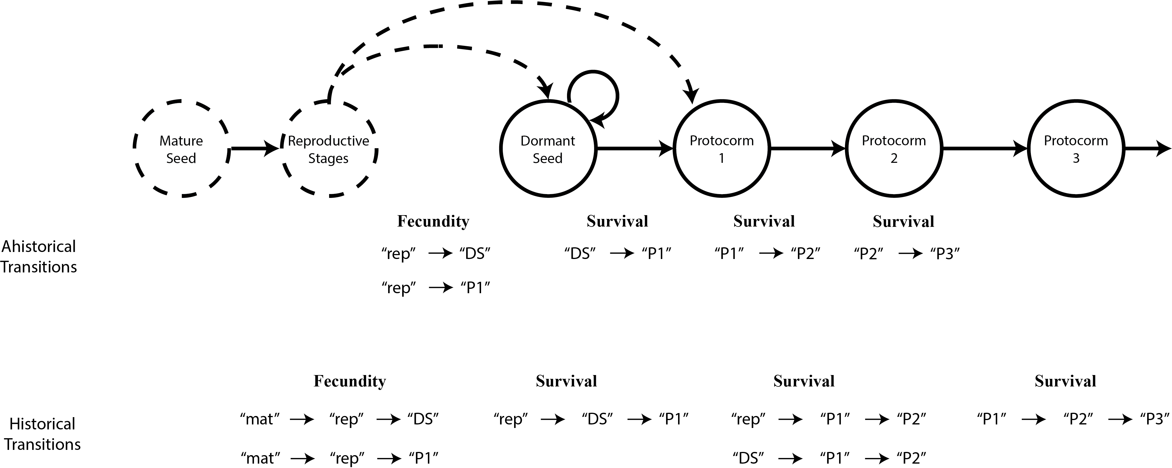
The most important thing to consider in building a supplement table, then, is that all stages must be connected to all other stages as diagrammed in the original life history model. If a single transition noted in the above paragraph is missed, then at least one stage is not properly connected to the other stages in the model, and there is likely a 0 value associated with a particular transition that should have a non-zero value. In that circumstance, users will find that their MPM or IPM likely predicts a lower growth rate, and nothing that they do will be able to change it (typically, the asymptotic growth rate will not just decline, but be completely insensitive to changes in survival or fecundity transitions).
3.7.2 An older alternative to the supplement table
Supplement tables provide all of the supplemental information that we need. However, there is an alternative means of supplying this information, and that is through the creation of a reproductive matrix and an overwrite table. The reproductive matrix is an ahistorical matrix detailing where fecundity rates are set, and at what level. Cypripedium candidum produces seeds that germinate by the following growing season (stage P1, or a first year protocorm), or that remain dormant for the next year (stage SD). In the following matrix, we detail that the fecundity of each reproductive stage needs to be split into two between each of these output stages. The actual split places 50% of the fecundity of a reproductive stage into each category of recruit, where the full fecundity is estimated by linear models that we will create. This reproductive matrix can be used in historical MPM construction, and it is assumed that stage at occasion t-1 is set to all.
rep.assumptions_fb <- matrix(0, 54, 54)
rep.assumptions_fb[1:2,31:54] <- 0.5 * seeds_per_fruit
rep.assumptions_fb
>       [,1] [,2] [,3] [,4] [,5] [,6] [,7] [,8] [,9] [,10] [,11] [,12] [,13]
>  [1,]    0    0    0    0    0    0    0    0    0     0     0     0     0
>  [2,]    0    0    0    0    0    0    0    0    0     0     0     0     0
>  [3,]    0    0    0    0    0    0    0    0    0     0     0     0     0
>  [4,]    0    0    0    0    0    0    0    0    0     0     0     0     0
>  [5,]    0    0    0    0    0    0    0    0    0     0     0     0     0
>  [6,]    0    0    0    0    0    0    0    0    0     0     0     0     0
>  [7,]    0    0    0    0    0    0    0    0    0     0     0     0     0
>  [8,]    0    0    0    0    0    0    0    0    0     0     0     0     0
>  [9,]    0    0    0    0    0    0    0    0    0     0     0     0     0
> [10,]    0    0    0    0    0    0    0    0    0     0     0     0     0
> [11,]    0    0    0    0    0    0    0    0    0     0     0     0     0
> [12,]    0    0    0    0    0    0    0    0    0     0     0     0     0
> [13,]    0    0    0    0    0    0    0    0    0     0     0     0     0
> [14,]    0    0    0    0    0    0    0    0    0     0     0     0     0
> [15,]    0    0    0    0    0    0    0    0    0     0     0     0     0
> [16,]    0    0    0    0    0    0    0    0    0     0     0     0     0
> [17,]    0    0    0    0    0    0    0    0    0     0     0     0     0
> [18,]    0    0    0    0    0    0    0    0    0     0     0     0     0
>       [,14] [,15] [,16] [,17] [,18] [,19] [,20] [,21] [,22] [,23] [,24] [,25]
>  [1,]     0     0     0     0     0     0     0     0     0     0     0     0
>  [2,]     0     0     0     0     0     0     0     0     0     0     0     0
>  [3,]     0     0     0     0     0     0     0     0     0     0     0     0
>  [4,]     0     0     0     0     0     0     0     0     0     0     0     0
>  [5,]     0     0     0     0     0     0     0     0     0     0     0     0
>  [6,]     0     0     0     0     0     0     0     0     0     0     0     0
>  [7,]     0     0     0     0     0     0     0     0     0     0     0     0
>  [8,]     0     0     0     0     0     0     0     0     0     0     0     0
>  [9,]     0     0     0     0     0     0     0     0     0     0     0     0
> [10,]     0     0     0     0     0     0     0     0     0     0     0     0
> [11,]     0     0     0     0     0     0     0     0     0     0     0     0
> [12,]     0     0     0     0     0     0     0     0     0     0     0     0
> [13,]     0     0     0     0     0     0     0     0     0     0     0     0
> [14,]     0     0     0     0     0     0     0     0     0     0     0     0
> [15,]     0     0     0     0     0     0     0     0     0     0     0     0
> [16,]     0     0     0     0     0     0     0     0     0     0     0     0
> [17,]     0     0     0     0     0     0     0     0     0     0     0     0
> [18,]     0     0     0     0     0     0     0     0     0     0     0     0
>       [,26] [,27] [,28] [,29] [,30] [,31] [,32] [,33] [,34] [,35] [,36] [,37]
>  [1,]     0     0     0     0     0  2500  2500  2500  2500  2500  2500  2500
>  [2,]     0     0     0     0     0  2500  2500  2500  2500  2500  2500  2500
>  [3,]     0     0     0     0     0     0     0     0     0     0     0     0
>  [4,]     0     0     0     0     0     0     0     0     0     0     0     0
>  [5,]     0     0     0     0     0     0     0     0     0     0     0     0
>  [6,]     0     0     0     0     0     0     0     0     0     0     0     0
>  [7,]     0     0     0     0     0     0     0     0     0     0     0     0
>  [8,]     0     0     0     0     0     0     0     0     0     0     0     0
>  [9,]     0     0     0     0     0     0     0     0     0     0     0     0
> [10,]     0     0     0     0     0     0     0     0     0     0     0     0
> [11,]     0     0     0     0     0     0     0     0     0     0     0     0
> [12,]     0     0     0     0     0     0     0     0     0     0     0     0
> [13,]     0     0     0     0     0     0     0     0     0     0     0     0
> [14,]     0     0     0     0     0     0     0     0     0     0     0     0
> [15,]     0     0     0     0     0     0     0     0     0     0     0     0
> [16,]     0     0     0     0     0     0     0     0     0     0     0     0
> [17,]     0     0     0     0     0     0     0     0     0     0     0     0
> [18,]     0     0     0     0     0     0     0     0     0     0     0     0
>       [,38] [,39] [,40] [,41] [,42] [,43] [,44] [,45] [,46] [,47] [,48] [,49]
>  [1,]  2500  2500  2500  2500  2500  2500  2500  2500  2500  2500  2500  2500
>  [2,]  2500  2500  2500  2500  2500  2500  2500  2500  2500  2500  2500  2500
>  [3,]     0     0     0     0     0     0     0     0     0     0     0     0
>  [4,]     0     0     0     0     0     0     0     0     0     0     0     0
>  [5,]     0     0     0     0     0     0     0     0     0     0     0     0
>  [6,]     0     0     0     0     0     0     0     0     0     0     0     0
>  [7,]     0     0     0     0     0     0     0     0     0     0     0     0
>  [8,]     0     0     0     0     0     0     0     0     0     0     0     0
>  [9,]     0     0     0     0     0     0     0     0     0     0     0     0
> [10,]     0     0     0     0     0     0     0     0     0     0     0     0
> [11,]     0     0     0     0     0     0     0     0     0     0     0     0
> [12,]     0     0     0     0     0     0     0     0     0     0     0     0
> [13,]     0     0     0     0     0     0     0     0     0     0     0     0
> [14,]     0     0     0     0     0     0     0     0     0     0     0     0
> [15,]     0     0     0     0     0     0     0     0     0     0     0     0
> [16,]     0     0     0     0     0     0     0     0     0     0     0     0
> [17,]     0     0     0     0     0     0     0     0     0     0     0     0
> [18,]     0     0     0     0     0     0     0     0     0     0     0     0
>       [,50] [,51] [,52] [,53] [,54]
>  [1,]  2500  2500  2500  2500  2500
>  [2,]  2500  2500  2500  2500  2500
>  [3,]     0     0     0     0     0
>  [4,]     0     0     0     0     0
>  [5,]     0     0     0     0     0
>  [6,]     0     0     0     0     0
>  [7,]     0     0     0     0     0
>  [8,]     0     0     0     0     0
>  [9,]     0     0     0     0     0
> [10,]     0     0     0     0     0
> [11,]     0     0     0     0     0
> [12,]     0     0     0     0     0
> [13,]     0     0     0     0     0
> [14,]     0     0     0     0     0
> [15,]     0     0     0     0     0
> [16,]     0     0     0     0     0
> [17,]     0     0     0     0     0
> [18,]     0     0     0     0     0
>  [ reached 'max' / getOption("max.print") -- omitted 36 rows ]
Next we will create the overwrite tables, which outline transitions that cannot be estimated from the data set and need to be set by other means. Here is an example of two overwrite tables for the Cypripedium candidum analysis. Note that they are fundamentally similar to supplement tables, but do not allow the addition of multipliers and transition types from occasion t-1 to t, they do not allow the addition of offsets, and entering them does not involve a check of entered stages against the stageframe.
cypover3_fb <- overwrite(stage3 = c("SD", "SD", "P1", "P1", "P2", "P3", "SL",
    "SL", "SL", "Dorm", "1V", "2V", "3V", "Dorm", "1V", "2V", "3V", "mat",
    "mat", "mat", "mat"),
  stage2 = c("SD", "SD", "SD", "SD", "P1", "P2", "P3", "SL", "SL", "SL", "SL",
    "SL", "SL", "SL", "SL", "SL", "SL", "Dorm", "1V", "2V", "3V"),
  stage1 = c("SD", "rep", "SD", "rep", "SD", "P1", "P2", "P3", "SL", "P3", "P3",
    "P3", "P3", "SL", "SL", "SL", "SL", "SL", "SL", "SL", "SL"),
  eststage3 = c(NA, NA, NA, NA, NA, NA, NA, NA, NA, "Dorm", "1V", "2V", "3V",
    "Dorm", "1V", "2V", "3V", "mat", "mat", "mat", "mat"),
  eststage2 = c(NA, NA, NA, NA, NA, NA, NA, NA, NA, "Dorm", "Dorm", "Dorm",
    "Dorm", "Dorm", "Dorm", "Dorm", "Dorm", "Dorm", "1V", "2V", "3V"),
  eststage1 = c(NA, NA, NA, NA, NA, NA, NA, NA, NA, "Dorm", "Dorm", "Dorm",
    "Dorm", "Dorm", "Dorm", "Dorm", "Dorm", "1V", "1V", "1V", "1V"),
  givenrate = c(0.08, 0.08, 0.1, 0.1, 0.1, 0.1, 0.1, 0.05, 0.05, NA, NA, NA, NA,
    NA, NA, NA, NA, NA, NA, NA, NA))
> This function is deprecated. Please use supplemental() instead

cypover3_fb
>    stage3 stage2 stage1 eststage3 eststage2 eststage1 givenrate convtype
> 1      SD     SD     SD      <NA>      <NA>      <NA>      0.08        1
> 2      SD     SD    rep      <NA>      <NA>      <NA>      0.08        1
> 3      P1     SD     SD      <NA>      <NA>      <NA>      0.10        1
> 4      P1     SD    rep      <NA>      <NA>      <NA>      0.10        1
> 5      P2     P1     SD      <NA>      <NA>      <NA>      0.10        1
> 6      P3     P2     P1      <NA>      <NA>      <NA>      0.10        1
> 7      SL     P3     P2      <NA>      <NA>      <NA>      0.10        1
> 8      SL     SL     P3      <NA>      <NA>      <NA>      0.05        1
> 9      SL     SL     SL      <NA>      <NA>      <NA>      0.05        1
> 10   Dorm     SL     P3      Dorm      Dorm      Dorm        NA        1
> 11     1V     SL     P3        1V      Dorm      Dorm        NA        1
> 12     2V     SL     P3        2V      Dorm      Dorm        NA        1
> 13     3V     SL     P3        3V      Dorm      Dorm        NA        1
> 14   Dorm     SL     SL      Dorm      Dorm      Dorm        NA        1
> 15     1V     SL     SL        1V      Dorm      Dorm        NA        1
> 16     2V     SL     SL        2V      Dorm      Dorm        NA        1
> 17     3V     SL     SL        3V      Dorm      Dorm        NA        1
> 18    mat   Dorm     SL       mat      Dorm        1V        NA        1
> 19    mat     1V     SL       mat        1V        1V        NA        1
> 20    mat     2V     SL       mat        2V        1V        NA        1
> 21    mat     3V     SL       mat        3V        1V        NA        1
>    convtype_t12
> 1             1
> 2             1
> 3             1
> 4             1
> 5             1
> 6             1
> 7             1
> 8             1
> 9             1
> 10            1
> 11            1
> 12            1
> 13            1
> 14            1
> 15            1
> 16            1
> 17            1
> 18            1
> 19            1
> 20            1
> 21            1

cypover2_fb <- overwrite(stage3 = c("SD", "P1", "P2", "P3", "SL", "SL", "Dorm",
    "1V", "2V", "3V"),
  stage2 = c("SD", "SD", "P1", "P2", "P3", "SL", "SL", "SL", "SL", "SL"),
  eststage3 = c(NA, NA, NA, NA, NA, NA, "Dorm", "1V", "2V", "3V"),
  eststage2 = c(NA, NA, NA, NA, NA, NA, "Dorm", "Dorm", "Dorm", "Dorm"),
  givenrate = c(0.08, 0.1, 0.1, 0.1, 0.05, 0.05, NA, NA, NA, NA),
  type = c("S", "S", "S", "S", "S", "S", "S", "S", "S"))
> This function is deprecated. Please use supplemental() instead

cypover2_fb
>    stage3 stage2 stage1 eststage3 eststage2 eststage1 givenrate convtype
> 1      SD     SD   <NA>      <NA>      <NA>      <NA>      0.08        1
> 2      P1     SD   <NA>      <NA>      <NA>      <NA>      0.10        1
> 3      P2     P1   <NA>      <NA>      <NA>      <NA>      0.10        1
> 4      P3     P2   <NA>      <NA>      <NA>      <NA>      0.10        1
> 5      SL     P3   <NA>      <NA>      <NA>      <NA>      0.05        1
> 6      SL     SL   <NA>      <NA>      <NA>      <NA>      0.05        1
> 7    Dorm     SL   <NA>      Dorm      Dorm      <NA>        NA        1
> 8      1V     SL   <NA>        1V      Dorm      <NA>        NA        1
> 9      2V     SL   <NA>        2V      Dorm      <NA>        NA        1
> 10     3V     SL   <NA>        3V      Dorm      <NA>        NA        1
>    convtype_t12
> 1             1
> 2             1
> 3             1
> 4             1
> 5             1
> 6             1
> 7             1
> 8             1
> 9             1
> 10            1
Let’s now also supply the overwrite tables and reproductive matrix for the raw MPMs.
rep_cyp_raw <- matrix(0, 11, 11)
rep_cyp_raw[1:2,7:11] <- 0.5 * seeds_per_fruit

rep_cyp_raw
>       [,1] [,2] [,3] [,4] [,5] [,6] [,7] [,8] [,9] [,10] [,11]
>  [1,]    0    0    0    0    0    0 2500 2500 2500  2500  2500
>  [2,]    0    0    0    0    0    0 2500 2500 2500  2500  2500
>  [3,]    0    0    0    0    0    0    0    0    0     0     0
>  [4,]    0    0    0    0    0    0    0    0    0     0     0
>  [5,]    0    0    0    0    0    0    0    0    0     0     0
>  [6,]    0    0    0    0    0    0    0    0    0     0     0
>  [7,]    0    0    0    0    0    0    0    0    0     0     0
>  [8,]    0    0    0    0    0    0    0    0    0     0     0
>  [9,]    0    0    0    0    0    0    0    0    0     0     0
> [10,]    0    0    0    0    0    0    0    0    0     0     0
> [11,]    0    0    0    0    0    0    0    0    0     0     0

cypover2_raw <- overwrite(stage3 = c("SD", "P1", "P2", "P3", "SL", "SL", "Dorm",
    "XSm", "Sm"),
  stage2 = c("SD", "SD", "P1", "P2", "P3", "SL", "SL", "SL", "SL"),
  eststage3 = c(NA, NA, NA, NA, NA, NA, "Dorm", "XSm", "Sm"),
  eststage2 = c(NA, NA, NA, NA, NA, NA, "XSm", "XSm", "XSm"),
  givenrate = c(0.08, 0.10, 0.10, 0.10, 0.05, 0.05, NA, NA, NA),
  type = c("S", "S", "S", "S", "S", "S", "S", "S", "S"))
> This function is deprecated. Please use supplemental() instead

cypover2_raw
>   stage3 stage2 stage1 eststage3 eststage2 eststage1 givenrate convtype
> 1     SD     SD   <NA>      <NA>      <NA>      <NA>      0.08        1
> 2     P1     SD   <NA>      <NA>      <NA>      <NA>      0.10        1
> 3     P2     P1   <NA>      <NA>      <NA>      <NA>      0.10        1
> 4     P3     P2   <NA>      <NA>      <NA>      <NA>      0.10        1
> 5     SL     P3   <NA>      <NA>      <NA>      <NA>      0.05        1
> 6     SL     SL   <NA>      <NA>      <NA>      <NA>      0.05        1
> 7   Dorm     SL   <NA>      Dorm       XSm      <NA>        NA        1
> 8    XSm     SL   <NA>       XSm       XSm      <NA>        NA        1
> 9     Sm     SL   <NA>        Sm       XSm      <NA>        NA        1
>   convtype_t12
> 1            1
> 2            1
> 3            1
> 4            1
> 5            1
> 6            1
> 7            1
> 8            1
> 9            1

cypover3_raw <- overwrite(stage3 = c("SD", "SD", "P1", "P1", "P2", "P2",
    "P3", "SL", "SL", "SL", "Dorm", "XSm", "Sm", "Dorm", "XSm", "Sm", "mat",
    "mat", "mat"),
  stage2 = c("SD", "SD", "SD", "SD", "P1", "P1", "P2", "P3", "SL", "SL", "SL",
    "SL", "SL", "SL", "SL", "SL", "Dorm", "XSm", "Sm"),
  stage1 = c("SD", "rep", "SD", "rep", "SD", "rep", "P1", "P2", "P3", "SL",
    "SL", "SL", "SL", "P3", "P3", "P3", "SL", "SL", "SL"),
  eststage3 = c(NA, NA, NA, NA, NA, NA, NA, NA, NA, NA, "Dorm", "XSm", "Sm",
    "Dorm", "XSm", "Sm", "mat", "mat", "mat"),
  eststage2 = c(NA, NA, NA, NA, NA, NA, NA, NA, NA, NA, "XSm", "XSm", "XSm",
    "XSm", "XSm", "XSm", "Dorm", "XSm", "Sm"),
  eststage1 = c(NA, NA, NA, NA, NA, NA, NA, NA, NA, NA, "XSm", "XSm", "XSm",
    "XSm", "XSm", "XSm", "XSm", "XSm", "XSm"),
  givenrate = c(0.08, 0.10, 0.10, 0.10, 0.10, 0.10, 0.10, 0.05, 0.05, 0.05, NA,
    NA, NA, NA, NA, NA, NA, NA, NA),
  type = c("S", "S", "S", "S", "S", "S", "S", "S", "S", "S", "S", "S"))
> This function is deprecated. Please use supplemental() instead

cypover3_raw
>    stage3 stage2 stage1 eststage3 eststage2 eststage1 givenrate convtype
> 1      SD     SD     SD      <NA>      <NA>      <NA>      0.08        1
> 2      SD     SD    rep      <NA>      <NA>      <NA>      0.10        1
> 3      P1     SD     SD      <NA>      <NA>      <NA>      0.10        1
> 4      P1     SD    rep      <NA>      <NA>      <NA>      0.10        1
> 5      P2     P1     SD      <NA>      <NA>      <NA>      0.10        1
> 6      P2     P1    rep      <NA>      <NA>      <NA>      0.10        1
> 7      P3     P2     P1      <NA>      <NA>      <NA>      0.10        1
> 8      SL     P3     P2      <NA>      <NA>      <NA>      0.05        1
> 9      SL     SL     P3      <NA>      <NA>      <NA>      0.05        1
> 10     SL     SL     SL      <NA>      <NA>      <NA>      0.05        1
> 11   Dorm     SL     SL      Dorm       XSm       XSm        NA        1
> 12    XSm     SL     SL       XSm       XSm       XSm        NA        1
> 13     Sm     SL     SL        Sm       XSm       XSm        NA        1
> 14   Dorm     SL     P3      Dorm       XSm       XSm        NA        1
> 15    XSm     SL     P3       XSm       XSm       XSm        NA        1
> 16     Sm     SL     P3        Sm       XSm       XSm        NA        1
> 17    mat   Dorm     SL       mat      Dorm       XSm        NA        1
> 18    mat    XSm     SL       mat       XSm       XSm        NA        1
> 19    mat     Sm     SL       mat        Sm       XSm        NA        1
>    convtype_t12
> 1             1
> 2             1
> 3             1
> 4             1
> 5             1
> 6             1
> 7             1
> 8             1
> 9             1
> 10            1
> 11            1
> 12            1
> 13            1
> 14            1
> 15            1
> 16            1
> 17            1
> 18            1
> 19            1
The overwrite() approach is much less powerful than the supplement table approach, particularly because it lacks the ability to handle multipliers and offsets, it lacks some shorthand stage abbreviations, and it lacks inconsistency checks. The supplemental() approach can also provide supplement tables for all kinds of MPs / IPMs developed in lefko3, including age-by-stage and even Leslie MPMs, and is actively maintained while overwrite() is now deprecated. So, we encourage the use of supplemental() rather than overwrite().
3.8 Handling complex life histories
Situations may occur in which the life history of the organism includes two sets of stages with transitions only occurring in one direction between them. For example, let’s consider the following life history model (figure 3.4).
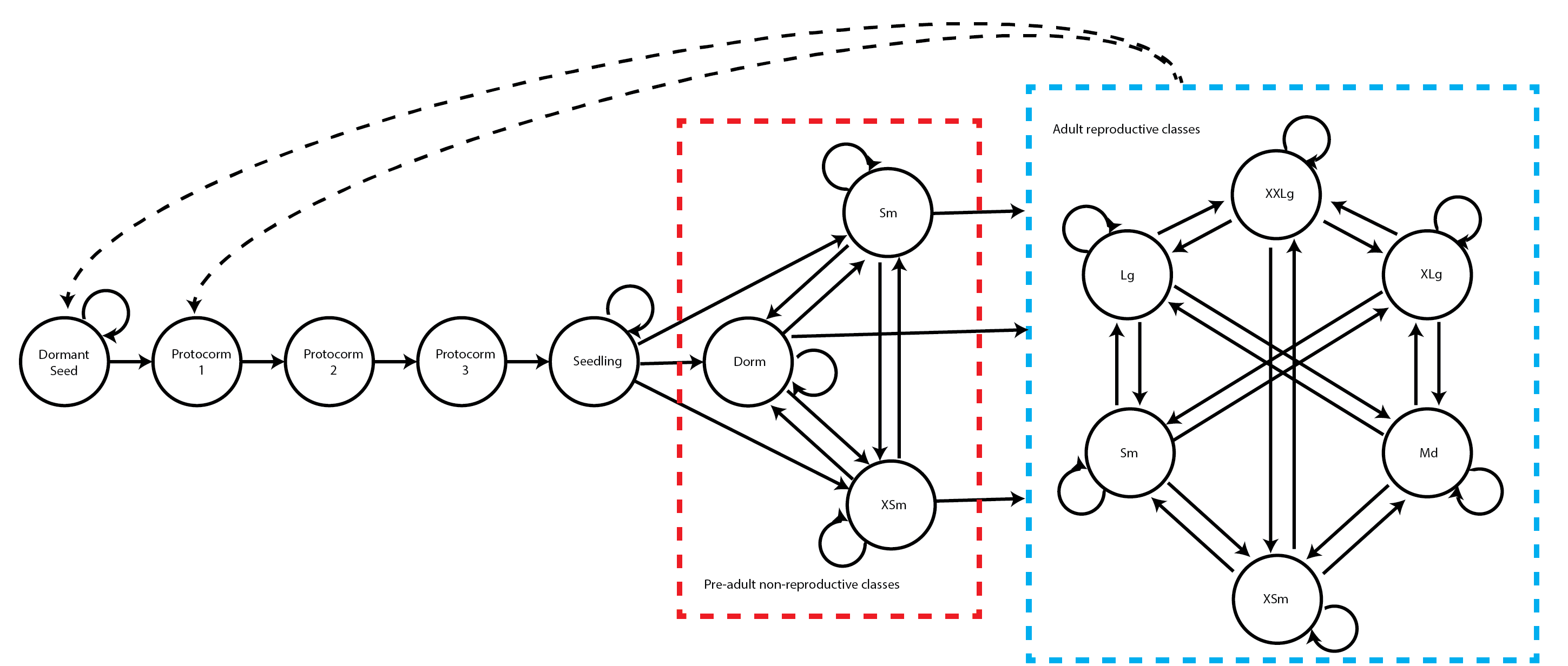
Raw MPMs have no problem with this situation, provided that each stage has its own, unique set of characteristics. However, function-based MPM (including IPM) creation functions will have a default tendency to estimate survival transitions from the adult reproductive stages (in blue box) back to the pre-adult non-reproductive stages (in red box), in addition to the transitions shown in the figure. We can deal with this problem using stage grouping.
First, we will create a new stageframe that encapsulates all of the stages above. Note that the primary addition that we will make to the sf_create() input is the group option.
sizevector <- c(0, 0, 0, 0, 0, 0, 1, 3, 1, 3, 6, 11, 20, 31)
stagevector <- c("SD", "P1", "P2", "P3", "SL", "preDorm", "preXSm", "preSm",
  "XSm", "Sm", "Md", "Lg", "XLg", "XXLg")
repvector <- c(0, 0, 0, 0, 0, 0, 0, 0, 1, 1, 1, 1, 1, 1)
obsvector <- c(0, 0, 0, 0, 0, 0, 1, 1, 1, 1, 1, 1, 1, 1)
matvector <- c(0, 0, 0, 0, 0, 0, 0, 0, 1, 1, 1, 1, 1, 1)
immvector <- c(0, 1, 1, 1, 1, 1, 1, 1, 0, 0, 0, 0, 0, 0)
propvector <- c(1, 0, 0, 0, 0, 0, 0, 0, 0, 0, 0, 0, 0, 0)
indataset <- c(0, 0, 0, 0, 0, 1, 1, 1, 1, 1, 1, 1, 1, 1)
binvec <- c(0, 0, 0, 0, 0, 0.5, 0.5, 1.5, 0.5, 1.5, 1.5, 3.5, 5.5, 5.5)
group <- c(0, 0, 0, 0, 0, 1, 1, 1, 2, 2, 2, 2, 2, 2)

comments <- c("Dormant seed", "1st yr protocorm", "2nd yr protocorm",
  "3rd yr protocorm", "Seedling", "Dormant pre-adult",
  "Extra small pre-adult (1 shoot)", "Small pre-adult (2-4 shoots)",
  "Extra small adult (1 shoot)", "Small adult (2-4 shoots)",
  "Medium adult (5-7 shoots)", "Large adult (8-14 shoots)",
  "Extra large adult (20 shoots)", "Extra extra large adult (>24.5 shoots")

cypframe_alt <- sf_create(sizes = sizevector, stagenames = stagevector,
  repstatus = repvector, obsstatus = obsvector, matstatus = matvector,
  propstatus = propvector, immstatus = immvector, indataset = indataset,
  binhalfwidth = binvec, group = group, comments = comments)

cypframe_alt
>      stage size size_b size_c min_age max_age repstatus obsstatus propstatus
> 1       SD    0     NA     NA      NA      NA         0         0          1
> 2       P1    0     NA     NA      NA      NA         0         0          0
> 3       P2    0     NA     NA      NA      NA         0         0          0
> 4       P3    0     NA     NA      NA      NA         0         0          0
> 5       SL    0     NA     NA      NA      NA         0         0          0
> 6  preDorm    0     NA     NA      NA      NA         0         0          0
> 7   preXSm    1     NA     NA      NA      NA         0         1          0
> 8    preSm    3     NA     NA      NA      NA         0         1          0
> 9      XSm    1     NA     NA      NA      NA         1         1          0
> 10      Sm    3     NA     NA      NA      NA         1         1          0
> 11      Md    6     NA     NA      NA      NA         1         1          0
> 12      Lg   11     NA     NA      NA      NA         1         1          0
> 13     XLg   20     NA     NA      NA      NA         1         1          0
> 14    XXLg   31     NA     NA      NA      NA         1         1          0
>    immstatus matstatus indataset binhalfwidth_raw sizebin_min sizebin_max
> 1          0         0         0              0.0         0.0         0.0
> 2          1         0         0              0.0         0.0         0.0
> 3          1         0         0              0.0         0.0         0.0
> 4          1         0         0              0.0         0.0         0.0
> 5          1         0         0              0.0         0.0         0.0
> 6          1         0         1              0.5        -0.5         0.5
> 7          1         0         1              0.5         0.5         1.5
> 8          1         0         1              1.5         1.5         4.5
> 9          0         1         1              0.5         0.5         1.5
> 10         0         1         1              1.5         1.5         4.5
> 11         0         1         1              1.5         4.5         7.5
> 12         0         1         1              3.5         7.5        14.5
> 13         0         1         1              5.5        14.5        25.5
> 14         0         1         1              5.5        25.5        36.5
>    sizebin_center sizebin_width binhalfwidthb_raw sizebinb_min sizebinb_max
> 1               0             0                NA           NA           NA
> 2               0             0                NA           NA           NA
> 3               0             0                NA           NA           NA
> 4               0             0                NA           NA           NA
> 5               0             0                NA           NA           NA
> 6               0             1                NA           NA           NA
> 7               1             1                NA           NA           NA
> 8               3             3                NA           NA           NA
> 9               1             1                NA           NA           NA
> 10              3             3                NA           NA           NA
> 11              6             3                NA           NA           NA
> 12             11             7                NA           NA           NA
> 13             20            11                NA           NA           NA
> 14             31            11                NA           NA           NA
>    sizebinb_center sizebinb_width binhalfwidthc_raw sizebinc_min sizebinc_max
> 1               NA             NA                NA           NA           NA
> 2               NA             NA                NA           NA           NA
> 3               NA             NA                NA           NA           NA
> 4               NA             NA                NA           NA           NA
> 5               NA             NA                NA           NA           NA
> 6               NA             NA                NA           NA           NA
> 7               NA             NA                NA           NA           NA
> 8               NA             NA                NA           NA           NA
> 9               NA             NA                NA           NA           NA
> 10              NA             NA                NA           NA           NA
> 11              NA             NA                NA           NA           NA
> 12              NA             NA                NA           NA           NA
> 13              NA             NA                NA           NA           NA
> 14              NA             NA                NA           NA           NA
>    sizebinc_center sizebinc_width group                              comments
> 1               NA             NA     0                          Dormant seed
> 2               NA             NA     0                      1st yr protocorm
> 3               NA             NA     0                      2nd yr protocorm
> 4               NA             NA     0                      3rd yr protocorm
> 5               NA             NA     0                              Seedling
> 6               NA             NA     1                     Dormant pre-adult
> 7               NA             NA     1       Extra small pre-adult (1 shoot)
> 8               NA             NA     1          Small pre-adult (2-4 shoots)
> 9               NA             NA     2           Extra small adult (1 shoot)
> 10              NA             NA     2              Small adult (2-4 shoots)
> 11              NA             NA     2             Medium adult (5-7 shoots)
> 12              NA             NA     2             Large adult (8-14 shoots)
> 13              NA             NA     2         Extra large adult (20 shoots)
> 14              NA             NA     2 Extra extra large adult (>24.5 shoots
Now that we have our stageframe, the only thing we need to do is to specify that survival-transitions from group 2 stages to group 1 stages are equal to 0. We can do this with the supplemental() function. Here, we will set these transitions, and also set the fecundity multipliers as before.
cypsupp2_alt <- supplemental(stage3 = c("group1", "SD", "P1"),
  stage2 = c("group2", "rep", "rep"), eststage3 = c(NA, NA, NA),
  eststage2 = c(NA, NA, NA), givenrate = c(0, NA, NA),
  multiplier = c(NA, (0.5 * seeds_per_fruit), (0.5 * seeds_per_fruit)),
  type =c(1, 3, 3), stageframe = cypframe_alt, historical = FALSE)
> Warning: NA values in argument multiplier will be treated as 1 values.
> Warning: NA values in argument multiplier will be treated as 1 values.
> Warning: NA values in argument multiplier will be treated as 1 values.

cypsupp2_alt
>   stage3 stage2 stage1 age2 eststage3 eststage2 eststage1 estage2 givenrate
> 1 group1 group2   <NA>   NA      <NA>      <NA>      <NA>      NA         0
> 2     SD    rep   <NA>   NA      <NA>      <NA>      <NA>      NA        NA
> 3     P1    rep   <NA>   NA      <NA>      <NA>      <NA>      NA        NA
>   offset multiplier convtype convtype_t12
> 1     NA          1        1            1
> 2     NA       2500        3            1
> 3     NA       2500        3            1
This supplement table can now be input into a matrix estimator function to tell that function that these transitions must be 0. We will see how to do this with different styles of MPM in the next four chapters.
3.9 Bootstrapping demographic data
Users may at times wish to bootstrap their demographic data. Applications might include testing the impacts of demographic stochasticity, or estimating standard errors on parameters such as the asymptotic population growth rate. Function bootstrap3() can help with this. Here, we see an example in which we bootstrap one of our hfv format datasets to produce three replicates.
set.seed(42)
cypboot <- bootstrap3(cypraw_v1, reps = 3)

summary_hfv(cypboot)
>
> This hfvlist object contains 3 hfvdata demographic data frames.
> Each data frame contains an average of 306.333 rows, 57 variables, 1 population,
> 3 patches, 44.667 individuals, and 5 time steps.
>
> Across all data frames, there are 1 unique population, 3 unique patches, 72 unique individuals, and 5 unique time steps.
The result is a list of class hfvlist, which is composed of elements each of which is a replicated dataset of class hfvdata. Function bootstrap3() resamples by individual by default, and will also keep the numbers of total individuals within each resampled population and patch equivalent to the original numbers of individuals. The result will typically be a lower number of unique individuals in each part and population, since some unique individuals will be repeatedly sampled while others will not be chosen at all. If we wish, we can change this, for example by setting by_indiv = FALSE.
set.seed(42)
cypboot_alt <- bootstrap3(cypraw_v1, reps = 3, by_indiv = FALSE)

summary_hfv(cypboot_alt)
>
> This hfvlist object contains 3 hfvdata demographic data frames.
> Each data frame contains an average of 320 rows, 57 variables, 1 population,
> 3 patches, 70.333 individuals, and 5 time steps.
>
> Across all data frames, there are 1 unique population, 3 unique patches, 74 unique individuals, and 5 unique time steps.
To utilize individual resampled datasets, just refer to them by using the object name and the associated list element. For example, to see a summary of the 2nd replicate of cypboot_alt, we can type the following.
summary_hfv(cypboot_alt[[2]], full = TRUE)
>
> This hfv dataset contains 320 rows, 57 variables, 1 population,
> 3 patches, 69 individuals, and 5 time steps.
>      rowid          popid           patchid    individ         year2
>  Min.   : 1.00   Length:320         A: 93   Min.   : 164   Min.   :2004
>  1st Qu.:21.00   Class :character   B:154   1st Qu.: 391   1st Qu.:2005
>  Median :37.00   Mode  :character   C: 73   Median : 452   Median :2006
>  Mean   :38.12                              Mean   : 649   Mean   :2006
>  3rd Qu.:56.00                              3rd Qu.: 476   3rd Qu.:2007
>  Max.   :77.00                              Max.   :1560   Max.   :2008
>    firstseen       lastseen        obsage       obslifespan        sizea1
>  Min.   :2004   Min.   :2004   Min.   :5.000   Min.   :0.000   Min.   :0
>  1st Qu.:2004   1st Qu.:2009   1st Qu.:6.000   1st Qu.:5.000   1st Qu.:0
>  Median :2004   Median :2009   Median :7.000   Median :5.000   Median :0
>  Mean   :2004   Mean   :2009   Mean   :6.819   Mean   :4.638   Mean   :0
>  3rd Qu.:2004   3rd Qu.:2009   3rd Qu.:8.000   3rd Qu.:5.000   3rd Qu.:0
>  Max.   :2008   Max.   :2009   Max.   :9.000   Max.   :5.000   Max.   :0
>      sizeb1            sizec1         size1added        repstra1
>  Min.   : 0.0000   Min.   : 0.000   Min.   : 0.000   Min.   : 0.0000
>  1st Qu.: 0.0000   1st Qu.: 0.000   1st Qu.: 0.000   1st Qu.: 0.0000
>  Median : 0.0000   Median : 1.000   Median : 1.500   Median : 0.0000
>  Mean   : 0.8063   Mean   : 1.991   Mean   : 2.797   Mean   : 0.8063
>  3rd Qu.: 1.0000   3rd Qu.: 3.000   3rd Qu.: 4.000   3rd Qu.: 1.0000
>  Max.   :18.0000   Max.   :12.000   Max.   :21.000   Max.   :18.0000
>     repstrb1  repstr1added         feca1          fec1added
>  Min.   :0   Min.   : 0.0000   Min.   :0.0000   Min.   :0.0000
>  1st Qu.:0   1st Qu.: 0.0000   1st Qu.:0.0000   1st Qu.:0.0000
>  Median :0   Median : 0.0000   Median :0.0000   Median :0.0000
>  Mean   :0   Mean   : 0.8063   Mean   :0.2719   Mean   :0.2719
>  3rd Qu.:0   3rd Qu.: 1.0000   3rd Qu.:0.0000   3rd Qu.:0.0000
>  Max.   :0   Max.   :18.0000   Max.   :7.0000   Max.   :7.0000
>    obsstatus1       repstatus1       fecstatus1       matstatus1
>  Min.   :0.0000   Min.   :0.0000   Min.   :0.0000   Min.   :0.0000
>  1st Qu.:0.0000   1st Qu.:0.0000   1st Qu.:0.0000   1st Qu.:1.0000
>  Median :1.0000   Median :0.0000   Median :0.0000   Median :1.0000
>  Mean   :0.7469   Mean   :0.2875   Mean   :0.1469   Mean   :0.7688
>  3rd Qu.:1.0000   3rd Qu.:1.0000   3rd Qu.:0.0000   3rd Qu.:1.0000
>  Max.   :1.0000   Max.   :1.0000   Max.   :1.0000   Max.   :1.0000
>      alive1          stage1           stage1index         sizea2
>  Min.   :0.0000   Length:320         Min.   : 0.000   Min.   :0.0000
>  1st Qu.:1.0000   Class :character   1st Qu.: 6.000   1st Qu.:0.0000
>  Median :1.0000   Mode  :character   Median : 7.500   Median :0.0000
>  Mean   :0.7688                      Mean   : 6.172   Mean   :0.0125
>  3rd Qu.:1.0000                      3rd Qu.: 8.000   3rd Qu.:0.0000
>  Max.   :1.0000                      Max.   :11.000   Max.   :1.0000
>      sizeb2           sizec2         size2added        repstra2
>  Min.   : 0.000   Min.   : 0.000   Min.   : 0.000   Min.   : 0.000
>  1st Qu.: 0.000   1st Qu.: 1.000   1st Qu.: 1.000   1st Qu.: 0.000
>  Median : 0.000   Median : 1.000   Median : 2.000   Median : 0.000
>  Mean   : 1.041   Mean   : 2.472   Mean   : 3.525   Mean   : 1.041
>  3rd Qu.: 1.000   3rd Qu.: 4.000   3rd Qu.: 4.000   3rd Qu.: 1.000
>  Max.   :18.000   Max.   :13.000   Max.   :24.000   Max.   :18.000
>     repstrb2       repstr2added        feca2       fec2added     obsstatus2
>  Min.   :0.0000   Min.   : 0.000   Min.   :0.0   Min.   :0.0   Min.   :0.00
>  1st Qu.:0.0000   1st Qu.: 0.000   1st Qu.:0.0   1st Qu.:0.0   1st Qu.:1.00
>  Median :0.0000   Median : 0.000   Median :0.0   Median :0.0   Median :1.00
>  Mean   :0.0125   Mean   : 1.053   Mean   :0.3   Mean   :0.3   Mean   :0.95
>  3rd Qu.:0.0000   3rd Qu.: 1.000   3rd Qu.:0.0   3rd Qu.:0.0   3rd Qu.:1.00
>  Max.   :1.0000   Max.   :18.000   Max.   :7.0   Max.   :7.0   Max.   :1.00
>    repstatus2       fecstatus2       matstatus2     alive2     stage2
>  Min.   :0.0000   Min.   :0.0000   Min.   :1    Min.   :1   Length:320
>  1st Qu.:0.0000   1st Qu.:0.0000   1st Qu.:1    1st Qu.:1   Class :character
>  Median :0.0000   Median :0.0000   Median :1    Median :1   Mode  :character
>  Mean   :0.3594   Mean   :0.1437   Mean   :1    Mean   :1
>  3rd Qu.:1.0000   3rd Qu.:0.0000   3rd Qu.:1    3rd Qu.:1
>  Max.   :1.0000   Max.   :1.0000   Max.   :1    Max.   :1
>   stage2index         sizea3            sizeb3           sizec3
>  Min.   : 6.000   Min.   :0.00000   Min.   : 0.000   Min.   : 0.000
>  1st Qu.: 7.000   1st Qu.:0.00000   1st Qu.: 0.000   1st Qu.: 1.000
>  Median : 8.000   Median :0.00000   Median : 0.000   Median : 1.000
>  Mean   : 7.912   Mean   :0.00625   Mean   : 1.322   Mean   : 2.169
>  3rd Qu.: 8.000   3rd Qu.:0.00000   3rd Qu.: 1.000   3rd Qu.: 3.000
>  Max.   :11.000   Max.   :1.00000   Max.   :18.000   Max.   :13.000
>    size3added        repstra3         repstrb3        repstr3added
>  Min.   : 0.000   Min.   : 0.000   Min.   :0.00000   Min.   : 0.000
>  1st Qu.: 1.000   1st Qu.: 0.000   1st Qu.:0.00000   1st Qu.: 0.000
>  Median : 2.000   Median : 0.000   Median :0.00000   Median : 0.000
>  Mean   : 3.497   Mean   : 1.322   Mean   :0.00625   Mean   : 1.328
>  3rd Qu.: 4.000   3rd Qu.: 1.000   3rd Qu.:0.00000   3rd Qu.: 1.000
>  Max.   :24.000   Max.   :18.000   Max.   :1.00000   Max.   :18.000
>      feca3          fec3added        obsstatus3       repstatus3
>  Min.   :0.0000   Min.   :0.0000   Min.   :0.0000   Min.   :0.0000
>  1st Qu.:0.0000   1st Qu.:0.0000   1st Qu.:1.0000   1st Qu.:0.0000
>  Median :0.0000   Median :0.0000   Median :1.0000   Median :0.0000
>  Mean   :0.6125   Mean   :0.6125   Mean   :0.9187   Mean   :0.4313
>  3rd Qu.:0.0000   3rd Qu.:0.0000   3rd Qu.:1.0000   3rd Qu.:1.0000
>  Max.   :8.0000   Max.   :8.0000   Max.   :1.0000   Max.   :1.0000
>    fecstatus3       matstatus3     alive3          stage3
>  Min.   :0.0000   Min.   :1    Min.   :0.0000   Length:320
>  1st Qu.:0.0000   1st Qu.:1    1st Qu.:1.0000   Class :character
>  Median :0.0000   Median :1    Median :1.0000   Mode  :character
>  Mean   :0.2313   Mean   :1    Mean   :0.9531
>  3rd Qu.:0.0000   3rd Qu.:1    3rd Qu.:1.0000
>  Max.   :1.0000   Max.   :1    Max.   :1.0000
>   stage3index
>  Min.   : 0.000
>  1st Qu.: 7.000
>  Median : 8.000
>  Mean   : 7.616
>  3rd Qu.: 8.000
>  Max.   :11.000
Function bootstrap3() includes a number of customizable arguments that will make it very useful. We will see it again in later chapters, as we estimate key parameters with bootstrapped approaches.
3.10 Points to remember
- Functions
verticalize3()andhistoricalize3()can be used to take horizontally or vertically arranged demographic datasets and standardize them into the appropriate format for MPM creation and analysis, called hfv format. - Function
summary_hfv()provides summaries of hfv datasets, including the overall dimensions, the numbers of individuals, and other important characteristics. - Function
actualstage3()provides a means of exploring standardized hfv datasets, showing the actual frequencies and proportions of each stage, age, age-stage, or historical stage-pair alive in each year. - Function
supplemental()provides the means to incorporate given transition values obtained from external studies, set transitions to proxy values to be estimated bylefko3, incorporate multipliers and offsets on survival transitions and fecundity estimates, and set proxy survival transitions. - Great care must be taken to include every missing transition within the supplement table. Otherwise, models will predict dying populations, and asymptotic analyses will be invariant to changes in survival and fecundity terms.
- Stage groups can be used to add directionality and other complex relationships between groups of life history stages.
- Demographic data can be bootstrapped with the
bootstrap3()function. This function can resample data by population, patch, and individual, with arguments to customize each ressampling.