Chapter 9 Population Projection II: Deterministic Analysis
For a moment, nothing happened. Then, after a second or so, nothing continued to happen.
Note: The example code in this chapter relies on code executed in previous chapters. This code is available in a ready-to-run block in Appendix II (19.0.3).
Deterministic analysis refers to matrix projection conducted under the assumption that a single matrix encompasses all of the important demographic variation in a population. This single matrix is projected forward to a limit of infinity, and the asymptotic properties of the projection are assessed. Projecting forward by the same matrix means that instead of going one time step forward, where \(\mathbf{n_{t+1}}=\mathbf{An_t}\), we find ourselves analyzing the result of the following equation.
\[\begin{equation} \mathbf{n_t} = \mathbf{A^tn_0}, _{t \rightarrow \infty} \tag{9.1} \end{equation}\]
The asymptotic properties of this projection conform to the results of eigenanalysis, where after some time we see the right eigenvector associated with the dominant eigenvalue yielding the equilibrial stage structure \(\mathbf{w}\), and the left eigenvector associated with the dominant eigenvalue yielding the reproductive value vector \(\mathbf{v}\). The dominant eigenvalue is \(\lambda\), and is equal to the asymptotic population growth rate. We also see the following conditions.
\[\begin{equation} \mathbf{Aw} = \lambda \mathbf{w} \tag{9.2} \end{equation}\]
\[\begin{equation} \mathbf{v^*A} = \lambda \mathbf{v^*} \tag{9.3} \end{equation}\]
Here, \(\mathbf{v^*}\) is the complex conjugate of the left eigenvector and \(\mathbf{w}\) is the right eigenvector associated with \(\lambda\) (Caswell 2001). Once we have the projected population growth rate \(\lambda\), the stable stage vector, and the reproductive value vector, we can use these terms to derive further values, such as the sensitivity or elasticity of \(\lambda\) to changes in matrix elements.
Package lefko3 includes a number of functions to aid analysis once matrices are created. These may be of greater utility in some circumstances than established R functions such as eigen(), because our functions are made to handle even extremely large, sparse matrices and can handle many kinds of unusual situations that might arise in analysis. Currently, we include functions to estimate element-wise arithmetic mean matrices, population growth rate, stable stage structure, reproductive value, sensitivity and elasticity, and one-way fixed life table response experiments (LTRE). We also include two basic projection functions that show the expected numbers of individuals in each stage forward in time under deterministic, cyclical, and stochastic conditions, with or without density dependence.
In this chapter, we will utilize the raw MPMs developed in chapter 4 to illustrate some of the deterministic analyses that we can perform. Particularly, we will use the lefkoMat objects named cypmatrix2r, cypmatrix2rp, cypmatrix3r, and cypmatrix3rp. However, the function-based MPMs, IPMs, and age-by-stage MPMs that we have created can also be used in all cases.
Let’s start off by taking a look at summaries of these four objects.
summary(cypmatrix2r)
>
> This ahistorical lefkoMat object contains 5 matrices.
>
> Each matrix is square with 11 rows and columns, and a total of 121 elements.
> A total of 120 survival transitions were estimated, with 24 per matrix.
> A total of 40 fecundity transitions were estimated, with 8 per matrix.
> This lefkoMat object covers 1 population, 1 patch, and 5 time steps.
>
> The dataset contains a total of 74 unique individuals and 320 unique transitions.
>
> Survival probability sum check (each matrix represented by column in order):
>          [,1]  [,2]  [,3]  [,4]  [,5]
> Min.    0.000 0.050 0.050 0.000 0.050
> 1st Qu. 0.100 0.140 0.140 0.100 0.140
> Median  0.689 0.870 0.864 0.610 0.882
> Mean    0.552 0.629 0.629 0.528 0.627
> 3rd Qu. 1.000 1.000 1.000 0.960 1.000
> Max.    1.000 1.000 1.000 1.000 1.000
>
>
> Stages without connections leading to the rest of the life cycle found in matrices: 1 4
summary(cypmatrix2rp)
>
> This ahistorical lefkoMat object contains 15 matrices.
>
> Each matrix is square with 11 rows and columns, and a total of 121 elements.
> A total of 266 survival transitions were estimated, with 17.733 per matrix.
> A total of 70 fecundity transitions were estimated, with 4.667 per matrix.
> This lefkoMat object covers 1 population, 3 patches, and 5 time steps.
>
> The dataset contains a total of 74 unique individuals and 320 unique transitions.
>
> Survival probability sum check (each matrix represented by column in order):
>          [,1]  [,2]  [,3]  [,4]  [,5]  [,6]  [,7]  [,8]  [,9] [,10] [,11] [,12]
> Min.    0.000 0.000 0.000 0.000 0.000 0.000 0.050 0.050 0.000 0.050 0.000 0.000
> 1st Qu. 0.075 0.025 0.075 0.025 0.075 0.075 0.140 0.140 0.100 0.140 0.100 0.100
> Median  0.180 0.100 0.180 0.100 0.180 0.180 0.909 0.778 0.686 0.857 0.750 0.575
> Mean    0.457 0.361 0.471 0.328 0.417 0.464 0.631 0.611 0.530 0.631 0.562 0.523
> 3rd Qu. 0.955 0.769 1.000 0.592 0.781 1.000 1.000 1.000 0.955 1.000 1.000 1.000
> Max.    1.000 1.000 1.000 1.000 1.000 1.000 1.000 1.000 1.000 1.000 1.000 1.000
>         [,13] [,14] [,15]
> Min.    0.000 0.000 0.000
> 1st Qu. 0.075 0.075 0.100
> Median  0.180 0.180 0.750
> Mean    0.432 0.450 0.562
> 3rd Qu. 0.875 1.000 1.000
> Max.    1.000 1.000 1.000
>
>
> Stages without connections leading to the rest of the life cycle found in matrices: 1 2 3 4 5 6 9 11 12 13 14 15
summary(cypmatrix3r)
>
> This historical lefkoMat object contains 4 matrices.
>
> Each matrix is square with 121 rows and columns, and a total of 14641 elements.
> A total of 242 survival transitions were estimated, with 60.5 per matrix.
> A total of 54 fecundity transitions were estimated, with 13.5 per matrix.
> This lefkoMat object covers 1 population, 1 patch, and 4 time steps.
>
> The dataset contains a total of 74 unique individuals and 320 unique transitions.
>
> Survival probability sum check (each matrix represented by column in order):
>          [,1]  [,2]  [,3]  [,4]
> Min.    0.000 0.000 0.000 0.000
> 1st Qu. 0.000 0.000 0.000 0.000
> Median  0.000 0.000 0.000 0.000
> Mean    0.173 0.179 0.166 0.198
> 3rd Qu. 0.100 0.100 0.100 0.100
> Max.    1.000 1.000 1.000 1.000
>
>
> Stage-pairs without connections leading to the rest of the life cycle found in matrices: 1 2 3 4
summary(cypmatrix3rp)
>
> This historical lefkoMat object contains 12 matrices.
>
> Each matrix is square with 121 rows and columns, and a total of 14641 elements.
> A total of 516 survival transitions were estimated, with 43 per matrix.
> A total of 70 fecundity transitions were estimated, with 5.833 per matrix.
> This lefkoMat object covers 1 population, 3 patches, and 4 time steps.
>
> The dataset contains a total of 74 unique individuals and 320 unique transitions.
>
> Survival probability sum check (each matrix represented by column in order):
>          [,1]   [,2]   [,3]  [,4]  [,5]  [,6] [,7]  [,8]  [,9]  [,10] [,11]
> Min.    0.000 0.0000 0.0000 0.000 0.000 0.000 0.00 0.000 0.000 0.0000 0.000
> 1st Qu. 0.000 0.0000 0.0000 0.000 0.000 0.000 0.00 0.000 0.000 0.0000 0.000
> Median  0.000 0.0000 0.0000 0.000 0.000 0.000 0.00 0.000 0.000 0.0000 0.000
> Mean    0.107 0.0945 0.0851 0.101 0.158 0.158 0.14 0.169 0.119 0.0851 0.119
> 3rd Qu. 0.000 0.0000 0.0000 0.000 0.100 0.100 0.05 0.100 0.000 0.0000 0.000
> Max.    1.000 1.0000 1.0000 1.000 1.000 1.000 1.00 1.000 1.000 1.0000 1.000
>         [,12]
> Min.    0.000
> 1st Qu. 0.000
> Median  0.000
> Mean    0.144
> 3rd Qu. 0.000
> Max.    1.000
>
>
> Stage-pairs without connections leading to the rest of the life cycle found in matrices: 1 2 3 4 5 6 7 8 9 10 11 12
We see that these four MPMs cover three patches of one population, and that cypmatrix2r and cypmatrix3r do not distinguish the patches while cypmatrix2rp and cypmatrix3rp do. Objects cypmatrix2r and cypmatrix2rp are ahistorical, while cypmatrix3r and cypmatrix3rp are historical. Because these are raw MPMs and there are six total monitoring occasions covered, we see five matrices estimated in the ahistorical population-level set and four matrices estimated in the historical population-level set. The patch-level MPMs create five and four matrices per patch for the ahistorical and historical cases, respectively. There are 11 life history stages, which we see below.
cypmatrix2r$ahstages
>    stage_id stage original_size original_size_b original_size_c min_age max_age
> 1         1    SD           0.0              NA              NA       0      NA
> 2         2    P1           0.0              NA              NA       0      NA
> 3         3    P2           0.0              NA              NA       0      NA
> 4         4    P3           0.0              NA              NA       0      NA
> 5         5    SL           0.0              NA              NA       0      NA
> 6         6  Dorm           0.0              NA              NA       0      NA
> 7         7   XSm           1.0              NA              NA       0      NA
> 8         8    Sm           3.0              NA              NA       0      NA
> 9         9    Md           6.0              NA              NA       0      NA
> 10       10    Lg          11.0              NA              NA       0      NA
> 11       11   XLg          19.5              NA              NA       0      NA
>    repstatus obsstatus propstatus immstatus matstatus entrystage indataset
> 1          0         0          1         0         0          1         0
> 2          0         0          0         1         0          1         0
> 3          0         0          0         1         0          0         0
> 4          0         0          0         1         0          0         0
> 5          0         0          0         1         0          0         0
> 6          0         0          0         0         1          0         1
> 7          1         1          0         0         1          0         1
> 8          1         1          0         0         1          0         1
> 9          1         1          0         0         1          0         1
> 10         1         1          0         0         1          0         1
> 11         1         1          0         0         1          0         1
>    binhalfwidth_raw sizebin_min sizebin_max sizebin_center sizebin_width
> 1               0.0         0.0         0.0            0.0             0
> 2               0.0         0.0         0.0            0.0             0
> 3               0.0         0.0         0.0            0.0             0
> 4               0.0         0.0         0.0            0.0             0
> 5               0.0         0.0         0.0            0.0             0
> 6               0.5        -0.5         0.5            0.0             1
> 7               0.5         0.5         1.5            1.0             1
> 8               1.5         1.5         4.5            3.0             3
> 9               1.5         4.5         7.5            6.0             3
> 10              3.5         7.5        14.5           11.0             7
> 11              5.0        14.5        24.5           19.5            10
>    binhalfwidthb_raw sizebinb_min sizebinb_max sizebinb_center sizebinb_width
> 1                 NA           NA           NA              NA             NA
> 2                 NA           NA           NA              NA             NA
> 3                 NA           NA           NA              NA             NA
> 4                 NA           NA           NA              NA             NA
> 5                 NA           NA           NA              NA             NA
> 6                 NA           NA           NA              NA             NA
> 7                 NA           NA           NA              NA             NA
> 8                 NA           NA           NA              NA             NA
> 9                 NA           NA           NA              NA             NA
> 10                NA           NA           NA              NA             NA
> 11                NA           NA           NA              NA             NA
>    binhalfwidthc_raw sizebinc_min sizebinc_max sizebinc_center sizebinc_width
> 1                 NA           NA           NA              NA             NA
> 2                 NA           NA           NA              NA             NA
> 3                 NA           NA           NA              NA             NA
> 4                 NA           NA           NA              NA             NA
> 5                 NA           NA           NA              NA             NA
> 6                 NA           NA           NA              NA             NA
> 7                 NA           NA           NA              NA             NA
> 8                 NA           NA           NA              NA             NA
> 9                 NA           NA           NA              NA             NA
> 10                NA           NA           NA              NA             NA
> 11                NA           NA           NA              NA             NA
>    group                       comments alive almostborn
> 1      0                   Dormant seed     1          0
> 2      0               1st yr protocorm     1          0
> 3      0               2nd yr protocorm     1          0
> 4      0               3rd yr protocorm     1          0
> 5      0                       Seedling     1          0
> 6      0                  Dormant adult     1          0
> 7      0    Extra small adult (1 shoot)     1          0
> 8      0       Small adult (2-4 shoots)     1          0
> 9      0      Medium adult (5-7 shoots)     1          0
> 10     0      Large adult (8-14 shoots)     1          0
> 11     0 Extra large adult (>14 shoots)     1          0
Let’s move on now to our first deterministic analysis: the estimation of the asymptotic population growth rate, \(\lambda\).
9.1 Population growth rate
The asymptotic population growth rate is estimated with function lambda3(). This function estimates the population growth rate (\(\lambda\)) as the dominant eigenvalue of each matrix provided (technically, the largest real part of the estimated eigenvalues for each matrix). Where matrices are both large and sparse, as in most historical or age-by-stage cases, lambda3() first converts matrices to sparse format in order to speed up estimation. This is all done under the hood, so the user need not do anything prior to analysis to prepare for this.
First, let’s look at the population growth rate estimates at the whole-population level, using the ahistorical cypmatrix2r.
cyp2r_lam <- lambda3(cypmatrix2r)
cyp2r_lam
>   pop patch year2    lambda
> 1   1     1  2004 1.1204918
> 2   1     1  2005 1.0906393
> 3   1     1  2006 1.1685560
> 4   1     1  2007 0.9519705
> 5   1     1  2008 1.1092330
Since we have five matrices in this MPM, we see five estimates of \(\lambda\). These range from 0.952 in 2007, to 1.169 in 2006. It may be interesting to compare these to the historical case, as below.
cyp3r_lam <- lambda3(cypmatrix3r)
cyp3r_lam
>   pop patch year2    lambda
> 1   1     1  2005 0.9794481
> 2   1     1  2006 1.0000000
> 3   1     1  2007 0.9180329
> 4   1     1  2008 1.0570860
We see one fewer estimate of \(\lambda\) because there is one fewer matrix. Estimated \(\lambda\) also appears to be somewhat lower in the historical case. Indeed, mean \(\lambda \pm 1\) se for years 2005 through 2008 is 1.088 \(\pm\) 0.041 and 0.989 \(\pm\) 0.029 for the ahistorical and historical cases, respectively. Generally, results like this suggest that individual history influences population dynamics via some sort of long-term cost, and so should not be ignored.
Let’s move on now and look at \(\lambda\) for the patch-level MPMs. We may wish to compare the ahistorical estimates to the historical estimates. Here, we will use lambda3() to develop these estimates for us, and then we will plot them (figure 9.1).
cyp2rp_lam <- lambda3(cypmatrix2rp)
cyp3rp_lam <- lambda3(cypmatrix3rp)

plot(lambda ~ year2, data = subset(cyp2rp_lam, patch == "A"),
  ylim = c(0.4, 1.4), type = "l", lwd = 2, bty = "n")
lines(lambda ~ year2, data = subset(cyp2rp_lam, patch == "B"), type = "l",
  lwd = 2, lty = 2)
lines(lambda ~ year2, data = subset(cyp2rp_lam, patch == "C"), type = "l",
  lwd = 2, lty = 3)
lines(lambda ~ year2, data = subset(cyp3rp_lam, patch == "A"), type = "l",
  lwd = 2, lty = 1, col = "red")
lines(lambda ~ year2, data = subset(cyp3rp_lam, patch == "B"), type = "l",
  lwd = 2, lty = 2, col = "red")
lines(lambda ~ year2, data = subset(cyp3rp_lam, patch == "C"), type = "l",
  lwd = 2, lty = 3, col = "red")
legend("bottomleft", c("A ahistorical", "B ahistorical", "C ahistorical",
    "A historical", "B historical", "C historical"), lty = c(1, 2, 3, 1, 2, 3),
  col = c("black", "black", "black", "red", "red", "red"), lwd = 2, cex = 0.7,
  ncol = 2, bty = "n")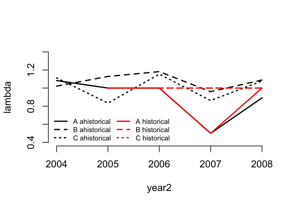
Figure 9.1: Lambda of ahistorical vs. historical raw MPMs
\(\lambda\) is quite different between the ahistorical and historical cases in the raw MPMs. This should give us pause and encourage us to consider using historical approaches to correct for the influence of individual history.
We may now wish to compare \(\lambda\) for the mean matrices, as well. Let’s do so, as below.
cyp2r_mean <- lmean(cypmatrix2r)
cyp2rp_mean <- lmean(cypmatrix2rp)
cyp3r_mean <- lmean(cypmatrix3r)
cyp3rp_mean <- lmean(cypmatrix3rp)

# Overall raw ahistorical lambda
lambda3(cyp2r_mean)
>   pop patch   lambda
> 1   1     1 1.082189

# Raw ahistorical lambda by patch
lambda3(cyp2rp_mean)
>   pop patch    lambda
> 1   1     A 0.9835717
> 2   1     B 1.1051470
> 3   1     C 1.0717513
> 4   1     0 1.0450267

# Overall raw historical lambda
lambda3(cyp3r_mean)
>   pop patch   lambda
> 1   1     1 1.011018

# Raw historical lambda by patch
lambda3(cyp3rp_mean)
>   pop patch    lambda
> 1   1     A 0.8510445
> 2   1     B 0.9481901
> 3   1     C 0.9671030
> 4   1     0 0.8946030
As we saw before, our historical estimates are lower than our ahistorical estimates. We also see that \(\lambda\) for the patch-weighted mean matrix (marked as patch 0 in the patch-level output) is lower than the whole-population \(\lambda\) in both ahistorical and historical cases. The latter result suggests that the patches have different levels of influence on overall population dynamics because of different numbers of individuals.
9.2 Stable stage distribution and reproductive value
The stable stage distribution is a vector showing the expected proportion of the population composed of each stage after we have projected the population forward in time sufficiently to create asymptotic conditions. The reproductive value vector gives the expected asymptotic contribution of an individual in each stage to future generations, and so has a relationship to natural selection (Caswell 2001). In ahistorical analysis, the stable stage distribution and the reproductive value vector are estimated as the standardized right and left eigenvectors, respectively, associated with the dominant eigenvalue of the matrix. Standardization of the stable stage distribution is handled by dividing each respective element of the right eigenvector by the sum of the elements in that eigenvector, yielding a vector that sums to 1.0. Standardization of the reproductive value vector is handled by dividing each element in the left eigenvector by the value of the first non-zero element in that eigenvector, which is also often though not always the lowest value. These estimation procedures make a number of key assumptions, and we urge users to read Caswell (2001) for further details.
The methods mentioned above apply to historical matrices as well (deVries & Caswell 2018). However, as described, these methods only provide the stable stage distribution and reproductive values of stage pairs, since each row and column in a historical matrix corresponds to a stage pair rather than an individual stage. We provide two functions, stablestage3() and repvalue3() to allow the estimation of these vectors for both ahistorical and historical MPMs. When provided with a historical MPM, these functions also estimate historically-corrected stable stage distributions and reproductive value vectors, which provide the stable stage distribution and reproductive value vector for the original stages in the associated life history model corrected for individual history. These vectors are comparable to ahistorical stable stage distributions and reproductive value vectors, though they should not be equal if individual history impacts population dynamics. The historically-corrected stable stage proportion for stage j is estimated as the sum of all stable stage proportions for stage \(j\) in occasion t across all stages in occasion t-1.
\[\begin{equation} SS _j = \sum _{l=1}^{m} w _{jl} \tag{9.4} \end{equation}\]
Here, \(l\) is stage in occasion t-1, \(m\) is the number of stages, \(SS_j\) is the stable stage proportion of stage \(j\), and \(w _{jl}\) is the stable stage proportion of stage pair \(jl\) given as the standardized right eigenvector corresponding to the dominant eigenvalue of the hMPM.
The historically-corrected reproductive value of stage \(j\) is calculated as the sum of all reproductive values for stage j in occasion t across all stages in occasion t-1, weighted by the stable stage proportion of the respective stage pair divided by the stable stage proportion of stage \(j\) in occasion t (Ehrlén 2000).
\[\begin{equation} RV _j = \sum _{l=1}^{m} v _{jl} (w _{jl} / SS _{j}) \tag{9.5} \end{equation}\]
Here, \(RV _j\) refers to the reproductive value of stage \(j\), and \(v _{jl}\) refers to the reproductive value of the stage pair as given by the standardized left eigenvector of the dominant eigenvalue of the historical MPM. Individual history can alter the stable stage distribution and reproductive value vector quite drastically from the ahistorical expectation.
Now let’s take a look at the stable stage distributions at the population level. We will start by looking just at the ahistorical equilibrium.
tm2ss_r <- stablestage3(cyp2r_mean)
tm2ss_r
>    matrix stage_id stage      ss_prop
> 1       1        1    SD 4.709506e-01
> 2       1        2    P1 4.796543e-01
> 3       1        3    P2 4.432261e-02
> 4       1        4    P3 4.095645e-03
> 5       1        5    SL 1.983961e-04
> 6       1        6  Dorm 4.309986e-05
> 7       1        7   XSm 2.759814e-04
> 8       1        8    Sm 3.049081e-04
> 9       1        9    Md 9.705559e-05
> 10      1       10    Lg 4.938104e-05
> 11      1       11   XLg 8.078062e-06
The output shows us the stage information and corresponding equilibrial proportion (ss_prop) for each matrix, of which there is only one. For each matrix, the proportions should sum to 1.0. Here, it appears that 48% of the stable stage structure is 1st year protocorms, and 47% is composed of dormant seeds, with most of the remaining 5% comprised of 2nd year protocorms.
Now let’s compare this output to the historical case.
tm3ss_r <- stablestage3(cyp3r_mean)
tm3ss_r
> $hist
>     matrix stage_id_2 stage_id_1 stage_2 stage_1      ss_prop
> 1        1          1          1      SD      SD 4.588724e-02
> 2        1          2          1      P1      SD 4.679498e-02
> 3        1          3          1      P2      SD 0.000000e+00
> 4        1          4          1      P3      SD 0.000000e+00
> 5        1          5          1      SL      SD 0.000000e+00
> 6        1          6          1    Dorm      SD 0.000000e+00
> 7        1          7          1     XSm      SD 0.000000e+00
> 8        1          8          1      Sm      SD 0.000000e+00
> 9        1          9          1      Md      SD 0.000000e+00
> 10       1         10          1      Lg      SD 0.000000e+00
> 11       1         11          1     XLg      SD 0.000000e+00
> 12       1          1          2      SD      P1 0.000000e+00
> 13       1          2          2      P1      P1 0.000000e+00
> 14       1          3          2      P2      P1 4.688477e-02
> 15       1          4          2      P3      P1 0.000000e+00
> 16       1          5          2      SL      P1 0.000000e+00
> 17       1          6          2    Dorm      P1 0.000000e+00
> 18       1          7          2     XSm      P1 0.000000e+00
> 19       1          8          2      Sm      P1 0.000000e+00
> 20       1          9          2      Md      P1 0.000000e+00
> 21       1         10          2      Lg      P1 0.000000e+00
> 22       1         11          2     XLg      P1 0.000000e+00
> 23       1          1          3      SD      P2 0.000000e+00
> 24       1          2          3      P1      P2 0.000000e+00
> 25       1          3          3      P2      P2 0.000000e+00
> 26       1          4          3      P3      P2 4.637381e-03
> 27       1          5          3      SL      P2 0.000000e+00
> 28       1          6          3    Dorm      P2 0.000000e+00
> 29       1          7          3     XSm      P2 0.000000e+00
> 30       1          8          3      Sm      P2 0.000000e+00
> 31       1          9          3      Md      P2 0.000000e+00
> 32       1         10          3      Lg      P2 0.000000e+00
> 33       1         11          3     XLg      P2 0.000000e+00
> 34       1          1          4      SD      P3 0.000000e+00
> 35       1          2          4      P1      P3 0.000000e+00
> 36       1          3          4      P2      P3 0.000000e+00
> 37       1          4          4      P3      P3 0.000000e+00
> 38       1          5          4      SL      P3 2.293422e-04
> 39       1          6          4    Dorm      P3 0.000000e+00
> 40       1          7          4     XSm      P3 0.000000e+00
> 41       1          8          4      Sm      P3 0.000000e+00
> 42       1          9          4      Md      P3 0.000000e+00
> 43       1         10          4      Lg      P3 0.000000e+00
> 44       1         11          4     XLg      P3 0.000000e+00
> 45       1          1          5      SD      SL 0.000000e+00
> 46       1          2          5      P1      SL 0.000000e+00
> 47       1          3          5      P2      SL 0.000000e+00
> 48       1          4          5      P3      SL 0.000000e+00
> 49       1          5          5      SL      SL 1.193225e-05
> 50       1          6          5    Dorm      SL 2.075488e-05
> 51       1          7          5     XSm      SL 9.455403e-05
> 52       1          8          5      Sm      SL 3.241594e-05
> 53       1          9          5      Md      SL 0.000000e+00
> 54       1         10          5      Lg      SL 0.000000e+00
> 55       1         11          5     XLg      SL 0.000000e+00
> 56       1          1          6      SD    Dorm 0.000000e+00
> 57       1          2          6      P1    Dorm 0.000000e+00
> 58       1          3          6      P2    Dorm 0.000000e+00
> 59       1          4          6      P3    Dorm 0.000000e+00
> 60       1          5          6      SL    Dorm 0.000000e+00
> 61       1          6          6    Dorm    Dorm 1.952294e-06
> 62       1          7          6     XSm    Dorm 3.097439e-05
> 63       1          8          6      Sm    Dorm 2.853934e-05
> 64       1          9          6      Md    Dorm 0.000000e+00
> 65       1         10          6      Lg    Dorm 1.952294e-06
> 66       1         11          6     XLg    Dorm 0.000000e+00
> 67       1          1          7      SD     XSm 1.585917e-02
> 68       1          2          7      P1     XSm 1.585917e-02
> 69       1          3          7      P2     XSm 0.000000e+00
> 70       1          4          7      P3     XSm 0.000000e+00
> 71       1          5          7      SL     XSm 0.000000e+00
> 72       1          6          7    Dorm     XSm 4.039813e-05
> 73       1          7          7     XSm     XSm 2.341842e-04
> 74       1          8          7      Sm     XSm 1.255182e-04
> 75       1          9          7      Md     XSm 6.421039e-06
> 76       1         10          7      Lg     XSm 0.000000e+00
> 77       1         11          7     XLg     XSm 0.000000e+00
> 78       1          1          8      SD      Sm 1.825976e-01
> 79       1          2          8      P1      Sm 1.825976e-01
> 80       1          3          8      P2      Sm 0.000000e+00
> 81       1          4          8      P3      Sm 0.000000e+00
> 82       1          5          8      SL      Sm 0.000000e+00
> 83       1          6          8    Dorm      Sm 2.368566e-05
> 84       1          7          8     XSm      Sm 1.114763e-04
> 85       1          8          8      Sm      Sm 2.007491e-04
> 86       1          9          8      Md      Sm 4.149712e-05
> 87       1         10          8      Lg      Sm 4.401622e-06
> 88       1         11          8     XLg      Sm 0.000000e+00
> 89       1          1          9      SD      Md 1.909135e-01
> 90       1          2          9      P1      Md 1.909135e-01
> 91       1          3          9      P2      Md 0.000000e+00
> 92       1          4          9      P3      Md 0.000000e+00
> 93       1          5          9      SL      Md 0.000000e+00
> 94       1          6          9    Dorm      Md 0.000000e+00
> 95       1          7          9     XSm      Md 1.004197e-05
> 96       1          8          9      Sm      Md 2.949146e-05
> 97       1          9          9      Md      Md 6.204565e-05
> 98       1         10          9      Lg      Md 5.996768e-06
> 99       1         11          9     XLg      Md 0.000000e+00
> 100      1          1         10      SD      Lg 3.337106e-02
> 101      1          2         10      P1      Lg 3.337106e-02
> 102      1          3         10      P2      Lg 0.000000e+00
> 103      1          4         10      P3      Lg 0.000000e+00
> 104      1          5         10      SL      Lg 0.000000e+00
> 105      1          6         10    Dorm      Lg 0.000000e+00
> 106      1          7         10     XSm      Lg 0.000000e+00
> 107      1          8         10      Sm      Lg 1.194258e-06
> 108      1          9         10      Md      Lg 2.677112e-06
> 109      1         10         10      Lg      Lg 5.257711e-06
> 110      1         11         10     XLg      Lg 6.918967e-07
> 111      1          1         11      SD     XLg 4.477104e-03
> 112      1          2         11      P1     XLg 4.477104e-03
> 113      1          3         11      P2     XLg 0.000000e+00
> 114      1          4         11      P3     XLg 0.000000e+00
> 115      1          5         11      SL     XLg 0.000000e+00
> 116      1          6         11    Dorm     XLg 0.000000e+00
> 117      1          7         11     XSm     XLg 0.000000e+00
> 118      1          8         11      Sm     XLg 0.000000e+00
> 119      1          9         11      Md     XLg 0.000000e+00
> 120      1         10         11      Lg     XLg 1.692245e-07
> 121      1         11         11     XLg     XLg 3.421782e-07
>
> $ahist
>    matrix stage_id stage      ss_prop
> 1       1        1    SD 4.731057e-01
> 2       1        2    P1 4.740135e-01
> 3       1        3    P2 4.688477e-02
> 4       1        4    P3 4.637381e-03
> 5       1        5    SL 2.412744e-04
> 6       1        6  Dorm 8.679096e-05
> 7       1        7   XSm 4.812309e-04
> 8       1        8    Sm 4.179082e-04
> 9       1        9    Md 1.126409e-04
> 10      1       10    Lg 1.777762e-05
> 11      1       11   XLg 1.034075e-06
We see two data frames, the first covering the expected equilibrial distribution of stage pairs, and the second showing the corrected equilibrial stage distribution. In both cases, the proportions sum to 1.0 within each matrix, of which there is only one. The amount of information here is difficult to digest at one glance, so let’s compare the ahistorical stage distribution to the historically corrected stage distribution via a bar plot (figure 9.2).
ss_put_together <- cbind.data.frame(tm2ss_r$ss_prop, tm3ss_r$ahist$ss_prop)
names(ss_put_together) <- c("ahistorical", "historical")
rownames(ss_put_together) <- tm2ss_r$stage

barplot(t(ss_put_together), beside=T, ylab = "Proportion", xlab = "Stage",
  ylim = c(0, 0.85), col = c("black", "orangered"), bty = "n")
legend("topright", c("ahistorical", "historical"), col = c("black","orangered"),
  pch = 15, cex = 0.9, bty = "n")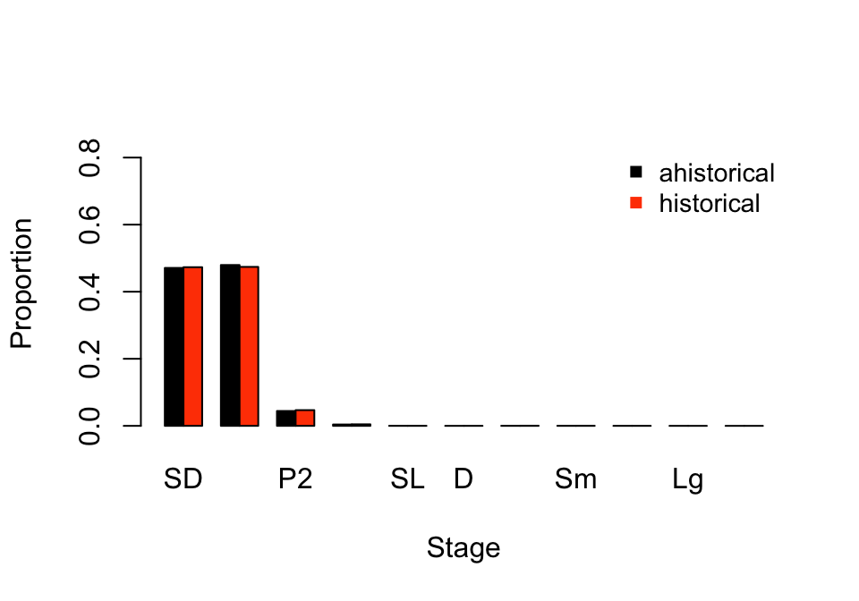
Figure 9.2: Ahistorical vs. historically-corrected stable stage distribution
Overall, these are very similar patterns. Particularly, both ahistorical and historical analyses suggest that dormant seeds and 1st year protocorms take up the greatest share of the stable stage structure, with 2nd year protocorms coming next. Adults contribute little to the stable stage structure. However, the historical model predicts a slightly greater share of the population composed of dormant seeds and 2nd year protocorms, and a slightly lower share composed of 1st year protocorms.
Next let’s look at the reproductive values associated with both ahistorical and historical approaches. We will initially look at just the ahistorical case.
tm2rv_r <- repvalue3(cyp2r_mean)
tm2rv_r
>    matrix stage_id stage    rep_value
> 1       1        1    SD      1.00000
> 2       1        2    P1     10.02189
> 3       1        3    P2    108.45573
> 4       1        4    P3   1173.69567
> 5       1        5    SL  25403.20404
> 6       1        6  Dorm  39100.90885
> 7       1        7   XSm  37601.08685
> 8       1        8    Sm  55396.33397
> 9       1        9    Md  85190.53793
> 10      1       10    Lg 128406.01230
> 11      1       11   XLg 179758.08291
We have a wide range in reproductive values among the stages, with the smallest value for dormant seeds and the largest for extra large adults. Note that the reproductive value vector is the left eigenvector divided by its first non-zero element, which here is the dormant seed stage. This strongly suggests that the largest adults have a disproportionately large impact on future generations.
Let’s now look at the historical reproductive values.
tm3rv_r <- repvalue3(cyp3r_mean)
tm3rv_r
> $hist
>     matrix stage_id_2 stage_id_1 stage_2 stage_1    rep_value
> 1        1          1          1      SD      SD 1.000000e+00
> 2        1          2          1      P1      SD 9.310181e+00
> 3        1          3          1      P2      SD 0.000000e+00
> 4        1          4          1      P3      SD 0.000000e+00
> 5        1          5          1      SL      SD 0.000000e+00
> 6        1          6          1    Dorm      SD 0.000000e+00
> 7        1          7          1     XSm      SD 0.000000e+00
> 8        1          8          1      Sm      SD 0.000000e+00
> 9        1          9          1      Md      SD 0.000000e+00
> 10       1         10          1      Lg      SD 0.000000e+00
> 11       1         11          1     XLg      SD 0.000000e+00
> 12       1          1          2      SD      P1 0.000000e+00
> 13       1          2          2      P1      P1 0.000000e+00
> 14       1          3          2      P2      P1 9.412762e+01
> 15       1          4          2      P3      P1 0.000000e+00
> 16       1          5          2      SL      P1 0.000000e+00
> 17       1          6          2    Dorm      P1 0.000000e+00
> 18       1          7          2     XSm      P1 0.000000e+00
> 19       1          8          2      Sm      P1 0.000000e+00
> 20       1          9          2      Md      P1 0.000000e+00
> 21       1         10          2      Lg      P1 0.000000e+00
> 22       1         11          2     XLg      P1 0.000000e+00
> 23       1          1          3      SD      P2 0.000000e+00
> 24       1          2          3      P1      P2 0.000000e+00
> 25       1          3          3      P2      P2 0.000000e+00
> 26       1          4          3      P3      P2 9.516473e+02
> 27       1          5          3      SL      P2 0.000000e+00
> 28       1          6          3    Dorm      P2 0.000000e+00
> 29       1          7          3     XSm      P2 0.000000e+00
> 30       1          8          3      Sm      P2 0.000000e+00
> 31       1          9          3      Md      P2 0.000000e+00
> 32       1         10          3      Lg      P2 0.000000e+00
> 33       1         11          3     XLg      P2 0.000000e+00
> 34       1          1          4      SD      P3 0.000000e+00
> 35       1          2          4      P1      P3 0.000000e+00
> 36       1          3          4      P2      P3 0.000000e+00
> 37       1          4          4      P3      P3 0.000000e+00
> 38       1          5          4      SL      P3 1.924265e+04
> 39       1          6          4    Dorm      P3 0.000000e+00
> 40       1          7          4     XSm      P3 0.000000e+00
> 41       1          8          4      Sm      P3 0.000000e+00
> 42       1          9          4      Md      P3 0.000000e+00
> 43       1         10          4      Lg      P3 0.000000e+00
> 44       1         11          4     XLg      P3 0.000000e+00
> 45       1          1          5      SD      SL 0.000000e+00
> 46       1          2          5      P1      SL 0.000000e+00
> 47       1          3          5      P2      SL 0.000000e+00
> 48       1          4          5      P3      SL 0.000000e+00
> 49       1          5          5      SL      SL 1.924265e+04
> 50       1          6          5    Dorm      SL 1.600483e+04
> 51       1          7          5     XSm      SL 2.685861e+04
> 52       1          8          5      Sm      SL 4.755014e+04
> 53       1          9          5      Md      SL 0.000000e+00
> 54       1         10          5      Lg      SL 0.000000e+00
> 55       1         11          5     XLg      SL 0.000000e+00
> 56       1          1          6      SD    Dorm 0.000000e+00
> 57       1          2          6      P1    Dorm 0.000000e+00
> 58       1          3          6      P2    Dorm 0.000000e+00
> 59       1          4          6      P3    Dorm 0.000000e+00
> 60       1          5          6      SL    Dorm 0.000000e+00
> 61       1          6          6    Dorm    Dorm 4.034282e+03
> 62       1          7          6     XSm    Dorm 1.631493e+04
> 63       1          8          6      Sm    Dorm 2.683487e+04
> 64       1          9          6      Md    Dorm 0.000000e+00
> 65       1         10          6      Lg    Dorm 3.449945e+04
> 66       1         11          6     XLg    Dorm 0.000000e+00
> 67       1          1          7      SD     XSm 1.019782e+00
> 68       1          2          7      P1     XSm 9.310181e+00
> 69       1          3          7      P2     XSm 0.000000e+00
> 70       1          4          7      P3     XSm 0.000000e+00
> 71       1          5          7      SL     XSm 0.000000e+00
> 72       1          6          7    Dorm     XSm 1.600483e+04
> 73       1          7          7     XSm     XSm 2.728434e+04
> 74       1          8          7      Sm     XSm 5.010449e+04
> 75       1          9          7      Md     XSm 6.833780e+04
> 76       1         10          7      Lg     XSm 1.518934e+04
> 77       1         11          7     XLg     XSm 0.000000e+00
> 78       1          1          8      SD      Sm 1.019782e+00
> 79       1          2          8      P1      Sm 9.310181e+00
> 80       1          3          8      P2      Sm 0.000000e+00
> 81       1          4          8      P3      Sm 0.000000e+00
> 82       1          5          8      SL      Sm 0.000000e+00
> 83       1          6          8    Dorm      Sm 1.519080e+04
> 84       1          7          8     XSm      Sm 3.623157e+04
> 85       1          8          8      Sm      Sm 7.229060e+04
> 86       1          9          8      Md      Sm 1.037423e+05
> 87       1         10          8      Lg      Sm 1.421550e+04
> 88       1         11          8     XLg      Sm 0.000000e+00
> 89       1          1          9      SD      Md 1.019782e+00
> 90       1          2          9      P1      Md 9.310181e+00
> 91       1          3          9      P2      Md 0.000000e+00
> 92       1          4          9      P3      Md 0.000000e+00
> 93       1          5          9      SL      Md 0.000000e+00
> 94       1          6          9    Dorm      Md 0.000000e+00
> 95       1          7          9     XSm      Md 4.524192e+04
> 96       1          8          9      Sm      Md 6.755724e+04
> 97       1          9          9      Md      Md 1.381815e+05
> 98       1         10          9      Lg      Md 8.161812e+04
> 99       1         11          9     XLg      Md 0.000000e+00
> 100      1          1         10      SD      Lg 1.019782e+00
> 101      1          2         10      P1      Lg 9.310181e+00
> 102      1          3         10      P2      Lg 0.000000e+00
> 103      1          4         10      P3      Lg 0.000000e+00
> 104      1          5         10      SL      Lg 0.000000e+00
> 105      1          6         10    Dorm      Lg 0.000000e+00
> 106      1          7         10     XSm      Lg 0.000000e+00
> 107      1          8         10      Sm      Lg 5.355023e+04
> 108      1          9         10      Md      Lg 6.142678e+04
> 109      1         10         10      Lg      Lg 1.395183e+05
> 110      1         11         10     XLg      Lg 8.345149e+04
> 111      1          1         11      SD     XLg 1.019782e+00
> 112      1          2         11      P1     XLg 9.310181e+00
> 113      1          3         11      P2     XLg 0.000000e+00
> 114      1          4         11      P3     XLg 0.000000e+00
> 115      1          5         11      SL     XLg 0.000000e+00
> 116      1          6         11    Dorm     XLg 0.000000e+00
> 117      1          7         11     XSm     XLg 0.000000e+00
> 118      1          8         11      Sm     XLg 0.000000e+00
> 119      1          9         11      Md     XLg 0.000000e+00
> 120      1         10         11      Lg     XLg 6.790669e+04
> 121      1         11         11     XLg     XLg 7.189852e+04
>
> $ahist
>    matrix stage_id stage    rep_value
> 1       1        1    SD 1.000000e+00
> 2       1        2    P1 9.146789e+00
> 3       1        3    P2 9.247569e+01
> 4       1        4    P3 9.349460e+02
> 5       1        5    SL 1.890495e+04
> 6       1        6  Dorm 1.524115e+04
> 7       1        7   XSm 2.843405e+04
> 8       1        8    Sm 5.915940e+04
> 9       1        9    Md 1.175879e+05
> 10      1       10    Lg 7.540168e+04
> 11      1       11   XLg 7.823111e+04
As in the stable stage output, we see two data frames. The first shows the reproductive values of historical stage pairs, which have been standardized by dividing the left eigenvector by its minimum element. Most reproductive values are zero, generally when referring to an impossible stage pairing (e.g. an individual cannot be a small adult in one year and a 3rd year protocorm in the next). The biologically possible pairs are generally positive. The second data frame shows historically-corrected reproductive values for each stage in the stageframe. Note that individual history has reduced the reproductive values of most stages. Let’s compare the ahistorical reproductive values to the historically-corrected reproductive values, in a side-by-side pair of plots (figure 9.3).
tm2rv_r <- repvalue3(cyp2r_mean)
tm3rv_r <- repvalue3(cyp3r_mean)

tm2rv_plot <- as.matrix(tm2rv_r$rep_value)
rownames(tm2rv_plot) <- tm2rv_r$stage

tm3rv_plot <- as.matrix(tm3rv_r$ahist$rep_value)
rownames(tm3rv_plot) <- tm3rv_r$ahist$stage

par(mfrow=c(1,2))
barplot(t(tm2rv_plot), ylab = "Rep value", xlab = "Stage", col = "black",
  ylim = c(0, 200000), bty = "n")
title("a)", adj = 0)
legend("topleft", c("ahistorical", "historical"), col = c("black", "orangered"),
  pch = 15, bty = "n")

barplot(t(tm3rv_plot), ylab = "", xlab = "Stage", col = "orangered",
  ylim = c(0, 200000), bty = "n")
title("b)", adj = 0)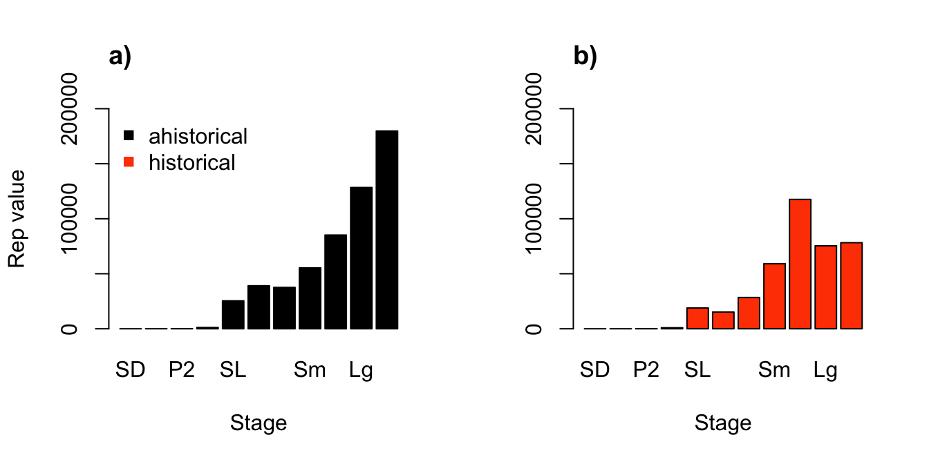
Figure 9.3: Ahistorical (a) vs. historically-corrected (b) deterministic reproductive values
We see some big differences here. In the ahistorical case, reproductive value increased with size, reaching its peak in the largest adults. In contrast, in the historical case, the greatest reproductive values were associated with medium adults, decreasing again in large and extra large adults. So, history appears to have had large effects here. Given that reproductive value has implications for natural selection, we might hypothesize that size-related traits might evolve differently under these two models. Interesting results in need of further study!
9.3 Sensitivity analysis
Package lefko3 contains functions allowing users to conduct deterministic and stochastic sensitivity and elasticity analyses. Sensitivity and elasticity analysis are forms of perturbation analysis, and we urge readers to consult Caswell (2001) and Caswell (2019) to become fully acquainted with the topic. Here, we discuss just the most important aspects to understand these analyses as conducted using lefko3.
The sensitivity of \(\lambda\), the deterministic population growth rate, to a specific element in a projection matrix can be calculated using eigenanalysis, as below.
\[\begin{equation} \frac{\partial \lambda}{\partial a _{kj}} = \frac{\bar{v} _{k} w _{j}}{<\mathbf{w}, \mathbf{v}>} \tag{9.6} \end{equation}\]
Here, \(\mathbf{w}\) is the stable stage distribution vector calculated as the right eigenvector of the dominant eigenvalue of the matrix (standardized to sum to 1.0), \(\mathbf{v}\) is the reproductive value vector calculated as the associated left eigenvector (standardized by dividing by the value of the first non-zero or minimum value), \(w _{j}\) is element \(j\) of the stable stage distribution vector, and \(\bar{v} _{k}\) is the complex conjugate of element \(k\) of \(\mathbf{v}\). \(k\) refers to stage in occasion t+1 and in the ahMPM refers to the corresponding row, while \(j\) refers to stage in occasion t and in an ahMPM refers to the corresponding column. The term \(<\mathbf{w}, \mathbf{v}>\) refers to the scalar product of these vectors.
In the hMPM case, the basic method is essentially the same, although the equation itself changes somewhat to account for stage \(l\) in occasion t-1. Thus, the sensitivity of \(\lambda\) to each matrix element in an hMPM is given as
\[\begin{equation} \frac{\partial \lambda}{\partial a _{kjl}} = \frac{\bar{v} _{kj} w _{jl}}{<\mathbf{w}, \mathbf{v}>} \tag{9.7} \end{equation}\]
Here, \(k\) and \(j\) are as before, \(l\) is stage in occasion t-1, \(kj\) refers both to the stage pair in occasions t+1 and t as well as the corresponding row in the historical matrix, and \(jl\) refers both to the stage pair in occasions t and t-1 as well as the corresponding column in the historical matrix. Historically-corrected sensitivities may also be estimated for the basic stages of the life history model using the historically-corrected stable stage distributions and reproductive values given in equations (9.4) and (9.5).
Let’s analyze the sensitivity of \(\lambda\) to the elements of our raw Cypripedium candidum MPMs. First, let’s look at the raw ahistorical MPM.
tm2sens_r <- sensitivity3(cyp2r_mean)
> Running deterministic analysis...
tm2sens_r
> $h_sensmats
> NULL
>
> $ah_sensmats
> $ah_sensmats[[1]]
>               [,1]         [,2]         [,3]         [,4]         [,5]
>  [1,] 7.251380e-03 7.385393e-03 6.824496e-04 6.306198e-05 3.054770e-06
>  [2,] 7.267251e-02 7.401557e-02 6.839433e-03 6.320001e-04 3.061456e-05
>  [3,] 7.864537e-01 8.009882e-01 7.401557e-02 6.839433e-03 3.313073e-04
>  [4,] 8.510913e+00 8.668204e+00 8.009882e-01 7.401557e-02 3.585370e-03
>  [5,] 1.842083e+02 1.876126e+02 1.733641e+01 1.601976e+00 7.760094e-02
>  [6,] 2.835355e+02 2.887756e+02 2.668440e+01 2.465781e+00 1.194443e-01
>  [7,] 2.726598e+02 2.776988e+02 2.566085e+01 2.371199e+00 1.148627e-01
>  [8,] 4.016999e+02 4.091237e+02 3.780521e+01 3.493403e+00 1.692231e-01
>  [9,] 6.177489e+02 6.291656e+02 5.813825e+01 5.372284e+00 2.602375e-01
> [10,] 9.311208e+02 9.483289e+02 8.763064e+01 8.097538e+00 3.922508e-01
> [11,] 1.303494e+03 1.327584e+03 1.226758e+02 1.133590e+01 5.491196e-01
>               [,6]         [,7]         [,8]         [,9]        [,10]
>  [1,] 6.636226e-07 4.249376e-06 4.694769e-06 1.494397e-06 7.603360e-07
>  [2,] 6.650750e-06 4.258676e-05 4.705044e-05 1.497667e-05 7.620002e-06
>  [3,] 7.197367e-05 4.608692e-04 5.091746e-04 1.620759e-04 8.246280e-05
>  [4,] 7.788909e-04 4.987474e-03 5.510230e-03 1.753967e-03 8.924031e-04
>  [5,] 1.685814e-02 1.079478e-01 1.192622e-01 3.796246e-02 1.931497e-02
>  [6,] 2.594825e-02 1.661545e-01 1.835697e-01 5.843227e-02 2.972983e-02
>  [7,] 2.495293e-02 1.597811e-01 1.765284e-01 5.619094e-02 2.858946e-02
>  [8,] 3.676226e-02 2.353998e-01 2.600730e-01 8.278409e-02 4.211983e-02
>  [9,] 5.653436e-02 3.620066e-01 3.999499e-01 1.273085e-01 6.477344e-02
> [10,] 8.521313e-02 5.456454e-01 6.028365e-01 1.918895e-01 9.763172e-02
> [11,] 1.192915e-01 7.638596e-01 8.439226e-01 2.686299e-01 1.366765e-01
>              [,11]
>  [1,] 1.243806e-07
>  [2,] 1.246528e-06
>  [3,] 1.348978e-05
>  [4,] 1.459849e-04
>  [5,] 3.159665e-03
>  [6,] 4.863393e-03
>  [7,] 4.676844e-03
>  [8,] 6.890227e-03
>  [9,] 1.059605e-02
> [10,] 1.597121e-02
> [11,] 2.235841e-02
>
>
> $hstages
> NULL
>
> $ahstages
>    stage_id stage original_size original_size_b original_size_c min_age max_age
> 1         1    SD           0.0              NA              NA       0      NA
> 2         2    P1           0.0              NA              NA       0      NA
> 3         3    P2           0.0              NA              NA       0      NA
> 4         4    P3           0.0              NA              NA       0      NA
> 5         5    SL           0.0              NA              NA       0      NA
> 6         6  Dorm           0.0              NA              NA       0      NA
> 7         7   XSm           1.0              NA              NA       0      NA
> 8         8    Sm           3.0              NA              NA       0      NA
> 9         9    Md           6.0              NA              NA       0      NA
> 10       10    Lg          11.0              NA              NA       0      NA
> 11       11   XLg          19.5              NA              NA       0      NA
>    repstatus obsstatus propstatus immstatus matstatus entrystage indataset
> 1          0         0          1         0         0          1         0
> 2          0         0          0         1         0          1         0
> 3          0         0          0         1         0          0         0
> 4          0         0          0         1         0          0         0
> 5          0         0          0         1         0          0         0
> 6          0         0          0         0         1          0         1
> 7          1         1          0         0         1          0         1
> 8          1         1          0         0         1          0         1
> 9          1         1          0         0         1          0         1
> 10         1         1          0         0         1          0         1
> 11         1         1          0         0         1          0         1
>    binhalfwidth_raw sizebin_min sizebin_max sizebin_center sizebin_width
> 1               0.0         0.0         0.0            0.0             0
> 2               0.0         0.0         0.0            0.0             0
> 3               0.0         0.0         0.0            0.0             0
> 4               0.0         0.0         0.0            0.0             0
> 5               0.0         0.0         0.0            0.0             0
> 6               0.5        -0.5         0.5            0.0             1
> 7               0.5         0.5         1.5            1.0             1
> 8               1.5         1.5         4.5            3.0             3
> 9               1.5         4.5         7.5            6.0             3
> 10              3.5         7.5        14.5           11.0             7
> 11              5.0        14.5        24.5           19.5            10
>    binhalfwidthb_raw sizebinb_min sizebinb_max sizebinb_center sizebinb_width
> 1                 NA           NA           NA              NA             NA
> 2                 NA           NA           NA              NA             NA
> 3                 NA           NA           NA              NA             NA
> 4                 NA           NA           NA              NA             NA
> 5                 NA           NA           NA              NA             NA
> 6                 NA           NA           NA              NA             NA
> 7                 NA           NA           NA              NA             NA
> 8                 NA           NA           NA              NA             NA
> 9                 NA           NA           NA              NA             NA
> 10                NA           NA           NA              NA             NA
> 11                NA           NA           NA              NA             NA
>    binhalfwidthc_raw sizebinc_min sizebinc_max sizebinc_center sizebinc_width
> 1                 NA           NA           NA              NA             NA
> 2                 NA           NA           NA              NA             NA
> 3                 NA           NA           NA              NA             NA
> 4                 NA           NA           NA              NA             NA
> 5                 NA           NA           NA              NA             NA
> 6                 NA           NA           NA              NA             NA
> 7                 NA           NA           NA              NA             NA
> 8                 NA           NA           NA              NA             NA
> 9                 NA           NA           NA              NA             NA
> 10                NA           NA           NA              NA             NA
> 11                NA           NA           NA              NA             NA
>    group                       comments alive almostborn
> 1      0                   Dormant seed     1          0
> 2      0               1st yr protocorm     1          0
> 3      0               2nd yr protocorm     1          0
> 4      0               3rd yr protocorm     1          0
> 5      0                       Seedling     1          0
> 6      0                  Dormant adult     1          0
> 7      0    Extra small adult (1 shoot)     1          0
> 8      0       Small adult (2-4 shoots)     1          0
> 9      0      Medium adult (5-7 shoots)     1          0
> 10     0      Large adult (8-14 shoots)     1          0
> 11     0 Extra large adult (>14 shoots)     1          0
>
> $agestages
>   X1
> 1 NA
>
> $labels
>   pop patch
> 1   1     1
>
> attr(,"class")
> [1] "lefkoSens"
The output is a list with several elements. The first element is called h_sensmats, and it would hold the sensitivity matrices of the \(\mathbf{A}\) matrices in the lefkoMat object input if our MPM was historical. Here, our MPM is actually ahistorical, so this element is empty. The second element, ah_sensmats, is a list of sensitivity matrices with each matrix corresponding to each matrix of our input MPM in order. If we had input a historical MPM, then this element would show matrices of the historically-corrected sensitivities. The order of stage pairs would be shown in element h_stages if the input MPM was historical. Element ah_stages always shows the stageframe underlying the MPM.
Sensitivity matrices can be hard to read, because all of the elements are estimated to have non-zero sensitivities even if the matrix element must equal zero. It usually helps to analyze such matrices with particular questions in mind. For example, what element is \(\lambda\) most sensitive to changes in? We can address this by using the matrix_interp() function, as below.
tm2sens_r_mi <- matrix_interp(tm2sens_r)
tm2sens_r_mi
>     index from_stage to_stage column row        value
> 1      22         P1      XLg      2  11 1.327584e+03
> 2      11         SD      XLg      1  11 1.303494e+03
> 3      21         P1       Lg      2  10 9.483289e+02
> 4      10         SD       Lg      1  10 9.311208e+02
> 5      20         P1       Md      2   9 6.291656e+02
> 6       9         SD       Md      1   9 6.177489e+02
> 7      19         P1       Sm      2   8 4.091237e+02
> 8       8         SD       Sm      1   8 4.016999e+02
> 9      17         P1     Dorm      2   6 2.887756e+02
> 10      6         SD     Dorm      1   6 2.835355e+02
> 11     18         P1      XSm      2   7 2.776988e+02
> 12      7         SD      XSm      1   7 2.726598e+02
> 13     16         P1       SL      2   5 1.876126e+02
> 14      5         SD       SL      1   5 1.842083e+02
> 15     33         P2      XLg      3  11 1.226758e+02
> 16     32         P2       Lg      3  10 8.763064e+01
> 17     31         P2       Md      3   9 5.813825e+01
> 18     30         P2       Sm      3   8 3.780521e+01
> 19     28         P2     Dorm      3   6 2.668440e+01
> 20     29         P2      XSm      3   7 2.566085e+01
> 21     27         P2       SL      3   5 1.733641e+01
> 22     44         P3      XLg      4  11 1.133590e+01
> 23     15         P1       P3      2   4 8.668204e+00
> 24      4         SD       P3      1   4 8.510913e+00
> 25     43         P3       Lg      4  10 8.097538e+00
> 26     42         P3       Md      4   9 5.372284e+00
> 27     41         P3       Sm      4   8 3.493403e+00
> 28     39         P3     Dorm      4   6 2.465781e+00
> 29     40         P3      XSm      4   7 2.371199e+00
> 30     38         P3       SL      4   5 1.601976e+00
> 31     88         Sm      XLg      8  11 8.439226e-01
> 32     26         P2       P3      3   4 8.009882e-01
> 33     14         P1       P2      2   3 8.009882e-01
> 34      3         SD       P2      1   3 7.864537e-01
> 35     77        XSm      XLg      7  11 7.638596e-01
> 36     87         Sm       Lg      8  10 6.028365e-01
> 37     55         SL      XLg      5  11 5.491196e-01
> 38     76        XSm       Lg      7  10 5.456454e-01
> 39     86         Sm       Md      8   9 3.999499e-01
> 40     54         SL       Lg      5  10 3.922508e-01
> 41     75        XSm       Md      7   9 3.620066e-01
> 42     99         Md      XLg      9  11 2.686299e-01
> 43     53         SL       Md      5   9 2.602375e-01
> 44     85         Sm       Sm      8   8 2.600730e-01
> 45     74        XSm       Sm      7   8 2.353998e-01
> 46     98         Md       Lg      9  10 1.918895e-01
> 47     83         Sm     Dorm      8   6 1.835697e-01
> 48     84         Sm      XSm      8   7 1.765284e-01
> 49     52         SL       Sm      5   8 1.692231e-01
> 50     72        XSm     Dorm      7   6 1.661545e-01
> 51     73        XSm      XSm      7   7 1.597811e-01
> 52    110         Lg      XLg     10  11 1.366765e-01
> 53     97         Md       Md      9   9 1.273085e-01
> 54     50         SL     Dorm      5   6 1.194443e-01
> 55     66       Dorm      XLg      6  11 1.192915e-01
> 56     82         Sm       SL      8   5 1.192622e-01
> 57     51         SL      XSm      5   7 1.148627e-01
> 58     71        XSm       SL      7   5 1.079478e-01
> 59    109         Lg       Lg     10  10 9.763172e-02
> 60     65       Dorm       Lg      6  10 8.521313e-02
> 61     96         Md       Sm      9   8 8.278409e-02
> 62     49         SL       SL      5   5 7.760094e-02
> 63     13         P1       P1      2   2 7.401557e-02
> 64     37         P3       P3      4   4 7.401557e-02
> 65     25         P2       P2      3   3 7.401557e-02
> 66      2         SD       P1      1   2 7.267251e-02
> 67    108         Lg       Md     10   9 6.477344e-02
> 68     94         Md     Dorm      9   6 5.843227e-02
> 69     64       Dorm       Md      6   9 5.653436e-02
> 70     95         Md      XSm      9   7 5.619094e-02
> 71    107         Lg       Sm     10   8 4.211983e-02
> 72     93         Md       SL      9   5 3.796246e-02
> 73     63       Dorm       Sm      6   8 3.676226e-02
> 74    105         Lg     Dorm     10   6 2.972983e-02
> 75    106         Lg      XSm     10   7 2.858946e-02
> 76     61       Dorm     Dorm      6   6 2.594825e-02
> 77     62       Dorm      XSm      6   7 2.495293e-02
> 78    121        XLg      XLg     11  11 2.235841e-02
> 79    104         Lg       SL     10   5 1.931497e-02
> 80     60       Dorm       SL      6   5 1.685814e-02
> 81    120        XLg       Lg     11  10 1.597121e-02
> 82    119        XLg       Md     11   9 1.059605e-02
> 83     12         P1       SD      2   1 7.385393e-03
> 84      1         SD       SD      1   1 7.251380e-03
> 85    118        XLg       Sm     11   8 6.890227e-03
> 86     24         P2       P1      3   2 6.839433e-03
> 87     36         P3       P2      4   3 6.839433e-03
> 88     81         Sm       P3      8   4 5.510230e-03
> 89     70        XSm       P3      7   4 4.987474e-03
> 90    116        XLg     Dorm     11   6 4.863393e-03
> 91    117        XLg      XSm     11   7 4.676844e-03
> 92     48         SL       P3      5   4 3.585370e-03
> 93    115        XLg       SL     11   5 3.159665e-03
> 94     92         Md       P3      9   4 1.753967e-03
> 95    103         Lg       P3     10   4 8.924031e-04
> 96     59       Dorm       P3      6   4 7.788909e-04
> 97     23         P2       SD      3   1 6.824496e-04
> 98     35         P3       P1      4   2 6.320001e-04
> 99     80         Sm       P2      8   3 5.091746e-04
> 100    69        XSm       P2      7   3 4.608692e-04
> 101    47         SL       P2      5   3 3.313073e-04
> 102    91         Md       P2      9   3 1.620759e-04
> 103   114        XLg       P3     11   4 1.459849e-04
> 104   102         Lg       P2     10   3 8.246280e-05
> 105    58       Dorm       P2      6   3 7.197367e-05
> 106    34         P3       SD      4   1 6.306198e-05
> 107    79         Sm       P1      8   2 4.705044e-05
> 108    68        XSm       P1      7   2 4.258676e-05
> 109    46         SL       P1      5   2 3.061456e-05
> 110    90         Md       P1      9   2 1.497667e-05
> 111   113        XLg       P2     11   3 1.348978e-05
> 112   101         Lg       P1     10   2 7.620002e-06
> 113    57       Dorm       P1      6   2 6.650750e-06
> 114    78         Sm       SD      8   1 4.694769e-06
> 115    67        XSm       SD      7   1 4.249376e-06
> 116    45         SL       SD      5   1 3.054770e-06
> 117    89         Md       SD      9   1 1.494397e-06
> 118   112        XLg       P1     11   2 1.246528e-06
> 119   100         Lg       SD     10   1 7.603360e-07
> 120    56       Dorm       SD      6   1 6.636226e-07
> 121   111        XLg       SD     11   1 1.243806e-07
The matrix_interp() function arranges matrix elements (including sensitivity matries) in order from greatest to smallest magnitude, by default. The output shows that the top sensitivity values all appear to be for impossible transitions. For example, it is impossible to move from 1st year protocorm (stage P1) to extra-large adult (stage XLg), because any individual in 1st year protocorm must move to 2nd year protocorm, 3rd year protocorm, and seedling first (stages P2, P3, and SL, respectively). In fact, the first biologically plausible transition in the output appears to be transition index 38 (row 30 above), which is the transition from 3rd year protocorm to seedling.
Because sensitivity analyses yield sensitivity values even for biologically impossible transitions, it is sometimes easier to use other means to see which transitions are the most important. Here, we use a different approach in which we look for the maximum sensitivity value among only those sensitivity matrix elements that do not correspond with zero values in the original MPM.
# The highest deterministic sensitivity value
max(tm2sens_r$ah_sensmats[[1]][which(cyp2r_mean$A[[1]] > 0)])
> [1] 1.601976

# This value is associated with element
max_sens <- intersect(which(tm2sens_r$ah_sensmats[[1]] ==
    max(tm2sens_r$ah_sensmats[[1]][which(cyp2r_mean$A[[1]] > 0)])),
  which(cyp2r_mean$A[[1]] > 0))
max_sens
> [1] 38

# This element is associated with column
ceiling(max_sens / dim(tm2sens_r$ahstages)[1])
> [1] 4
# and row
max_sens %% dim(tm2sens_r$ahstages)[1]
> [1] 5
We see confirmation of what we saw in the matrix_interp() output.
How does all of this compare with the historical sensitivity analysis? Let’s take a look, remembering that we will now get a historical sensitivity matrix with 121 rows and columns each corresponding to stage pairs, as well as a historically-corrected sensitivity matrix with 11 rows and columns each corresponding to stages.
tm3sens_r <- sensitivity3(cyp3r_mean)
> Running deterministic analysis...

# Highest sensitivity in the historical matrix
max(tm3sens_r$h_sensmats[[1]][which(cyp3r_mean$A[[1]] > 0)])
> [1] 1.210279

# This value is associated with element
max_sens1 <- intersect(which(tm3sens_r$h_sensmats[[1]] ==
        max(tm3sens_r$h_sensmats[[1]][which(cyp3r_mean$A[[1]] > 0)])),
  which(cyp3r_mean$A[[1]] > 0))
max_sens1
> [1] 3063

# This element is associated with column
ceiling(max_sens1 / dim(tm3sens_r$hstages)[1])
> [1] 26
# and row
max_sens1 %% dim(tm3sens_r$hstages)[1]
> [1] 38

# Highest sensitivity in the historically-corrected matrix
max(tm3sens_r$ah_sensmats[[1]][which(cyp2r_mean$A[[1]] > 0)])
> [1] 1.210279

# This value is associated with element
max_sens2 <- intersect(which(tm3sens_r$ah_sensmats[[1]] ==
      max(tm3sens_r$ah_sensmats[[1]][which(cyp2r_mean$A[[1]] > 0)])),
  which(cyp2r_mean$A[[1]] > 0))
max_sens2
> [1] 38

# This element is associated with column
ceiling(max_sens2 / dim(tm3sens_r$ahstages)[1])
> [1] 4
# and row
max_sens2 %% dim(tm3sens_r$ahstages)[1]
> [1] 5
Here we find that \(\lambda\) in the hMPM is most sensitive to element 3063. This corresponds to the transition from the 26th stage pair (2nd year protocorm in time t-1 and 3rd year protocorm in time t), to the 38th stage pair (3rd year protocorm in time t and seedling in time t+1). Further, the historically-corrected highest sensitivity is the same transition as in the ahistorical case. So, once again we find that early-life transitions have strong additive influences on \(\lambda\).
Incidentally, users may wish to know how we can easily understand which transition each matrix element corresponds to. For example, how do we know that element 3063 corresponds to the transition from the 26th stage pair to the 38th stage pair? The element index 3063 assumes a column vectorized matrix, meaning that we can think of the matrix as a column vector where the left-most column is stacked on top of the second column, and this combined vector is stacked on top of the third column, etc. In the historical matrix, there are 121 rows and columns, so to determine which column we are in, we need to divide the element index by the number of columns and round up to the nearest integer, as below.
To determine the row, we divide the matrix element index by the number of columns and take the remainder.
9.4 Elasticity analysis
Sensitivities show how much a small, additive change in a matrix element can alter \(\lambda\). They do so by estimating the local slope of \(\lambda\) given in terms of the matrix element (Caswell 2001). Problematically, sensitivities are also typically non-zero even for impossible transitions represented by zeros in the MPM. Elasticities, in contrast, show the influence of a small, proportional change in a matrix element on \(\lambda\), essentially given as the local slope of \(log \lambda\) given in terms of the log of the matrix element. This results in impossible transitions yielding elasticity values equal to zero, although it also yields somewhat different inferences from sensitivity analysis.
In the ahistorical case, the elasticity, \(e _{kj}\), of \(\lambda\) to change in a matrix element \(a _{kj}\) is given as the following.
\[\begin{equation} e _{kj} = \frac{a _{kj}}{\lambda} \frac{\partial \lambda}{\partial a _{kj}} \tag{9.8} \end{equation}\]
The historical case is just an extension of the above to include stage \(l\) in occasion t-1.
\[\begin{equation} e _{kjl} = \frac{a _{kjl}}{\lambda} \frac{\partial \lambda}{\partial a _{kjl}} \tag{9.9} \end{equation}\]
Here, we use row and column definitions equivalent to those used in the historical sensitivity case. The elasticity of \(\lambda\) to a specific matrix element is actually a function of the sensitivity of \(\lambda\) to that matrix element, as well as of the value of the matrix element itself. Thus, structural zeros in the hMPM must have elasticity equal to zero, although it is entirely possible that they have non-zero sensitivity values.
Elasticity values calculated for hMPMs can be compared to those calculated in ahMPMs easily because elasticities may be added by stage or transition type, with all elasticities corresponding to a specific matrix necessarily summing to 1.0. We can calculate the stage pair elasticities resulting from a historical MPM analysis in the following manner, with all symbol definitions as before.
\[\begin{equation} e _{kj} = \sum_{i=1}^{m} e _{kji} \tag{9.10} \end{equation}\]
These stage pair elasticity values are historically-corrected, and so can be added together in matrices of equivalent dimension to the ahistorical matrices and compared against the latter. We have provided a summary() function for elasticity output in lefko3 that automatically groups the resulting elasticity values by the kind of ahistorical or historical transition.
Let’s now assess the elasticity of \(\lambda\) to matrix elements in our MPMs, comparing the ahistorical to the historically-corrected case. We’ll start off by looking at the ahistorical case.
tm2elas_r <- elasticity3(cyp2r_mean)
> Running deterministic analysis...
tm2elas_r
> $h_elasmats
> NULL
>
> $ah_elasmats
> $ah_elasmats[[1]]
>               [,1]       [,2]       [,3]       [,4]        [,5]        [,6]
>  [1,] 0.0005360529 0.00000000 0.00000000 0.00000000 0.000000000 0.000000000
>  [2,] 0.0067153268 0.00000000 0.00000000 0.00000000 0.000000000 0.000000000
>  [3,] 0.0000000000 0.07401557 0.00000000 0.00000000 0.000000000 0.000000000
>  [4,] 0.0000000000 0.00000000 0.07401557 0.00000000 0.000000000 0.000000000
>  [5,] 0.0000000000 0.00000000 0.00000000 0.07401557 0.003585370 0.000000000
>  [6,] 0.0000000000 0.00000000 0.00000000 0.00000000 0.005105945 0.001598504
>  [7,] 0.0000000000 0.00000000 0.00000000 0.00000000 0.038053219 0.007493797
>  [8,] 0.0000000000 0.00000000 0.00000000 0.00000000 0.030856409 0.011606513
>  [9,] 0.0000000000 0.00000000 0.00000000 0.00000000 0.000000000 0.000000000
> [10,] 0.0000000000 0.00000000 0.00000000 0.00000000 0.000000000 0.005249431
> [11,] 0.0000000000 0.00000000 0.00000000 0.00000000 0.000000000 0.000000000
>              [,7]        [,8]        [,9]       [,10]        [,11]
>  [1,] 0.000174604 0.002179009 0.002174921 0.001497188 0.0006896056
>  [2,] 0.001749861 0.021837778 0.021796810 0.015004649 0.0069111490
>  [3,] 0.000000000 0.000000000 0.000000000 0.000000000 0.0000000000
>  [4,] 0.000000000 0.000000000 0.000000000 0.000000000 0.0000000000
>  [5,] 0.000000000 0.000000000 0.000000000 0.000000000 0.0000000000
>  [6,] 0.010146698 0.009097098 0.000000000 0.000000000 0.0000000000
>  [7,] 0.075620578 0.033709675 0.004903878 0.000000000 0.0000000000
>  [8,] 0.061318847 0.126000606 0.025286479 0.005004124 0.0000000000
>  [9,] 0.006386165 0.052442610 0.056793876 0.011685801 0.0000000000
> [10,] 0.004384395 0.014806203 0.016352487 0.052411728 0.0044274750
> [11,] 0.000000000 0.000000000 0.000000000 0.012028230 0.0103301811
>
>
> $hstages
> NULL
>
> $agestages
>   X1
> 1 NA
>
> $ahstages
>    stage_id stage original_size original_size_b original_size_c min_age max_age
> 1         1    SD           0.0              NA              NA       0      NA
> 2         2    P1           0.0              NA              NA       0      NA
> 3         3    P2           0.0              NA              NA       0      NA
> 4         4    P3           0.0              NA              NA       0      NA
> 5         5    SL           0.0              NA              NA       0      NA
> 6         6  Dorm           0.0              NA              NA       0      NA
> 7         7   XSm           1.0              NA              NA       0      NA
> 8         8    Sm           3.0              NA              NA       0      NA
> 9         9    Md           6.0              NA              NA       0      NA
> 10       10    Lg          11.0              NA              NA       0      NA
> 11       11   XLg          19.5              NA              NA       0      NA
>    repstatus obsstatus propstatus immstatus matstatus entrystage indataset
> 1          0         0          1         0         0          1         0
> 2          0         0          0         1         0          1         0
> 3          0         0          0         1         0          0         0
> 4          0         0          0         1         0          0         0
> 5          0         0          0         1         0          0         0
> 6          0         0          0         0         1          0         1
> 7          1         1          0         0         1          0         1
> 8          1         1          0         0         1          0         1
> 9          1         1          0         0         1          0         1
> 10         1         1          0         0         1          0         1
> 11         1         1          0         0         1          0         1
>    binhalfwidth_raw sizebin_min sizebin_max sizebin_center sizebin_width
> 1               0.0         0.0         0.0            0.0             0
> 2               0.0         0.0         0.0            0.0             0
> 3               0.0         0.0         0.0            0.0             0
> 4               0.0         0.0         0.0            0.0             0
> 5               0.0         0.0         0.0            0.0             0
> 6               0.5        -0.5         0.5            0.0             1
> 7               0.5         0.5         1.5            1.0             1
> 8               1.5         1.5         4.5            3.0             3
> 9               1.5         4.5         7.5            6.0             3
> 10              3.5         7.5        14.5           11.0             7
> 11              5.0        14.5        24.5           19.5            10
>    binhalfwidthb_raw sizebinb_min sizebinb_max sizebinb_center sizebinb_width
> 1                 NA           NA           NA              NA             NA
> 2                 NA           NA           NA              NA             NA
> 3                 NA           NA           NA              NA             NA
> 4                 NA           NA           NA              NA             NA
> 5                 NA           NA           NA              NA             NA
> 6                 NA           NA           NA              NA             NA
> 7                 NA           NA           NA              NA             NA
> 8                 NA           NA           NA              NA             NA
> 9                 NA           NA           NA              NA             NA
> 10                NA           NA           NA              NA             NA
> 11                NA           NA           NA              NA             NA
>    binhalfwidthc_raw sizebinc_min sizebinc_max sizebinc_center sizebinc_width
> 1                 NA           NA           NA              NA             NA
> 2                 NA           NA           NA              NA             NA
> 3                 NA           NA           NA              NA             NA
> 4                 NA           NA           NA              NA             NA
> 5                 NA           NA           NA              NA             NA
> 6                 NA           NA           NA              NA             NA
> 7                 NA           NA           NA              NA             NA
> 8                 NA           NA           NA              NA             NA
> 9                 NA           NA           NA              NA             NA
> 10                NA           NA           NA              NA             NA
> 11                NA           NA           NA              NA             NA
>    group                       comments alive almostborn
> 1      0                   Dormant seed     1          0
> 2      0               1st yr protocorm     1          0
> 3      0               2nd yr protocorm     1          0
> 4      0               3rd yr protocorm     1          0
> 5      0                       Seedling     1          0
> 6      0                  Dormant adult     1          0
> 7      0    Extra small adult (1 shoot)     1          0
> 8      0       Small adult (2-4 shoots)     1          0
> 9      0      Medium adult (5-7 shoots)     1          0
> 10     0      Large adult (8-14 shoots)     1          0
> 11     0 Extra large adult (>14 shoots)     1          0
>
> $agestages
>   X1
> 1 NA
>
> $labels
>   pop patch
> 1   1     1
>
> attr(,"class")
> [1] "lefkoElas"
The output is a list with a similar order to the output of the sensitivity3() function, although here we see elasticity values instead of sensitivity values. The elasticity matrix shown in element ah_elasmats has many zeros, and these zeros correspond to zero elements in the original matrix. As before, we may wish to know which element \(\lambda\) is most elastic to. Let’s use the matrix_interp() function again.
tm2elas_r_mi <- matrix_interp(tm2elas_r)
tm2elas_r_mi
>    index from_stage to_stage column row        value
> 1     85         Sm       Sm      8   8 0.1260006055
> 2     73        XSm      XSm      7   7 0.0756205780
> 3     38         P3       SL      4   5 0.0740155741
> 4     26         P2       P3      3   4 0.0740155741
> 5     14         P1       P2      2   3 0.0740155741
> 6     74        XSm       Sm      7   8 0.0613188467
> 7     97         Md       Md      9   9 0.0567938763
> 8     86         Sm       Md      8   9 0.0524426100
> 9    109         Lg       Lg     10  10 0.0524117276
> 10    51         SL      XSm      5   7 0.0380532193
> 11    84         Sm      XSm      8   7 0.0337096754
> 12    52         SL       Sm      5   8 0.0308564095
> 13    96         Md       Sm      9   8 0.0252864793
> 14    79         Sm       P1      8   2 0.0218377779
> 15    90         Md       P1      9   2 0.0217968102
> 16    98         Md       Lg      9  10 0.0163524873
> 17   101         Lg       P1     10   2 0.0150046486
> 18    87         Sm       Lg      8  10 0.0148062034
> 19   110         Lg      XLg     10  11 0.0120282296
> 20   108         Lg       Md     10   9 0.0116858014
> 21    63       Dorm       Sm      6   8 0.0116065134
> 22   121        XLg      XLg     11  11 0.0103301811
> 23    72        XSm     Dorm      7   6 0.0101466982
> 24    83         Sm     Dorm      8   6 0.0090970977
> 25    62       Dorm      XSm      6   7 0.0074937966
> 26   112        XLg       P1     11   2 0.0069111490
> 27     2         SD       P1      1   2 0.0067153268
> 28    75        XSm       Md      7   9 0.0063861646
> 29    65       Dorm       Lg      6  10 0.0052494311
> 30    50         SL     Dorm      5   6 0.0051059453
> 31   107         Lg       Sm     10   8 0.0050041241
> 32    95         Md      XSm      9   7 0.0049038784
> 33   120        XLg       Lg     11  10 0.0044274750
> 34    76        XSm       Lg      7  10 0.0043843948
> 35    49         SL       SL      5   5 0.0035853703
> 36    78         Sm       SD      8   1 0.0021790086
> 37    89         Md       SD      9   1 0.0021749208
> 38    68        XSm       P1      7   2 0.0017498614
> 39    61       Dorm     Dorm      6   6 0.0015985040
> 40   100         Lg       SD     10   1 0.0014971880
> 41   111        XLg       SD     11   1 0.0006896056
> 42     1         SD       SD      1   1 0.0005360529
> 43    67        XSm       SD      7   1 0.0001746040
Interestingly, our ahistorical elasticity analysis suggests that \(\lambda\) is most elastic to element 85, which refers to stasis as a small adult. So, we see an importance to survival transitions involving small and medium adult stages in our elasticity analysis, rather than fecundity or transitions involving juvenile stages.
Let’s now compare to the historical case. First, we will conduct the elasticity analysis. As the output is far too large for the printed page, we have hashtagged the output, but feel free to remove hashtag in the second line and see what the output looks like.
The output is a good deal longer in this case, because the historical MPM yields both a historical elasticity matrix and a historically-corrected matrix. The output must also hold the index to historical stage pairs and the original stageframe. Let’s take a look at which elements exert the strongest proportional influence on \(\lambda\). We’ll use the matrix_interp() function, but focus on the historical sensitivity values (hence part = 2), and show only the first 20 rows of output.
tm3elas_r_mi_h <- matrix_interp(tm3elas_r, part = 2)
tm3elas_r_mi_h[c(1:20),]
>    index         from_stage           to_stage column row      value
> 1  10249   st2: Sm  st1: Sm   st2: Sm  st1: Sm     85  85 0.12384857
> 2  11713   st2: Md  st1: Md   st2: Md  st1: Md     97  97 0.07667588
> 3   1599   st2: P2  st1: P1   st2: P3  st1: P2     14  26 0.05985446
> 4   3063   st2: P3  st1: P2   st2: SL  st1: P3     26  38 0.05985446
> 5   8785 st2: XSm  st1: XSm st2: XSm  st1: XSm     73  73 0.04851650
> 6   8918  st2: Sm  st1: XSm   st2: Sm  st1: Sm     74  85 0.04412504
> 7  10250   st2: Sm  st1: Sm   st2: Md  st1: Sm     85  86 0.03866447
> 8  10117  st2: XSm  st1: Sm  st2: Sm  st1: XSm     84  74 0.03728591
> 9  10382   st2: Md  st1: Sm   st2: Md  st1: Md     86  97 0.03365384
> 10  4528   st2: SL  st1: P3  st2: XSm  st1: SL     38  51 0.03274040
> 11  8786 st2: XSm  st1: XSm  st2: Sm  st1: XSm     73  74 0.03054438
> 12  8917  st2: Sm  st1: XSm  st2: XSm  st1: Sm     74  84 0.02930533
> 13 10783   st2: P1  st1: Md   st2: P2  st1: P1     90  14 0.02410697
> 14  9452   st2: P1  st1: Sm   st2: P2  st1: P1     79  14 0.02305690
> 15  4529   st2: SL  st1: P3   st2: Sm  st1: SL     38  52 0.01987151
> 16  6123  st2: XSm  st1: SL st2: XSm  st1: XSm     51  73 0.01958898
> 17 11706   st2: Md  st1: Md   st2: P1  st1: Md     97  90 0.01896945
> 18 10243   st2: Sm  st1: Sm   st2: P1  st1: Sm     85  79 0.01609016
> 19 10381   st2: Md  st1: Sm   st2: Sm  st1: Md     86  96 0.01566994
> 20 10116  st2: XSm  st1: Sm st2: XSm  st1: XSm     84  73 0.01384363
Let’s also see what the historically-corrected ahistorical output suggests.
tm3elas_r_mi_ah <- matrix_interp(tm3elas_r, part = 1)
tm3elas_r_mi_ah
>    index from_stage to_stage column row        value
> 1     85         Sm       Sm      8   8 1.968263e-01
> 2     97         Md       Md      9   9 1.162810e-01
> 3     73        XSm      XSm      7   7 8.666000e-02
> 4     74        XSm       Sm      7   8 8.529643e-02
> 5     14         P1       P2      2   3 5.985446e-02
> 6     26         P2       P3      3   4 5.985446e-02
> 7     38         P3       SL      4   5 5.985446e-02
> 8     86         Sm       Md      8   9 5.838774e-02
> 9     84         Sm      XSm      8   7 5.477939e-02
> 10    51         SL      XSm      5   7 3.444382e-02
> 11    96         Md       Sm      9   8 2.702190e-02
> 12    90         Md       P1      9   2 2.410697e-02
> 13    79         Sm       P1      8   2 2.305690e-02
> 14    52         SL       Sm      5   8 2.090539e-02
> 15    63       Dorm       Sm      6   8 1.038702e-02
> 16   109         Lg       Lg     10  10 9.948910e-03
> 17    72        XSm     Dorm      7   6 8.769201e-03
> 18    62       Dorm      XSm      6   7 6.853866e-03
> 19    98         Md       Lg      9  10 6.638219e-03
> 20    95         Md      XSm      9   7 6.161798e-03
> 21    75        XSm       Md      7   9 5.951329e-03
> 22     2         SD       P1      1   2 5.908879e-03
> 23    83         Sm     Dorm      8   6 4.879931e-03
> 24    50         SL     Dorm      5   6 4.505252e-03
> 25   101         Lg       P1     10   2 4.213818e-03
> 26    49         SL       SL      5   5 3.114117e-03
> 27    89         Md       SD      9   1 2.640534e-03
> 28    78         Sm       SD      8   1 2.525516e-03
> 29   108         Lg       Md     10   9 2.230345e-03
> 30    68        XSm       P1      7   2 2.002563e-03
> 31    65       Dorm       Lg      6  10 9.134927e-04
> 32   107         Lg       Sm     10   8 8.673756e-04
> 33    87         Sm       Lg      8  10 8.486380e-04
> 34   110         Lg      XLg     10  11 7.831104e-04
> 35     1         SD       SD      1   1 6.223570e-04
> 36   112        XLg       P1     11   2 5.653313e-04
> 37   100         Lg       SD     10   1 4.615567e-04
> 38   121        XLg      XLg     11  11 3.336721e-04
> 39    67        XSm       SD      7   1 2.193489e-04
> 40   120        XLg       Lg     11  10 1.558560e-04
> 41    61       Dorm     Dorm      6   6 1.068216e-04
> 42   111        XLg       SD     11   1 6.192304e-05
Here we see that ahistorical and historical analyses generally agree about which transitions \(\lambda\) is most elastic in response to: stasis as a small adult. This is a very different result from the ahistorical sensitivity analysis, and is worth exploring.
Now let’s compare the elasticity of population growth rate in relation to the core life history stages, via a bar plot comparison (figure 9.4).
elas_put_together <- cbind.data.frame(colSums(tm2elas_r$ah_elasmats[[1]]),
  colSums(tm3elas_r$ah_elasmats[[1]]))
names(elas_put_together) <- c("ahistorical", "historical")
rownames(elas_put_together) <- tm2elas_r$ahstages$stage

barplot(t(elas_put_together), beside=T, ylab = "Elasticity", xlab = "Stage",
  col = c("black", "orangered"), bty = "n")
legend("topleft", c("ahistorical", "historical"),
  col = c("black", "orangered"), pch = 15, bty = "n")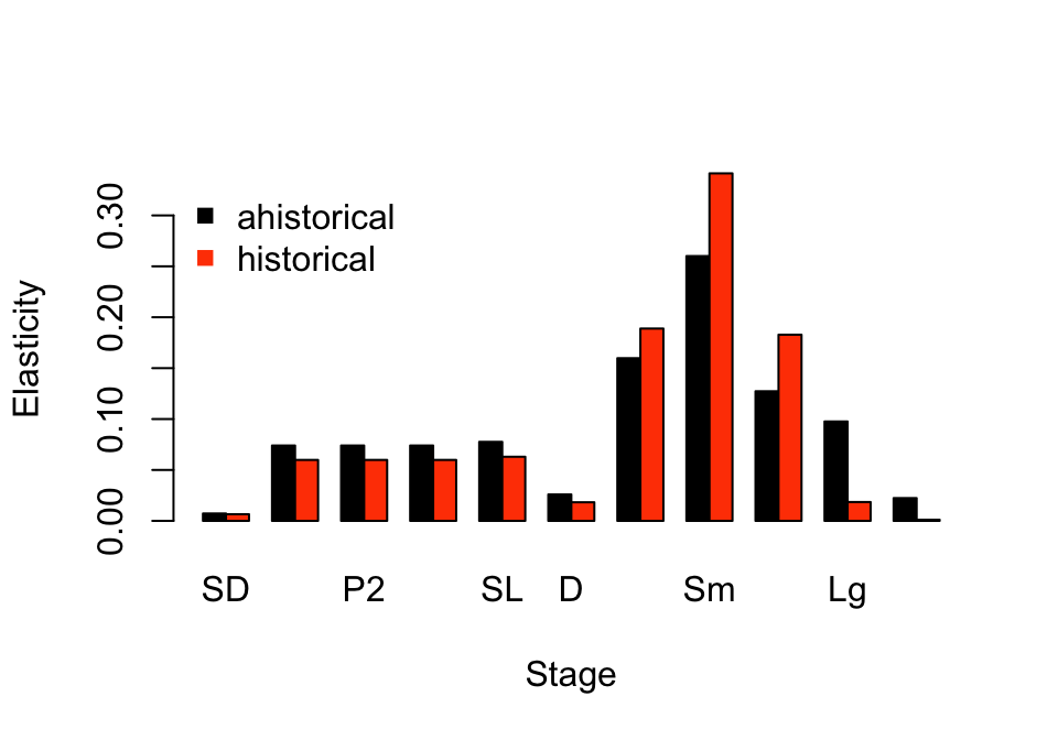
Figure 9.4: Ahistorical vs. historically-corrected deterministic elasticity to stage
Elasticity patterns in the two analyses look somewhat different. Both ahistorical and historical analyses show that \(\lambda\) is most elastic to shifts in transitions from the small adult stage, followed by the extra small and medium adult stages. However, historical analysis suggests a far greater importance to the small adult stage, and generally lower importance to juvenile stages and to large and extra large adults. So, once again, we see an important impact of individual history here.
Finally, let’s look at the elasticity sums of different transition types (figure 9.5).
tm2elas_r_sums <- summary(tm2elas_r)
tm3elas_r_sums <- summary(tm3elas_r)

elas_sums_together <- cbind.data.frame(tm2elas_r_sums$ahist[,2],
  tm3elas_r_sums$ahist[,2])
names(elas_sums_together) <- c("ahistorical", "historical")
rownames(elas_sums_together) <- tm2elas_r_sums$ahist$category

barplot(t(elas_sums_together), beside = T, ylab = "Elasticity",
  xlab = "Transition", col = c("black", "orangered"), bty = "n")
legend("topright", c("ahistorical", "historical"),
  col = c("black", "orangered"), pch = 15, bty = "n")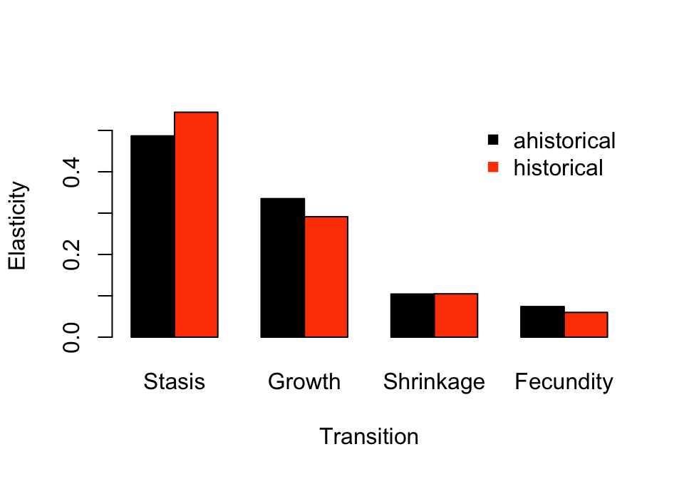
Figure 9.5: Ahistorical vs. historically-corrected elasticity to transitions
Fecundity has the least impact in both cases, although it does influence ahistorical analysis a reasonable amount. Stasis, in contrast, exerts the greatest influence, while growth is more influential than shrinkage and fecundity. We can also look at historical transitions, as below (figure 9.6).
elas_hist2plot <- as.matrix(tm3elas_r_sums$hist[,2])
rownames(elas_hist2plot) <- tm3elas_r_sums$hist$category

par(mar = c(7, 4, 2, 2) + 0.2)
barplot(t(elas_hist2plot), ylab = "Elasticity", xlab = "", xaxt = "n",
  col = "orangered", bty = "n")
text(cex=0.6, x=seq(from = -0.3, to = 1.15*length(tm3elas_r_sums$hist$category),
    by = 1.17), y=-0.08, tm3elas_r_sums$hist$category, xpd=TRUE, srt=45)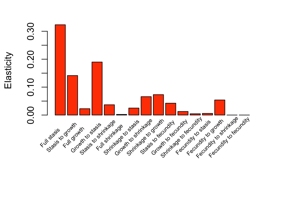
Figure 9.6: Elasticity of lambda to historical transitions
We can see that full stasis (i.e. staying in the same stage from occasion t-1 to t+1) is associated with the greatest summed elasticity values, and growth from occasion t-1 to t followed by stasis to occasion t+1 is the next most important. Transitions associated with fecundity are associated with the lowest summed elasticity values, except for fecundity followed by growth.
9.5 Analysis with bootstrapped MPMs
All of the functions described in this chapter work as easily with MPMs (class lefkoMat) as with lists of bootstrapped MPMs (class lefkoMatList). Let’s see by creating some bootstrapped empirical ahMPMs for Cypripedium candidum, and then trying out some analyses. First, we create the bootstrapped MPMs.
set.seed(42)
cypraw_v1_boot <- bootstrap3(cypraw_v1, reps = 3)

cypmatrix2r_boot <- rlefko2(data = cypraw_v1_boot, stageframe = cypframe_raw,
  year = "all", stages = c("stage3", "stage2"),
  size = c("size3added", "size2added"), supplement = cypsupp2_raw,
  yearcol = "year2", indivcol = "individ")

summary(cypmatrix2r_boot)
>
> This lefkoMatList object contains 3 ahistorical lefkoMat objects.
> The average lefkoMat object contains 5 matrices.
>
> This lefkoMatList object covers an average of 1 population, 1 patch, and 5 time steps.
> Each matrix is square with 11 rows and columns, and a total of 121 elements.
> An average of 106.667 survival transitions were estimated in each lefkoMat object,
> with an average of 21.333 per matrix.
> An average of 32 fecundity transitions were estimated in each lefkoMat object,
> with an average of 6.4 per matrix.
>
> The datasets contain an average total of 48 unique individuals and 304 unique transitions.
Since we are conducting deterministic analyses, we will create arithmetic mean matrices for each bootstrap, as below.
cyp2r_mean_boot <- lmean(cypmatrix2r_boot)

summary(cyp2r_mean_boot)
>
> This lefkoMatList object contains 3 ahistorical lefkoMat objects.
> The average lefkoMat object contains 1 matrix.
>
> This lefkoMatList object covers an average of 1 population, 1 patch, and 0 time steps.
> Each matrix is square with 11 rows and columns, and a total of 121 elements.
> An average of 31 survival transitions were estimated in each lefkoMat object,
> with an average of 31 per matrix.
> An average of 8.667 fecundity transitions were estimated in each lefkoMat object,
> with an average of 8.667 per matrix.
>
> The datasets contain an average total of 48 unique individuals and 304 unique transitions.
Now, let’s try finding the asymptotic population growth rates of these mean matrices.
We can continue on to find the associated stable stage distributions and reproductive value vectors. Let’s try the stable stage distributions first.
stablestage3(cyp2r_mean_boot)
> $mean
>    matrix stage_id stage      ss_prop
> 1       1        1    SD 4.696824e-01
> 2       1        2    P1 4.787046e-01
> 3       1        3    P2 4.597765e-02
> 4       1        4    P3 4.417037e-03
> 5       1        5    SL 2.229353e-04
> 6       1        6  Dorm 5.298496e-05
> 7       1        7   XSm 3.738172e-04
> 8       1        8    Sm 3.802692e-04
> 9       1        9    Md 1.240934e-04
> 10      1       10    Lg 5.754191e-05
> 11      1       11   XLg 6.732890e-06
>
> $summaries
> $summaries[[1]]
>    matrix stage_id stage      ss_prop
> 1       1        1    SD 4.704501e-01
> 2       1        2    P1 4.792895e-01
> 3       1        3    P2 4.502720e-02
> 4       1        4    P3 4.230113e-03
> 5       1        5    SL 2.084941e-04
> 6       1        6  Dorm 4.982613e-05
> 7       1        7   XSm 2.782307e-04
> 8       1        8    Sm 2.813996e-04
> 9       1        9    Md 1.092064e-04
> 10      1       10    Lg 6.989707e-05
> 11      1       11   XLg 6.011215e-06
>
> $summaries[[2]]
>    matrix stage_id stage      ss_prop
> 1       1        1    SD 4.691911e-01
> 2       1        2    P1 4.783205e-01
> 3       1        3    P2 4.653540e-02
> 4       1        4    P3 4.527391e-03
> 5       1        5    SL 2.314940e-04
> 6       1        6  Dorm 4.922022e-05
> 7       1        7   XSm 4.847414e-04
> 8       1        8    Sm 4.721118e-04
> 9       1        9    Md 1.596497e-04
> 10      1       10    Lg 2.843059e-05
> 11      1       11   XLg 0.000000e+00
>
> $summaries[[3]]
>    matrix stage_id stage      ss_prop
> 1       1        1    SD 4.694060e-01
> 2       1        2    P1 4.785037e-01
> 3       1        3    P2 4.637033e-02
> 4       1        4    P3 4.493608e-03
> 5       1        5    SL 2.288179e-04
> 6       1        6  Dorm 5.990854e-05
> 7       1        7   XSm 3.584794e-04
> 8       1        8    Sm 3.872963e-04
> 9       1        9    Md 1.034243e-04
> 10      1       10    Lg 7.429807e-05
> 11      1       11   XLg 1.418746e-05
We can see that there is a structure to the output. The first data frame (element mean) gives the mean stable stage distribution across the bootstrap replicates. This is followed by each matrix in order corresponding to each bootstrap replicate (the summaries elements). Reproductive value vectors via function repvalue3() work in the same way.
Sensitivity and elasticity analysis result in the same structure as above, with a mean element giving the mean element values, followed by summaries elements corresponding to each bootstrapped MPM in order.
sensitivity3(cyp2r_mean_boot)
> Running deterministic analysis...
> Running deterministic analysis...
> Running deterministic analysis...
> $mean
> $h_sensmats
> NULL
>
> $ah_sensmats
> $ah_sensmats[[1]]
> [,1] [,2] [,3] [,4] [,5]
> [1,] 7.016187e-03 7.150814e-03 6.860544e-04 6.583726e-05 3.319176e-06
> [2,] 6.753653e-02 6.883206e-02 6.601971e-03 6.333846e-04 3.192288e-05
> [3,] 7.043200e-01 7.178273e-01 6.883206e-02 6.601971e-03 3.326537e-04
> [4,] 7.347070e+00 7.487934e+00 7.178273e-01 6.883206e-02 3.467312e-03
> [5,] 1.533211e+02 1.562600e+02 1.497587e+01 1.435655e+00 7.229937e-02
> [6,] 2.096772e+02 2.136870e+02 2.043238e+01 1.954233e+00 9.817781e-02
> [7,] 2.280623e+02 2.324335e+02 2.227465e+01 2.135189e+00 1.075192e-01
> [8,] 3.434871e+02 3.500727e+02 3.355966e+01 3.218024e+00 1.621032e-01
> [9,] 5.084768e+02 5.182294e+02 4.969808e+01 4.767256e+00 2.402343e-01
> [10,] 7.986132e+02 8.139751e+02 7.828774e+01 7.531371e+00 3.806619e-01
> [11,] 5.674563e+02 5.783505e+02 5.551728e+01 5.330322e+00 2.688503e-01
> [,6] [,7] [,8] [,9] [,10]
> [1,] 7.888541e-07 5.514330e-06 5.607437e-06 1.843480e-06 8.678935e-07
> [2,] 7.588576e-06 5.289448e-05 5.378887e-05 1.771233e-05 8.380741e-06
> [3,] 7.909232e-05 5.498251e-04 5.591330e-04 1.844016e-04 8.765691e-05
> [4,] 8.245507e-04 5.716617e-03 5.813496e-03 1.920275e-03 9.170687e-04
> [5,] 1.719651e-02 1.189010e-01 1.209179e-01 4.000399e-02 1.919375e-02
> [6,] 2.355375e-02 1.562621e-01 1.595707e-01 5.310201e-02 2.755571e-02
> [7,] 2.565532e-02 1.759203e-01 1.792181e-01 5.909455e-02 2.888480e-02
> [8,] 3.862584e-02 2.665305e-01 2.713458e-01 8.941366e-02 4.316946e-02
> [9,] 5.718007e-02 3.968428e-01 4.038152e-01 1.329078e-01 6.346169e-02
> [10,] 9.040413e-02 6.463682e-01 6.575522e-01 2.128100e-01 9.636838e-02
> [11,] 6.861540e-02 4.031568e-01 4.284112e-01 1.270967e-01 8.811592e-02
> [,11]
> [1,] 9.975282e-08
> [2,] 9.602788e-07
> [3,] 1.001476e-05
> [4,] 1.044668e-04
> [5,] 2.179925e-03
> [6,] 3.186878e-03
> [7,] 3.344617e-03
> [8,] 4.981343e-03
> [9,] 7.313989e-03
> [10,] 1.147880e-02
> [11,] 1.409226e-02
>
>
> $hstages
> NULL
>
> $ahstages
> stage_id stage original_size original_size_b original_size_c min_age max_age
> 1 1 SD 0.0 NA NA 0 NA
> 2 2 P1 0.0 NA NA 0 NA
> 3 3 P2 0.0 NA NA 0 NA
> 4 4 P3 0.0 NA NA 0 NA
> 5 5 SL 0.0 NA NA 0 NA
> 6 6 Dorm 0.0 NA NA 0 NA
> 7 7 XSm 1.0 NA NA 0 NA
> 8 8 Sm 3.0 NA NA 0 NA
> 9 9 Md 6.0 NA NA 0 NA
> 10 10 Lg 11.0 NA NA 0 NA
> 11 11 XLg 19.5 NA NA 0 NA
> repstatus obsstatus propstatus immstatus matstatus entrystage indataset
> 1 0 0 1 0 0 1 0
> 2 0 0 0 1 0 1 0
> 3 0 0 0 1 0 0 0
> 4 0 0 0 1 0 0 0
> 5 0 0 0 1 0 0 0
> 6 0 0 0 0 1 0 1
> 7 1 1 0 0 1 0 1
> 8 1 1 0 0 1 0 1
> 9 1 1 0 0 1 0 1
> 10 1 1 0 0 1 0 1
> 11 1 1 0 0 1 0 1
> binhalfwidth_raw sizebin_min sizebin_max sizebin_center sizebin_width
> 1 0.0 0.0 0.0 0.0 0
> 2 0.0 0.0 0.0 0.0 0
> 3 0.0 0.0 0.0 0.0 0
> 4 0.0 0.0 0.0 0.0 0
> 5 0.0 0.0 0.0 0.0 0
> 6 0.5 -0.5 0.5 0.0 1
> 7 0.5 0.5 1.5 1.0 1
> 8 1.5 1.5 4.5 3.0 3
> 9 1.5 4.5 7.5 6.0 3
> 10 3.5 7.5 14.5 11.0 7
> 11 5.0 14.5 24.5 19.5 10
> binhalfwidthb_raw sizebinb_min sizebinb_max sizebinb_center sizebinb_width
> 1 NA NA NA NA NA
> 2 NA NA NA NA NA
> 3 NA NA NA NA NA
> 4 NA NA NA NA NA
> 5 NA NA NA NA NA
> 6 NA NA NA NA NA
> 7 NA NA NA NA NA
> 8 NA NA NA NA NA
> 9 NA NA NA NA NA
> 10 NA NA NA NA NA
> 11 NA NA NA NA NA
> binhalfwidthc_raw sizebinc_min sizebinc_max sizebinc_center sizebinc_width
> 1 NA NA NA NA NA
> 2 NA NA NA NA NA
> 3 NA NA NA NA NA
> 4 NA NA NA NA NA
> 5 NA NA NA NA NA
> 6 NA NA NA NA NA
> 7 NA NA NA NA NA
> 8 NA NA NA NA NA
> 9 NA NA NA NA NA
> 10 NA NA NA NA NA
> 11 NA NA NA NA NA
> group comments alive almostborn
> 1 0 Dormant seed 1 0
> 2 0 1st yr protocorm 1 0
> 3 0 2nd yr protocorm 1 0
> 4 0 3rd yr protocorm 1 0
> 5 0 Seedling 1 0
> 6 0 Dormant adult 1 0
> 7 0 Extra small adult (1 shoot) 1 0
> 8 0 Small adult (2-4 shoots) 1 0
> 9 0 Medium adult (5-7 shoots) 1 0
> 10 0 Large adult (8-14 shoots) 1 0
> 11 0 Extra large adult (>14 shoots) 1 0
>
> $agestages
> X1
> 1 NA
>
> $labels
> pop patch
> 1 1 1
>
> attr(,"class")
> [1] "lefkoSens"
>
> $summaries
> $summaries[[1]]
> $h_sensmats
> NULL
>
> $ah_sensmats
> $ah_sensmats[[1]]
> [,1] [,2] [,3] [,4] [,5]
> [1,] 7.733743e-03 7.879054e-03 7.402034e-04 6.953895e-05 3.427440e-06
> [2,] 7.613440e-02 7.756490e-02 7.286891e-03 6.845723e-04 3.374124e-05
> [3,] 8.104084e-01 8.256353e-01 7.756490e-02 7.286891e-03 3.591568e-04
> [4,] 8.626346e+00 8.788428e+00 8.256353e-01 7.756490e-02 3.823024e-03
> [5,] 1.836453e+02 1.870959e+02 1.757686e+01 1.651271e+00 8.138793e-02
> [6,] 2.924158e+02 2.979101e+02 2.798738e+01 2.629295e+00 1.295928e-01
> [7,] 2.734724e+02 2.786107e+02 2.617429e+01 2.458962e+00 1.211975e-01
> [8,] 4.020355e+02 4.095894e+02 3.847918e+01 3.614954e+00 1.781741e-01
> [9,] 5.791147e+02 5.899957e+02 5.542758e+01 5.207184e+00 2.566520e-01
> [10,] 6.989700e+02 7.121031e+02 6.689904e+01 6.284879e+00 3.097695e-01
> [11,] 5.259498e+02 5.358319e+02 5.033912e+01 4.729145e+00 2.330904e-01
> [,6] [,7] [,8] [,9] [,10]
> [1,] 8.190933e-07 4.573842e-06 4.625936e-06 1.795248e-06 1.149040e-06
> [2,] 8.063518e-06 4.502693e-05 4.553976e-05 1.767321e-05 1.131166e-05
> [3,] 8.583166e-05 4.792867e-04 4.847455e-04 1.881215e-04 1.204063e-04
> [4,] 9.136303e-04 5.101740e-03 5.159846e-03 2.002449e-03 1.281658e-03
> [5,] 1.945017e-02 1.086104e-01 1.098474e-01 4.262991e-02 2.728508e-02
> [6,] 3.097024e-02 1.729388e-01 1.749084e-01 6.787901e-02 4.344565e-02
> [7,] 2.896390e-02 1.617353e-01 1.635774e-01 6.348163e-02 4.063112e-02
> [8,] 4.258023e-02 2.377693e-01 2.404774e-01 9.332522e-02 5.973237e-02
> [9,] 6.133497e-02 3.424964e-01 3.463972e-01 1.344309e-01 8.604188e-02
> [10,] 7.402905e-02 4.133805e-01 4.180886e-01 1.622532e-01 1.038494e-01
> [11,] 5.570419e-02 3.110539e-01 3.145966e-01 1.220897e-01 7.814292e-02
> [,11]
> [1,] 9.881854e-08
> [2,] 9.728136e-07
> [3,] 1.035506e-05
> [4,] 1.102238e-04
> [5,] 2.346543e-03
> [6,] 3.736367e-03
> [7,] 3.494316e-03
> [8,] 5.137042e-03
> [9,] 7.399685e-03
> [10,] 8.931147e-03
> [11,] 6.720366e-03
>
>
> $hstages
> NULL
>
> $ahstages
> stage_id stage original_size original_size_b original_size_c min_age max_age
> 1 1 SD 0.0 NA NA 0 NA
> 2 2 P1 0.0 NA NA 0 NA
> 3 3 P2 0.0 NA NA 0 NA
> 4 4 P3 0.0 NA NA 0 NA
> 5 5 SL 0.0 NA NA 0 NA
> 6 6 Dorm 0.0 NA NA 0 NA
> 7 7 XSm 1.0 NA NA 0 NA
> 8 8 Sm 3.0 NA NA 0 NA
> 9 9 Md 6.0 NA NA 0 NA
> 10 10 Lg 11.0 NA NA 0 NA
> 11 11 XLg 19.5 NA NA 0 NA
> repstatus obsstatus propstatus immstatus matstatus entrystage indataset
> 1 0 0 1 0 0 1 0
> 2 0 0 0 1 0 1 0
> 3 0 0 0 1 0 0 0
> 4 0 0 0 1 0 0 0
> 5 0 0 0 1 0 0 0
> 6 0 0 0 0 1 0 1
> 7 1 1 0 0 1 0 1
> 8 1 1 0 0 1 0 1
> 9 1 1 0 0 1 0 1
> 10 1 1 0 0 1 0 1
> 11 1 1 0 0 1 0 1
> binhalfwidth_raw sizebin_min sizebin_max sizebin_center sizebin_width
> 1 0.0 0.0 0.0 0.0 0
> 2 0.0 0.0 0.0 0.0 0
> 3 0.0 0.0 0.0 0.0 0
> 4 0.0 0.0 0.0 0.0 0
> 5 0.0 0.0 0.0 0.0 0
> 6 0.5 -0.5 0.5 0.0 1
> 7 0.5 0.5 1.5 1.0 1
> 8 1.5 1.5 4.5 3.0 3
> 9 1.5 4.5 7.5 6.0 3
> 10 3.5 7.5 14.5 11.0 7
> 11 5.0 14.5 24.5 19.5 10
> binhalfwidthb_raw sizebinb_min sizebinb_max sizebinb_center sizebinb_width
> 1 NA NA NA NA NA
> 2 NA NA NA NA NA
> 3 NA NA NA NA NA
> 4 NA NA NA NA NA
> 5 NA NA NA NA NA
> 6 NA NA NA NA NA
> 7 NA NA NA NA NA
> 8 NA NA NA NA NA
> 9 NA NA NA NA NA
> 10 NA NA NA NA NA
> 11 NA NA NA NA NA
> binhalfwidthc_raw sizebinc_min sizebinc_max sizebinc_center sizebinc_width
> 1 NA NA NA NA NA
> 2 NA NA NA NA NA
> 3 NA NA NA NA NA
> 4 NA NA NA NA NA
> 5 NA NA NA NA NA
> 6 NA NA NA NA NA
> 7 NA NA NA NA NA
> 8 NA NA NA NA NA
> 9 NA NA NA NA NA
> 10 NA NA NA NA NA
> 11 NA NA NA NA NA
> group comments alive almostborn
> 1 0 Dormant seed 1 0
> 2 0 1st yr protocorm 1 0
> 3 0 2nd yr protocorm 1 0
> 4 0 3rd yr protocorm 1 0
> 5 0 Seedling 1 0
> 6 0 Dormant adult 1 0
> 7 0 Extra small adult (1 shoot) 1 0
> 8 0 Small adult (2-4 shoots) 1 0
> 9 0 Medium adult (5-7 shoots) 1 0
> 10 0 Large adult (8-14 shoots) 1 0
> 11 0 Extra large adult (>14 shoots) 1 0
>
> $agestages
> X1
> 1 NA
>
> $labels
> pop patch
> 1 1 1
>
> attr(,"class")
> [1] "lefkoSens"
>
> $summaries[[2]]
> $h_sensmats
> NULL
>
> $ah_sensmats
> $ah_sensmats[[1]]
> [,1] [,2] [,3] [,4] [,5]
> [1,] 6.683066e-03 6.813104e-03 6.628413e-04 6.448728e-05 3.297355e-06
> [2,] 6.334635e-02 6.457894e-02 6.282831e-03 6.112514e-04 3.125443e-05
> [3,] 6.511141e-01 6.637834e-01 6.457894e-02 6.282831e-03 3.212529e-04
> [4,] 6.692565e+00 6.822788e+00 6.637834e-01 6.457894e-02 3.302042e-03
> [5,] 1.375809e+02 1.402579e+02 1.364558e+01 1.327567e+00 6.788098e-02
> [6,] 1.439141e+02 1.467144e+02 1.427372e+01 1.388678e+00 7.100573e-02
> [7,] 1.943477e+02 1.981293e+02 1.927584e+01 1.875330e+00 9.588914e-02
> [8,] 3.039518e+02 3.098660e+02 3.014661e+01 2.932939e+00 1.499667e-01
> [9,] 4.651701e+02 4.742213e+02 4.613660e+01 4.488592e+00 2.295101e-01
> [10,] 8.530026e+02 8.696001e+02 8.460268e+01 8.230924e+00 4.208626e-01
> [11,] 0.000000e+00 0.000000e+00 0.000000e+00 0.000000e+00 0.000000e+00
> [,6] [,7] [,8] [,9] [,10] [,11]
> [1,] 7.010833e-07 6.904562e-06 6.724668e-06 2.274019e-06 4.049598e-07 0
> [2,] 6.645313e-06 6.544583e-05 6.374068e-05 2.155460e-05 3.838467e-06 0
> [3,] 6.830476e-05 6.726939e-04 6.551673e-04 2.215518e-04 3.945421e-05 0
> [4,] 7.020798e-04 6.914376e-03 6.734226e-03 2.277251e-03 4.055354e-04 0
> [5,] 1.443284e-02 1.421407e-01 1.384373e-01 4.681406e-02 8.336702e-03 0
> [6,] 1.509723e-02 1.486838e-01 1.448100e-01 4.896904e-02 8.720464e-03 0
> [7,] 2.038794e-02 2.007889e-01 1.955575e-01 6.612987e-02 1.177648e-02 0
> [8,] 3.188589e-02 3.140256e-01 3.058439e-01 1.034244e-01 1.841793e-02 0
> [9,] 4.879841e-02 4.805872e-01 4.680658e-01 1.582815e-01 2.818695e-02 0
> [10,] 8.948375e-02 8.812735e-01 8.583125e-01 2.902476e-01 5.168762e-02 0
> [11,] 0.000000e+00 0.000000e+00 0.000000e+00 0.000000e+00 0.000000e+00 0
>
>
> $hstages
> NULL
>
> $ahstages
> stage_id stage original_size original_size_b original_size_c min_age max_age
> 1 1 SD 0.0 NA NA 0 NA
> 2 2 P1 0.0 NA NA 0 NA
> 3 3 P2 0.0 NA NA 0 NA
> 4 4 P3 0.0 NA NA 0 NA
> 5 5 SL 0.0 NA NA 0 NA
> 6 6 Dorm 0.0 NA NA 0 NA
> 7 7 XSm 1.0 NA NA 0 NA
> 8 8 Sm 3.0 NA NA 0 NA
> 9 9 Md 6.0 NA NA 0 NA
> 10 10 Lg 11.0 NA NA 0 NA
> 11 11 XLg 19.5 NA NA 0 NA
> repstatus obsstatus propstatus immstatus matstatus entrystage indataset
> 1 0 0 1 0 0 1 0
> 2 0 0 0 1 0 1 0
> 3 0 0 0 1 0 0 0
> 4 0 0 0 1 0 0 0
> 5 0 0 0 1 0 0 0
> 6 0 0 0 0 1 0 1
> 7 1 1 0 0 1 0 1
> 8 1 1 0 0 1 0 1
> 9 1 1 0 0 1 0 1
> 10 1 1 0 0 1 0 1
> 11 1 1 0 0 1 0 1
> binhalfwidth_raw sizebin_min sizebin_max sizebin_center sizebin_width
> 1 0.0 0.0 0.0 0.0 0
> 2 0.0 0.0 0.0 0.0 0
> 3 0.0 0.0 0.0 0.0 0
> 4 0.0 0.0 0.0 0.0 0
> 5 0.0 0.0 0.0 0.0 0
> 6 0.5 -0.5 0.5 0.0 1
> 7 0.5 0.5 1.5 1.0 1
> 8 1.5 1.5 4.5 3.0 3
> 9 1.5 4.5 7.5 6.0 3
> 10 3.5 7.5 14.5 11.0 7
> 11 5.0 14.5 24.5 19.5 10
> binhalfwidthb_raw sizebinb_min sizebinb_max sizebinb_center sizebinb_width
> 1 NA NA NA NA NA
> 2 NA NA NA NA NA
> 3 NA NA NA NA NA
> 4 NA NA NA NA NA
> 5 NA NA NA NA NA
> 6 NA NA NA NA NA
> 7 NA NA NA NA NA
> 8 NA NA NA NA NA
> 9 NA NA NA NA NA
> 10 NA NA NA NA NA
> 11 NA NA NA NA NA
> binhalfwidthc_raw sizebinc_min sizebinc_max sizebinc_center sizebinc_width
> 1 NA NA NA NA NA
> 2 NA NA NA NA NA
> 3 NA NA NA NA NA
> 4 NA NA NA NA NA
> 5 NA NA NA NA NA
> 6 NA NA NA NA NA
> 7 NA NA NA NA NA
> 8 NA NA NA NA NA
> 9 NA NA NA NA NA
> 10 NA NA NA NA NA
> 11 NA NA NA NA NA
> group comments alive almostborn
> 1 0 Dormant seed 1 0
> 2 0 1st yr protocorm 1 0
> 3 0 2nd yr protocorm 1 0
> 4 0 3rd yr protocorm 1 0
> 5 0 Seedling 1 0
> 6 0 Dormant adult 1 0
> 7 0 Extra small adult (1 shoot) 1 0
> 8 0 Small adult (2-4 shoots) 1 0
> 9 0 Medium adult (5-7 shoots) 1 0
> 10 0 Large adult (8-14 shoots) 1 0
> 11 0 Extra large adult (>14 shoots) 1 0
>
> $agestages
> X1
> 1 NA
>
> $labels
> pop patch
> 1 1 1
>
> attr(,"class")
> [1] "lefkoSens"
>
> $summaries[[3]]
> $h_sensmats
> NULL
>
> $ah_sensmats
> $ah_sensmats[[1]]
> [,1] [,2] [,3] [,4] [,5]
> [1,] 6.631752e-03 6.760285e-03 6.551186e-04 6.348555e-05 3.232733e-06
> [2,] 6.312882e-02 6.435234e-02 6.236190e-03 6.043301e-04 3.077295e-05
> [3,] 6.514375e-01 6.640632e-01 6.435234e-02 6.236190e-03 3.175515e-04
> [4,] 6.722299e+00 6.852586e+00 6.640632e-01 6.435234e-02 3.276871e-03
> [5,] 1.387372e+02 1.414261e+02 1.370517e+01 1.328126e+00 6.762922e-02
> [6,] 1.927016e+02 1.964364e+02 1.903605e+01 1.844726e+00 9.393486e-02
> [7,] 2.163669e+02 2.205604e+02 2.137384e+01 2.071274e+00 1.054708e-01
> [8,] 3.244739e+02 3.307626e+02 3.205320e+01 3.106178e+00 1.581689e-01
> [9,] 4.811457e+02 4.904710e+02 4.753005e+01 4.605992e+00 2.345406e-01
> [10,] 8.438669e+02 8.602222e+02 8.336151e+01 8.078310e+00 4.113537e-01
> [11,] 1.176419e+03 1.199220e+03 1.162127e+02 1.126182e+01 5.734606e-01
> [,6] [,7] [,8] [,9] [,10]
> [1,] 8.463859e-07 5.064586e-06 5.471709e-06 1.461175e-06 1.049681e-06
> [2,] 8.056897e-06 4.821069e-05 5.208616e-05 1.390918e-05 9.992096e-06
> [3,] 8.314055e-05 4.974946e-04 5.374864e-04 1.435313e-04 1.031102e-04
> [4,] 8.579420e-04 5.133735e-03 5.546417e-03 1.481125e-03 1.064012e-03
> [5,] 1.770651e-02 1.059518e-01 1.144689e-01 3.056798e-02 2.195947e-02
> [6,] 2.459379e-02 1.471638e-01 1.589937e-01 4.245796e-02 3.050101e-02
> [7,] 2.761411e-02 1.652367e-01 1.785195e-01 4.767215e-02 3.424678e-02
> [8,] 4.141139e-02 2.477966e-01 2.677161e-01 7.149137e-02 5.135806e-02
> [9,] 6.140684e-02 3.674449e-01 3.969825e-01 1.060109e-01 7.615625e-02
> [10,] 1.076996e-01 6.444505e-01 6.962555e-01 1.859293e-01 1.335681e-01
> [11,] 1.501420e-01 8.984165e-01 9.706368e-01 2.592006e-01 1.862048e-01
> [,11]
> [1,] 2.004399e-07
> [2,] 1.908023e-06
> [3,] 1.968923e-05
> [4,] 2.031766e-04
> [5,] 4.193231e-03
> [6,] 5.824266e-03
> [7,] 6.539534e-03
> [8,] 9.806988e-03
> [9,] 1.454228e-02
> [10,] 2.550527e-02
> [11,] 3.555642e-02
>
>
> $hstages
> NULL
>
> $ahstages
> stage_id stage original_size original_size_b original_size_c min_age max_age
> 1 1 SD 0.0 NA NA 0 NA
> 2 2 P1 0.0 NA NA 0 NA
> 3 3 P2 0.0 NA NA 0 NA
> 4 4 P3 0.0 NA NA 0 NA
> 5 5 SL 0.0 NA NA 0 NA
> 6 6 Dorm 0.0 NA NA 0 NA
> 7 7 XSm 1.0 NA NA 0 NA
> 8 8 Sm 3.0 NA NA 0 NA
> 9 9 Md 6.0 NA NA 0 NA
> 10 10 Lg 11.0 NA NA 0 NA
> 11 11 XLg 19.5 NA NA 0 NA
> repstatus obsstatus propstatus immstatus matstatus entrystage indataset
> 1 0 0 1 0 0 1 0
> 2 0 0 0 1 0 1 0
> 3 0 0 0 1 0 0 0
> 4 0 0 0 1 0 0 0
> 5 0 0 0 1 0 0 0
> 6 0 0 0 0 1 0 1
> 7 1 1 0 0 1 0 1
> 8 1 1 0 0 1 0 1
> 9 1 1 0 0 1 0 1
> 10 1 1 0 0 1 0 1
> 11 1 1 0 0 1 0 1
> binhalfwidth_raw sizebin_min sizebin_max sizebin_center sizebin_width
> 1 0.0 0.0 0.0 0.0 0
> 2 0.0 0.0 0.0 0.0 0
> 3 0.0 0.0 0.0 0.0 0
> 4 0.0 0.0 0.0 0.0 0
> 5 0.0 0.0 0.0 0.0 0
> 6 0.5 -0.5 0.5 0.0 1
> 7 0.5 0.5 1.5 1.0 1
> 8 1.5 1.5 4.5 3.0 3
> 9 1.5 4.5 7.5 6.0 3
> 10 3.5 7.5 14.5 11.0 7
> 11 5.0 14.5 24.5 19.5 10
> binhalfwidthb_raw sizebinb_min sizebinb_max sizebinb_center sizebinb_width
> 1 NA NA NA NA NA
> 2 NA NA NA NA NA
> 3 NA NA NA NA NA
> 4 NA NA NA NA NA
> 5 NA NA NA NA NA
> 6 NA NA NA NA NA
> 7 NA NA NA NA NA
> 8 NA NA NA NA NA
> 9 NA NA NA NA NA
> 10 NA NA NA NA NA
> 11 NA NA NA NA NA
> binhalfwidthc_raw sizebinc_min sizebinc_max sizebinc_center sizebinc_width
> 1 NA NA NA NA NA
> 2 NA NA NA NA NA
> 3 NA NA NA NA NA
> 4 NA NA NA NA NA
> 5 NA NA NA NA NA
> 6 NA NA NA NA NA
> 7 NA NA NA NA NA
> 8 NA NA NA NA NA
> 9 NA NA NA NA NA
> 10 NA NA NA NA NA
> 11 NA NA NA NA NA
> group comments alive almostborn
> 1 0 Dormant seed 1 0
> 2 0 1st yr protocorm 1 0
> 3 0 2nd yr protocorm 1 0
> 4 0 3rd yr protocorm 1 0
> 5 0 Seedling 1 0
> 6 0 Dormant adult 1 0
> 7 0 Extra small adult (1 shoot) 1 0
> 8 0 Small adult (2-4 shoots) 1 0
> 9 0 Medium adult (5-7 shoots) 1 0
> 10 0 Large adult (8-14 shoots) 1 0
> 11 0 Extra large adult (>14 shoots) 1 0
>
> $agestages
> X1
> 1 NA
>
> $labels
> pop patch
> 1 1 1
>
> attr(,"class")
> [1] "lefkoSens"Voilà! Enjoy the bootstrapping!
9.6 Points to remember
- Deterministic analysis refers to matrix projection in which a single matrix is projected forward indefinitely. Its asymptotic properties yield values such as the stable stage structure and reproductive values of each stage, as well as the population growth rate under the stable structure.
- Package
lefko3can conduct all major deterministic analyses even for large numbers of massive matrices, such as historical IPMs and age-by-stage MPMs. This includes even sensitivity and elasticity analyses.
- A simple means of assessing the influence of history on population dynamics is through the comparison of ahistorical projection analyses to the equivalent historically-corrected analyses, since the latter interprets the results of historical analyses but framed within the stageframe and matrix dimensions of the former.
- All deterministic analysis functions can be applied to bootstrapped MPMs of class
lefkoMatList.