Chapter 13 Special Analyses II: Quasi-Extinction Analysis
A learning experience is one of those things that says, ‘You know that thing you just did? Don’t do that.’
Conservation managers often need to conduct population viability analyses (PVAs), which are demographic projection studies designed to assess the persistence potential of a target population (Beissinger & Westphal 1998). The populations targeted are typically rare and potentially endangered organisms. A quasi-extinction analysis is a type of PVA in which a population is split into control and treatment groups, and both groups are projected with temporal stochasticity. The persistence of the populations across replicates is then compared. This comparison is meant to overcome the limitations of predicting extinction itself, which is notoriously difficult. Instead, quasi-extinction analyses produce relative extinction probabilities, usually expressed as ratios of the proportion of extinct treatment replicates to the proportion of extinct control replicates.
In the simplest type of quasi-extinction analysis, we might have demographic data for a full population that has not been treated experimentally. Alternatively, we might have a population in which some portion of the population has been treated differently than the rest for some number of years, with demographic data collected from both treatment and control groups. In the former case, we might parameterize control and treatment sets of MPMs that use different underlying assumptions. For example, we might assume in the treatment group that we have boosted the pollination rate, or we have increased the survival of established adults via increased surveillance and the use of fences. In the latter case, we have data that stems from the treatment and so do not need to make any different assumptions, but simply parameterize two sets of models corresponding to the control and treatment groups.
Once the models are parameterized, we may project the matrices forward by some amount of time that we view as reasonable for management purposes. Depending on the agency and the conservation plan, this might be anywhere from 5 to 100 years. If we conduct these as stochastic projections replicated 100 or 1000 times, then we can compare the proportion of these replicates that go extinct in both cases. Since we do not know the true extinction rate, we instead estimate the quasi-extinction probabilities for both groups for the time window involved, and what is most meaningful is their ratio. For example, a treatment strategy that lowers the quasi-extinction probability by 20% might be worth incorporating into a management plan.
13.1 Cypripedium candidum example
Here we will set up a quasi-extinction analysis. We will use this analysis to assess whether hand pollination can decrease the extinction risk of an endangered perennial herb, Cypripedium candidum. Let’s utilize the function-based approach, using a life history model previously seen in earlier chapters (see section 5.2 in chapter 5). We’ll start off loading the data.
Next we’ll build the stageframe. Since we will split the population into two groups later, we will assume the same underlying biology and so the same life history model.
stagevector <- c("SD", "P1", "P2", "P3", "SL", "Dorm", "1V", "2V", "3V", "4V",
"5V", "6V", "7V", "8V", "9V", "10V", "11V", "12V", "13V", "14V", "15V", "16V",
"17V", "18V", "19V", "20V", "21V", "22V", "23V", "24V", "1F", "2F", "3F",
"4F", "5F", "6F", "7F", "8F", "9F", "10F", "11F", "12F", "13F", "14F", "15F",
"16F", "17F", "18F", "19F", "20F", "21F", "22F", "23F", "24F")
indataset <- c(0, 0, 0, 0, 0, rep(1, 49))
sizevector <- c(0, 0, 0, 0, 0, seq(from = 0, t = 24), seq(from = 1, to = 24))
repvector <- c(0, 0, 0, 0, 0, rep(0, 25), rep(1, 24))
obsvector <- c(0, 0, 0, 0, 0, 0, rep(1, 48))
matvector <- c(0, 0, 0, 0, 0, rep(1, 49))
immvector <- c(0, 1, 1, 1, 1, rep(0, 49))
propvector <- c(1, rep(0, 53))
comments <- c("Dormant seed", "Yr1 protocorm", "Yr2 protocorm", "Yr3 protocorm",
"Seedling", "Veg dorm", "Veg adult 1 stem", "Veg adult 2 stems",
"Veg adult 3 stems", "Veg adult 4 stems", "Veg adult 5 stems",
"Veg adult 6 stems", "Veg adult 7 stems", "Veg adult 8 stems",
"Veg adult 9 stems", "Veg adult 10 stems", "Veg adult 11 stems",
"Veg adult 12 stems", "Veg adult 13 stems", "Veg adult 14 stems",
"Veg adult 15 stems", "Veg adult 16 stems", "Veg adult 17 stems",
"Veg adult 18 stems", "Veg adult 19 stems", "Veg adult 20 stems",
"Veg adult 21 stems", "Veg adult 22 stems", "Veg adult 23 stems",
"Veg adult 24 stems", "Flo adult 1 stem", "Flo adult 2 stems",
"Flo adult 3 stems", "Flo adult 4 stems", "Flo adult 5 stems",
"Flo adult 6 stems", "Flo adult 7 stems", "Flo adult 8 stems",
"Flo adult 9 stems", "Flo adult 10 stems", "Flo adult 11 stems",
"Flo adult 12 stems", "Flo adult 13 stems", "Flo adult 14 stems",
"Flo adult 15 stems", "Flo adult 16 stems", "Flo adult 17 stems",
"Flo adult 18 stems", "Flo adult 19 stems", "Flo adult 20 stems",
"Flo adult 21 stems", "Flo adult 22 stems", "Flo adult 23 stems",
"Flo adult 24 stems")
cypframe_fb <- sf_create(sizes = sizevector, stagenames = stagevector,
repstatus = repvector, obsstatus = obsvector, matstatus = matvector,
propstatus = propvector, immstatus = immvector, indataset = indataset,
comments = comments)
cypframe_fb
> stage size size_b size_c min_age max_age repstatus obsstatus propstatus
> 1 SD 0 NA NA NA NA 0 0 1
> 2 P1 0 NA NA NA NA 0 0 0
> 3 P2 0 NA NA NA NA 0 0 0
> 4 P3 0 NA NA NA NA 0 0 0
> 5 SL 0 NA NA NA NA 0 0 0
> 6 Dorm 0 NA NA NA NA 0 0 0
> 7 1V 1 NA NA NA NA 0 1 0
> 8 2V 2 NA NA NA NA 0 1 0
> 9 3V 3 NA NA NA NA 0 1 0
> 10 4V 4 NA NA NA NA 0 1 0
> 11 5V 5 NA NA NA NA 0 1 0
> 12 6V 6 NA NA NA NA 0 1 0
> 13 7V 7 NA NA NA NA 0 1 0
> 14 8V 8 NA NA NA NA 0 1 0
> 15 9V 9 NA NA NA NA 0 1 0
> 16 10V 10 NA NA NA NA 0 1 0
> 17 11V 11 NA NA NA NA 0 1 0
> 18 12V 12 NA NA NA NA 0 1 0
> 19 13V 13 NA NA NA NA 0 1 0
> 20 14V 14 NA NA NA NA 0 1 0
> 21 15V 15 NA NA NA NA 0 1 0
> 22 16V 16 NA NA NA NA 0 1 0
> 23 17V 17 NA NA NA NA 0 1 0
> 24 18V 18 NA NA NA NA 0 1 0
> 25 19V 19 NA NA NA NA 0 1 0
> 26 20V 20 NA NA NA NA 0 1 0
> 27 21V 21 NA NA NA NA 0 1 0
> 28 22V 22 NA NA NA NA 0 1 0
> 29 23V 23 NA NA NA NA 0 1 0
> 30 24V 24 NA NA NA NA 0 1 0
> 31 1F 1 NA NA NA NA 1 1 0
> 32 2F 2 NA NA NA NA 1 1 0
> 33 3F 3 NA NA NA NA 1 1 0
> 34 4F 4 NA NA NA NA 1 1 0
> immstatus matstatus indataset binhalfwidth_raw sizebin_min sizebin_max
> 1 0 0 0 0.5 -0.5 0.5
> 2 1 0 0 0.5 -0.5 0.5
> 3 1 0 0 0.5 -0.5 0.5
> 4 1 0 0 0.5 -0.5 0.5
> 5 1 0 0 0.5 -0.5 0.5
> 6 0 1 1 0.5 -0.5 0.5
> 7 0 1 1 0.5 0.5 1.5
> 8 0 1 1 0.5 1.5 2.5
> 9 0 1 1 0.5 2.5 3.5
> 10 0 1 1 0.5 3.5 4.5
> 11 0 1 1 0.5 4.5 5.5
> 12 0 1 1 0.5 5.5 6.5
> 13 0 1 1 0.5 6.5 7.5
> 14 0 1 1 0.5 7.5 8.5
> 15 0 1 1 0.5 8.5 9.5
> 16 0 1 1 0.5 9.5 10.5
> 17 0 1 1 0.5 10.5 11.5
> 18 0 1 1 0.5 11.5 12.5
> 19 0 1 1 0.5 12.5 13.5
> 20 0 1 1 0.5 13.5 14.5
> 21 0 1 1 0.5 14.5 15.5
> 22 0 1 1 0.5 15.5 16.5
> 23 0 1 1 0.5 16.5 17.5
> 24 0 1 1 0.5 17.5 18.5
> 25 0 1 1 0.5 18.5 19.5
> 26 0 1 1 0.5 19.5 20.5
> 27 0 1 1 0.5 20.5 21.5
> 28 0 1 1 0.5 21.5 22.5
> 29 0 1 1 0.5 22.5 23.5
> 30 0 1 1 0.5 23.5 24.5
> 31 0 1 1 0.5 0.5 1.5
> 32 0 1 1 0.5 1.5 2.5
> 33 0 1 1 0.5 2.5 3.5
> 34 0 1 1 0.5 3.5 4.5
> sizebin_center sizebin_width binhalfwidthb_raw sizebinb_min sizebinb_max
> 1 0 1 NA NA NA
> 2 0 1 NA NA NA
> 3 0 1 NA NA NA
> 4 0 1 NA NA NA
> 5 0 1 NA NA NA
> 6 0 1 NA NA NA
> 7 1 1 NA NA NA
> 8 2 1 NA NA NA
> 9 3 1 NA NA NA
> 10 4 1 NA NA NA
> 11 5 1 NA NA NA
> 12 6 1 NA NA NA
> 13 7 1 NA NA NA
> 14 8 1 NA NA NA
> 15 9 1 NA NA NA
> 16 10 1 NA NA NA
> 17 11 1 NA NA NA
> 18 12 1 NA NA NA
> 19 13 1 NA NA NA
> 20 14 1 NA NA NA
> 21 15 1 NA NA NA
> 22 16 1 NA NA NA
> 23 17 1 NA NA NA
> 24 18 1 NA NA NA
> 25 19 1 NA NA NA
> 26 20 1 NA NA NA
> 27 21 1 NA NA NA
> 28 22 1 NA NA NA
> 29 23 1 NA NA NA
> 30 24 1 NA NA NA
> 31 1 1 NA NA NA
> 32 2 1 NA NA NA
> 33 3 1 NA NA NA
> 34 4 1 NA NA NA
> sizebinb_center sizebinb_width binhalfwidthc_raw sizebinc_min sizebinc_max
> 1 NA NA NA NA NA
> 2 NA NA NA NA NA
> 3 NA NA NA NA NA
> 4 NA NA NA NA NA
> 5 NA NA NA NA NA
> 6 NA NA NA NA NA
> 7 NA NA NA NA NA
> 8 NA NA NA NA NA
> 9 NA NA NA NA NA
> 10 NA NA NA NA NA
> 11 NA NA NA NA NA
> 12 NA NA NA NA NA
> 13 NA NA NA NA NA
> 14 NA NA NA NA NA
> 15 NA NA NA NA NA
> 16 NA NA NA NA NA
> 17 NA NA NA NA NA
> 18 NA NA NA NA NA
> 19 NA NA NA NA NA
> 20 NA NA NA NA NA
> 21 NA NA NA NA NA
> 22 NA NA NA NA NA
> 23 NA NA NA NA NA
> 24 NA NA NA NA NA
> 25 NA NA NA NA NA
> 26 NA NA NA NA NA
> 27 NA NA NA NA NA
> 28 NA NA NA NA NA
> 29 NA NA NA NA NA
> 30 NA NA NA NA NA
> 31 NA NA NA NA NA
> 32 NA NA NA NA NA
> 33 NA NA NA NA NA
> 34 NA NA NA NA NA
> sizebinc_center sizebinc_width group comments
> 1 NA NA 0 Dormant seed
> 2 NA NA 0 Yr1 protocorm
> 3 NA NA 0 Yr2 protocorm
> 4 NA NA 0 Yr3 protocorm
> 5 NA NA 0 Seedling
> 6 NA NA 0 Veg dorm
> 7 NA NA 0 Veg adult 1 stem
> 8 NA NA 0 Veg adult 2 stems
> 9 NA NA 0 Veg adult 3 stems
> 10 NA NA 0 Veg adult 4 stems
> 11 NA NA 0 Veg adult 5 stems
> 12 NA NA 0 Veg adult 6 stems
> 13 NA NA 0 Veg adult 7 stems
> 14 NA NA 0 Veg adult 8 stems
> 15 NA NA 0 Veg adult 9 stems
> 16 NA NA 0 Veg adult 10 stems
> 17 NA NA 0 Veg adult 11 stems
> 18 NA NA 0 Veg adult 12 stems
> 19 NA NA 0 Veg adult 13 stems
> 20 NA NA 0 Veg adult 14 stems
> 21 NA NA 0 Veg adult 15 stems
> 22 NA NA 0 Veg adult 16 stems
> 23 NA NA 0 Veg adult 17 stems
> 24 NA NA 0 Veg adult 18 stems
> 25 NA NA 0 Veg adult 19 stems
> 26 NA NA 0 Veg adult 20 stems
> 27 NA NA 0 Veg adult 21 stems
> 28 NA NA 0 Veg adult 22 stems
> 29 NA NA 0 Veg adult 23 stems
> 30 NA NA 0 Veg adult 24 stems
> 31 NA NA 0 Flo adult 1 stem
> 32 NA NA 0 Flo adult 2 stems
> 33 NA NA 0 Flo adult 3 stems
> 34 NA NA 0 Flo adult 4 stems
> [ reached 'max' / getOption("max.print") -- omitted 20 rows ]Continuing on, we’ll now standardize the dataset.
cypfb <- verticalize3(data = cypdata, noyears = 6, firstyear = 2004,
  patchidcol = "patch", individcol = "plantid", blocksize = 4,
  sizeacol = "Inf2.04", sizebcol = "Inf.04", sizeccol = "Veg.04",
  repstracol = "Inf.04", repstrbcol = "Inf2.04", fecacol = "Pod.04",
  stageassign = cypframe_fb, stagesize = "sizeadded", NAas0 = TRUE,
  age_offset = 4)

summary_hfv(cypfb)
>
> This hfv dataset contains 320 rows, 57 variables, 1 population,
> 3 patches, 74 individuals, and 5 time steps.
Next let’s explore the variables that we will build our vital rate models from.
hfv_qc(data = cypfb, vitalrates = c("surv", "obs", "size", "repst", "fec"),
  size = c("size3added", "size2added", "size1added"))
> Survival:
>
>   Data subset has 58 variables and 320 transitions.
>
>   Variable alive3 has 0 missing values.
>   Variable alive3 is a binomial variable.
>
>   Numbers of categories in data subset in possible random variables:
>   indiv id: 74   (singleton categories: 6)
>   year2: 5   (singleton categories: 0)
>
> Observation status:
>
>   Data subset has 58 variables and 303 transitions.
>
>   Variable obsstatus3 has 0 missing values.
>   Variable obsstatus3 is a binomial variable.
>
>   Numbers of categories in data subset in possible random variables:
>   indiv id: 70   (singleton categories: 6)
>   year2: 5   (singleton categories: 0)
>
> Primary size:
>
>   Data subset has 58 variables and 288 transitions.
>
>   Variable size3added has 0 missing values.
>   Variable size3added appears to be an integer variable.
>
>   Variable size3added is fully positive, lacking even 0s.
>
>   Overdispersion test:
>     Mean size3added is 3.653
>     The variance in size3added is 13.41
>     The probability of this dispersion level by chance assuming that
>     the true mean size3added = variance in size3added,
>     and an alternative hypothesis of overdispersion, is 3.721e-138
>     Variable size3added is significantly overdispersed.
>
>   Zero-inflation and truncation tests:
>     Mean lambda in size3added is 0.02592
>     The actual number of 0s in size3added is 0
>     The expected number of 0s in size3added under the null hypothesis is 7.465
>     The probability of this deviation in 0s from expectation by chance is 0.9964
>     Variable size3added is not significantly zero-inflated.
>
>     Variable size3added does not include 0s, suggesting that a zero-truncated distribution may be warranted.
>
>   Numbers of categories in data subset in possible random variables:
>   indiv id: 70   (singleton categories: 6)
>   year2: 5   (singleton categories: 0)
>
> Reproductive status:
>
>   Data subset has 58 variables and 288 transitions.
>
>   Variable repstatus3 has 0 missing values.
>   Variable repstatus3 is a binomial variable.
>
>   Numbers of categories in data subset in possible random variables:
>   indiv id: 70   (singleton categories: 6)
>   year2: 5   (singleton categories: 0)
>
> Fecundity:
>
>   Data subset has 58 variables and 118 transitions.
>
>   Variable feca2 has 0 missing values.
>   Variable feca2 appears to be an integer variable.
>
>   Variable feca2 is fully non-negative.
>
>   Overdispersion test:
>     Mean feca2 is 0.7881
>     The variance in feca2 is 1.536
>     The probability of this dispersion level by chance assuming that
>     the true mean feca2 = variance in feca2,
>     and an alternative hypothesis of overdispersion, is 0.1193
>     Dispersion level in feca2 matches expectation.
>
>   Zero-inflation and truncation tests:
>     Mean lambda in feca2 is 0.4547
>     The actual number of 0s in feca2 is 68
>     The expected number of 0s in feca2 under the null hypothesis is 53.65
>     The probability of this deviation in 0s from expectation by chance is 5.904e-06
>     Variable feca2 is significantly zero-inflated.
>
>   Numbers of categories in data subset in possible random variables:
>   indiv id: 51   (singleton categories: 21)
>   year2: 5   (singleton categories: 0)
We have described these models previously, and so encourage the reader to skip back to chapter 5 to read our interpretations.
Next let’s build the vital rate models. Note that we have not yet introduced any differences in the population. So, these models will be used for both treatment and control groups.
cypmodels2 <- modelsearch(cypfb, historical = FALSE, approach = "mixed",
  vitalrates = c("surv", "obs", "size", "repst", "fec"), sizedist = "negbin",
  size.trunc = TRUE, fecdist = "poisson", fec.zero = TRUE, suite = "full",
  size = c("size3added", "size2added", "size1added"), quiet = "partial")
>
> Developing global model of survival probability...
>
> Global model of survival probability developed. Proceeding with model dredge...
>
> Developing global model of observation probability...
>
> Global model of observation probability developed. Proceeding with model dredge...
>
> Developing global model of primary size...
>
> Global model of primary size developed. Proceeding with model dredge...
>
> Developing global model of reproduction probability...
>
> Global model of reproduction probability developed. Proceeding with model dredge...
>
> Developing global model of fecundity...
>
> Global model of fecundity developed. Proceeding with model dredge...
>
> Finished selecting best-fit models.

summary(cypmodels2)
> This LefkoMod object includes 5 linear models.
> Best-fit model criterion used: aicc&k
>
>
>
> Survival model:
> Generalized linear mixed model fit by maximum likelihood (Laplace
>   Approximation) [glmerMod]
>  Family: binomial  ( logit )
> Formula: alive3 ~ size2added + (1 | year2) + (1 | individ)
>    Data: surv.data
>       AIC       BIC    logLik -2*log(L)  df.resid
>  128.1324  143.2057  -60.0662  120.1324       316
> Random effects:
>  Groups  Name        Std.Dev.
>  individ (Intercept) 1.198379
>  year2   (Intercept) 0.008826
> Number of obs: 320, groups:  individ, 74; year2, 5
> Fixed Effects:
> (Intercept)   size2added
>      2.0352       0.6344
> optimizer (Nelder_Mead) convergence code: 0 (OK) ; 0 optimizer warnings; 1 lme4 warnings
>
>
>
> Observation model:
> Generalized linear mixed model fit by maximum likelihood (Laplace
>   Approximation) [glmerMod]
>  Family: binomial  ( logit )
> Formula: obsstatus3 ~ size2added + (1 | year2) + (1 | individ)
>    Data: obs.data
>       AIC       BIC    logLik -2*log(L)  df.resid
>  118.2567  133.1117  -55.1284  110.2567       299
> Random effects:
>  Groups  Name        Std.Dev.
>  individ (Intercept) 1.078e-05
>  year2   (Intercept) 8.776e-01
> Number of obs: 303, groups:  individ, 70; year2, 5
> Fixed Effects:
> (Intercept)   size2added
>      2.4904       0.3134
> optimizer (Nelder_Mead) convergence code: 0 (OK) ; 0 optimizer warnings; 1 lme4 warnings
>
>
>
> Size model:
> Formula:          size3added ~ (1 | year2) + (1 | individ)
> Data: size.data
>       AIC       BIC    logLik -2*log(L)  df.resid
> 1008.2764 1022.9282 -500.1382 1000.2764       284
> Random-effects (co)variances:
>
> Conditional model:
>  Groups  Name        Std.Dev.
>  year2   (Intercept) 0.1109
>  individ (Intercept) 1.0561
>
> Number of obs: 288 / Conditional model: year2, 5; individ, 70
>
> Dispersion parameter for truncated_nbinom2 family (): 1.99e+07
>
> Fixed Effects:
>
> Conditional model:
> (Intercept)
>      0.5761
>
>
>
> Secondary size model:
> [1] 1
>
>
>
> Tertiary size model:
> [1] 1
>
>
>
> Reproductive status model:
> Generalized linear mixed model fit by maximum likelihood (Laplace
>   Approximation) [glmerMod]
>  Family: binomial  ( logit )
> Formula: repstatus3 ~ repstatus2 + size2added + (1 | year2) + (1 | individ)
>    Data: repst.data
>       AIC       BIC    logLik -2*log(L)  df.resid
>  333.6176  351.9324 -161.8088  323.6176       283
> Random effects:
>  Groups  Name        Std.Dev.
>  individ (Intercept) 0.1829
>  year2   (Intercept) 0.6250
> Number of obs: 288, groups:  individ, 70; year2, 5
> Fixed Effects:
> (Intercept)   repstatus2   size2added
>     -1.4631       1.6457       0.1715
>
>
>
> Fecundity model:
> Formula:          feca2 ~ size2added + (1 | year2) + (1 | individ)
> Zero inflation:         ~size2added + (1 | year2) + (1 | individ)
> Data: fec.data
>       AIC       BIC    logLik -2*log(L)  df.resid
>  248.8609  271.0264 -116.4305  232.8609       110
> Random-effects (co)variances:
>
> Conditional model:
>  Groups  Name        Std.Dev.
>  year2   (Intercept) 0.5760
>  individ (Intercept) 0.1639
>
> Zero-inflation model:
>  Groups  Name        Std.Dev.
>  year2   (Intercept) 1.642e-06
>  individ (Intercept) 3.089e-04
>
> Number of obs: 118 / Conditional model: year2, 5; individ, 51 / Zero-inflation model: year2, 5; individ, 51
>
> Fixed Effects:
>
> Conditional model:
> (Intercept)   size2added
>    -0.54014      0.06174
>
> Zero-inflation model:
> (Intercept)   size2added
>       3.865       -1.574
>
>
> Juvenile survival model:
> [1] 1
>
>
>
> Juvenile observation model:
> [1] 1
>
>
>
> Juvenile size model:
> [1] 1
>
>
>
> Juvenile secondary size model:
> [1] 1
>
>
>
> Juvenile tertiary size model:
> [1] 1
>
>
>
> Juvenile reproduction model:
> [1] 1
>
>
>
> Juvenile maturity model:
> [1] 1
>
>
>
>
>
> Number of models in survival table: 5
>
> Number of models in observation table: 5
>
> Number of models in size table: 5
>
> Number of models in secondary size table: 1
>
> Number of models in tertiary size table: 1
>
> Number of models in reproduction status table: 5
>
> Number of models in fecundity table: 25
>
> Number of models in juvenile survival table: 1
>
> Number of models in juvenile observation table: 1
>
> Number of models in juvenile size table: 1
>
> Number of models in juvenile secondary size table: 1
>
> Number of models in juvenile tertiary size table: 1
>
> Number of models in juvenile reproduction table: 1
>
> Number of models in juvenile maturity table: 1
>
>
>
>
>
> General model parameter names (column 1), and
> specific names used in these models (column 2):
>                       parameter_names mainparams
> 1                              time t      year2
> 2                          individual    individ
> 3                               patch      patch
> 4                   alive in time t+1      surv3
> 5                observed in time t+1       obs3
> 6                   sizea in time t+1      size3
> 7                   sizeb in time t+1     sizeb3
> 8                   sizec in time t+1     sizec3
> 9     reproductive status in time t+1     repst3
> 10              fecundity in time t+1       fec3
> 11                fecundity in time t       fec2
> 12                    sizea in time t      size2
> 13                  sizea in time t-1      size1
> 14                    sizeb in time t     sizeb2
> 15                  sizeb in time t-1     sizeb1
> 16                    sizec in time t     sizec2
> 17                  sizec in time t-1     sizec1
> 18      reproductive status in time t     repst2
> 19    reproductive status in time t-1     repst1
> 20        maturity status in time t+1     matst3
> 21          maturity status in time t     matst2
> 22                      age in time t        age
> 23                  density in time t    density
> 24   individual covariate a in time t   indcova2
> 25 individual covariate a in time t-1   indcova1
> 26   individual covariate b in time t   indcovb2
> 27 individual covariate b in time t-1   indcovb1
> 28   individual covariate c in time t   indcovc2
> 29 individual covariate c in time t-1   indcovc1
> 30              stage group in time t     group2
> 31            stage group in time t-1     group1
> 32       annual covariate a in time t  annucova2
> 33     annual covariate a in time t-1  annucova1
> 34       annual covariate b in time t  annucovb2
> 35     annual covariate b in time t-1  annucovb1
> 36       annual covariate c in time t  annucovc2
> 37     annual covariate c in time t-1  annucovc1
>
>
>
>
>
> Quality control:
>
> Survival model estimated with 74 individuals and 320 individual transitions.
> Survival model accuracy is 0.947.
> Observation status model estimated with 70 individuals and 303 individual transitions.
> Observation status model accuracy is 0.95.
> Primary size model estimated with 70 individuals and 288 individual transitions.
> Primary size model R-squared is 0.822.
> Secondary size model not estimated.
> Tertiary size model not estimated.
> Reproductive status model estimated with 70 individuals and 288 individual transitions.
> Reproductive status model accuracy is 0.715.
> Fecundity model estimated with 51 individuals and 118 individual transitions.
> Fecundity model R-squared is 0.562.
> Juvenile survival model not estimated.
> Juvenile observation status model not estimated.
> Juvenile primary size model not estimated.
> Juvenile secondary size model not estimated.
> Juvenile tertiary size model not estimated.
> Juvenile reproductive status model not estimated.
> Juvenile maturity status model not estimated.
Now we will finally introduce some differences in the population. Here, we will build two supplement tables, one for the control and one for the treatment group. We will assume that our treatment group is a hand-pollination treatment, in which volunteers will go into the population and pollinate these plants. Our preliminary data suggests that we might be able to triple the fruiting rate from 16% to 48% using this approach.
First the control supplement.
seeds_per_fruit <- 15000 # Mean number of seeds per fruit
germ_c <- 0.15
sl_mult <- 0.7 # Survival to 1st year

cypsupp2_control <- supplemental(stage3 = c("SD", "P1", "P2", "P3", "SL", "SL",
    "Dorm", "1V", "2V", "3V", "SD", "P1"),
  stage2 = c("SD", "SD", "P1", "P2", "P3", "SL", "SL", "SL", "SL", "SL", "rep",
    "rep"),
  eststage3 = c(NA, NA, NA, NA, NA, NA, "Dorm", "1V", "2V", "3V", NA, NA),
  eststage2 = c(NA, NA, NA, NA, NA, NA, "Dorm", "Dorm", "Dorm", "Dorm", NA, NA),
  givenrate = c(0.08, 0.1, 0.1, 0.1, 0.05, 0.05, NA, NA, NA, NA, NA, NA),
  multiplier = c(NA, NA, NA, NA, NA, NA, sl_mult, sl_mult, sl_mult, sl_mult,
    0.5 * seeds_per_fruit * germ_c, 0.5 * seeds_per_fruit * germ_c),
  type = c("S", "S", "S", "S", "S", "S", "S", "S", "S", "S", "R", "R"),
  stageframe = cypframe_fb, historical = FALSE)
> Warning: NA values in argument multiplier will be treated as 1 values.

cypsupp2_control
>    stage3 stage2 stage1 age2 eststage3 eststage2 eststage1 estage2 givenrate
> 1      SD     SD   <NA>   NA      <NA>      <NA>      <NA>      NA      0.08
> 2      P1     SD   <NA>   NA      <NA>      <NA>      <NA>      NA      0.10
> 3      P2     P1   <NA>   NA      <NA>      <NA>      <NA>      NA      0.10
> 4      P3     P2   <NA>   NA      <NA>      <NA>      <NA>      NA      0.10
> 5      SL     P3   <NA>   NA      <NA>      <NA>      <NA>      NA      0.05
> 6      SL     SL   <NA>   NA      <NA>      <NA>      <NA>      NA      0.05
> 7    Dorm     SL   <NA>   NA      Dorm      Dorm      <NA>      NA        NA
> 8      1V     SL   <NA>   NA        1V      Dorm      <NA>      NA        NA
> 9      2V     SL   <NA>   NA        2V      Dorm      <NA>      NA        NA
> 10     3V     SL   <NA>   NA        3V      Dorm      <NA>      NA        NA
> 11     SD    rep   <NA>   NA      <NA>      <NA>      <NA>      NA        NA
> 12     P1    rep   <NA>   NA      <NA>      <NA>      <NA>      NA        NA
>    offset multiplier convtype convtype_t12
> 1      NA        1.0        1            1
> 2      NA        1.0        1            1
> 3      NA        1.0        1            1
> 4      NA        1.0        1            1
> 5      NA        1.0        1            1
> 6      NA        1.0        1            1
> 7      NA        0.7        1            1
> 8      NA        0.7        1            1
> 9      NA        0.7        1            1
> 10     NA        0.7        1            1
> 11     NA     1125.0        3            1
> 12     NA     1125.0        3            1
Now the treatment supplement.
germ_t <- 0.48

cypsupp2_trt <- supplemental(stage3 = c("SD", "P1", "P2", "P3", "SL", "SL",
    "Dorm", "1V", "2V", "3V", "SD", "P1"),
  stage2 = c("SD", "SD", "P1", "P2", "P3", "SL", "SL", "SL", "SL", "SL", "rep",
    "rep"),
  eststage3 = c(NA, NA, NA, NA, NA, NA, "Dorm", "1V", "2V", "3V", NA, NA),
  eststage2 = c(NA, NA, NA, NA, NA, NA, "Dorm", "Dorm", "Dorm", "Dorm", NA, NA),
  givenrate = c(0.08, 0.1, 0.1, 0.1, 0.05, 0.05, NA, NA, NA, NA, NA, NA),
  multiplier = c(NA, NA, NA, NA, NA, NA, sl_mult, sl_mult, sl_mult, sl_mult,
    0.5 * seeds_per_fruit * germ_t, 0.5 * seeds_per_fruit * germ_t),
  type = c("S", "S", "S", "S", "S", "S", "S", "S", "S", "S", "R", "R"),
  stageframe = cypframe_fb, historical = FALSE)
> Warning: NA values in argument multiplier will be treated as 1 values.

cypsupp2_trt
>    stage3 stage2 stage1 age2 eststage3 eststage2 eststage1 estage2 givenrate
> 1      SD     SD   <NA>   NA      <NA>      <NA>      <NA>      NA      0.08
> 2      P1     SD   <NA>   NA      <NA>      <NA>      <NA>      NA      0.10
> 3      P2     P1   <NA>   NA      <NA>      <NA>      <NA>      NA      0.10
> 4      P3     P2   <NA>   NA      <NA>      <NA>      <NA>      NA      0.10
> 5      SL     P3   <NA>   NA      <NA>      <NA>      <NA>      NA      0.05
> 6      SL     SL   <NA>   NA      <NA>      <NA>      <NA>      NA      0.05
> 7    Dorm     SL   <NA>   NA      Dorm      Dorm      <NA>      NA        NA
> 8      1V     SL   <NA>   NA        1V      Dorm      <NA>      NA        NA
> 9      2V     SL   <NA>   NA        2V      Dorm      <NA>      NA        NA
> 10     3V     SL   <NA>   NA        3V      Dorm      <NA>      NA        NA
> 11     SD    rep   <NA>   NA      <NA>      <NA>      <NA>      NA        NA
> 12     P1    rep   <NA>   NA      <NA>      <NA>      <NA>      NA        NA
>    offset multiplier convtype convtype_t12
> 1      NA        1.0        1            1
> 2      NA        1.0        1            1
> 3      NA        1.0        1            1
> 4      NA        1.0        1            1
> 5      NA        1.0        1            1
> 6      NA        1.0        1            1
> 7      NA        0.7        1            1
> 8      NA        0.7        1            1
> 9      NA        0.7        1            1
> 10     NA        0.7        1            1
> 11     NA     3600.0        3            1
> 12     NA     3600.0        3            1
Finally, let’s run two simulations. We are interested in developing a management plant that will allow persistence for at least 10 years. So, let’s try a replicated stochastic simulation projecting 10 time steps forward.
First the control.
set.seed(42)

trial2f_control <- f_projection3(data = cypfb, format = 3, stochastic = TRUE,
  substoch = 2, stageframe = cypframe_fb, supplement = cypsupp2_control,
  modelsuite = cypmodels2, times = 10, nreps = 1000, integeronly = TRUE)
> Warning: Option patch not set, so will set to first patch/population.

summary(trial2f_control, ext_time = TRUE)
>
> The input lefkoProj object covers 1 population-patches.
> It is a single projection including 10 projected steps per replicate, and 1000 replicates, respectively.
> The number of replicates with population size above the threshold size of 1 is as in
> the following matrix, with pop-patches given by column and milepost times given by row:
> $milepost_sums
>       1 1
> 0    1000
> 0.25 1000
> 0.5  1000
> 0.75 1000
> 1     167
>
> $extinction_times
>   ext_reps ext_time
> 1      833  10.2473
Next the treatment simulation.
set.seed(42)

trial2f_trt <- f_projection3(data = cypfb, format = 3, stochastic = TRUE,
  substoch = 2, stageframe = cypframe_fb, supplement = cypsupp2_trt,
  modelsuite = cypmodels2, times = 10, nreps = 1000, integeronly = TRUE)
> Warning: Option patch not set, so will set to first patch/population.

summary(trial2f_trt, ext_time = TRUE)
>
> The input lefkoProj object covers 1 population-patches.
> It is a single projection including 10 projected steps per replicate, and 1000 replicates, respectively.
> The number of replicates with population size above the threshold size of 1 is as in
> the following matrix, with pop-patches given by column and milepost times given by row:
> $milepost_sums
>       1 1
> 0    1000
> 0.25 1000
> 0.5  1000
> 0.75 1000
> 1     983
>
> $extinction_times
>   ext_reps ext_time
> 1       17       11
The summaries all suggest that the hand pollination treatment leads to increased persistence. Let’s plot the results (13.1).
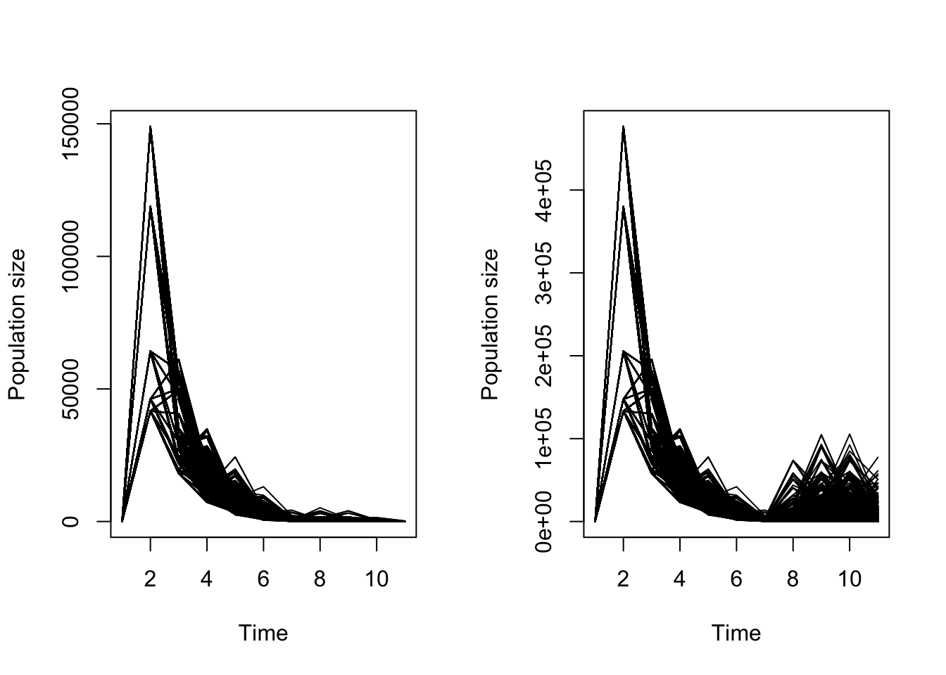
Figure 13.1: Quasi-extinction analysis. a) Control projection. b) Treatment projection with hand pollination
This certainly looks a lot better, particularly because of the difference in y-axis scale and the fact that many more replicates appear to survive in the treatment projections. But these plots are also perhaps a bit difficult to interpret. Our quasi-extinction analysis needs a bit more than this - a numeric metric showing us the difference in extinction probability. Let’s estimate the quasi-extinction probabilities.
control_sum <- summary(trial2f_control)
>
> The input lefkoProj object covers 1 population-patches.
> It is a single projection including 10 projected steps per replicate, and 1000 replicates, respectively.
> The number of replicates with population size above the threshold size of 1 is as in
> the following matrix, with pop-patches given by column and milepost times given by row:
trt_sum <- summary(trial2f_trt)
>
> The input lefkoProj object covers 1 population-patches.
> It is a single projection including 10 projected steps per replicate, and 1000 replicates, respectively.
> The number of replicates with population size above the threshold size of 1 is as in
> the following matrix, with pop-patches given by column and milepost times given by row:

control_ext <- 1 - (control_sum$milepost_sums[5] / control_sum$milepost_sums[1])
trt_ext <- 1 - (trt_sum$milepost_sums[5] / trt_sum$milepost_sums[1])

writeLines(paste("Control quasi-extinction prob: ", control_ext))
> Control quasi-extinction prob:  0.833
writeLines(paste("Treatment quasi-extinction prob: ", trt_ext))
> Treatment quasi-extinction prob:  0.017
Finally, let’s estimate the quasi-extinction ratio. This is the extinction probability of the treatment relative to the control.
And so we see that our hand pollination treatment reduces the chance of extinction to only 2% of the control over the next 10 years. This would suggest that our management plan is probably worth putting into action.
Naturally, quasi-extinction analysis is not exact and strongly dependent on assumptions. It is also dependent on conditions staying as they are during the monitoring period. We can try other approaches, including adding density dependence, shifting climate, etc. We will leave that to the user to try.
13.2 Points to remember
- Population viability analyses (PVA) use projection analyses to assess the persistence of populations.
- Quasi-extinction analysis is used to assess the impact of a treatment on the chance of populatoon extinction, given a comparison to a control.
- Functions
projection3()andf_projection3()allow users the ability to run paired projections to estimate quasi-extinction rates.