Chapter 8 Population Projection I: Projection Simulations
Now that I know that the right time has come
My prediction will surely be true
Projection matrices are typically used in population ecology with the aim of prediction, or of understanding the typical demographic properties of a population. In a projection analysis, one or more matrices are multiplied by a starting vector of individual numbers in each stage, typically referred to as a population vector. A general equation showing the process of projection is shown below.
\[\begin{equation} \mathbf{n_t} = \mathbf{A_t A_{t-1} \cdots A_1 n_0} \tag{8.1} \end{equation}\]
Here, each \(\mathbf{A_i}\) represents the matrix to be used at time \(i\). The original population vector is \(\mathbf{n_0}\), and this object is a one-column vector with the same number of rows as there are columns (and rows) in the projection matrix or matrices. This projection can be any number of time steps forward, perhaps only a small number to see how a particular management regime might impact population dynamics in the immediate term, or perhaps a very large number to assess equilibrial states and long-term patterns, such as cycles, plateaus, or chaos.
Package lefko3 provides a series of functions that can be used to run projections. Some are functions for special cases, such as deterministic or stochastic projections (see chapters 9 and 10, respectively). In this chapter, we will describe two functions that may be used for all general cases. We will also describe some simple uses of these functions. Details on advanced use of these functions will be described in chapters 9, 10, and 11. At the very end of this chapter we also introduce some functions to help manage projection output.
8.1 General projection functions
Package lefko3 provides two functions for general projection: projection3() and f_projection3(). The former is used to project matrices that have already been developed and exist within lefkoMat objects. The latter is used to take vital rate models and build new function-based matrices for each time step.
Many kinds of projections are possible with these functions, including deterministic, ordered, cyclical, and stochastic, all with and without density dependence. Let’s turn to two specific kinds of analyses that we might use these functions for:
- Simple projections of a specific time length
- Ordered or cyclical projections of a specific time length
We will use the Cypripedium candidum dataset for examples for both functions.
8.1.1 Set up for projection3() examples
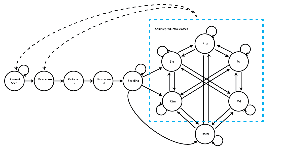
Function projection3() allows us to project existing matrices, contained within lefkoMat objects. Let’s set up our examples using the following life history model, which was originally introduced in chapter 3.
Here will build our raw Cypripedium MPMs.
data(cypdata)

sizevector <- c(0, 0, 0, 0, 0, 0, 1, 3, 6, 11, 19.5)
stagevector <- c("SD", "P1", "P2", "P3", "SL", "Dorm", "XSm", "Sm", "Md", "Lg",
  "XLg")
repvector <- c(0, 0, 0, 0, 0, 0, 1, 1, 1, 1, 1)
obsvector <- c(0, 0, 0, 0, 0, 0, 1, 1, 1, 1, 1)
matvector <- c(0, 0, 0, 0, 0, 1, 1, 1, 1, 1, 1)
immvector <- c(0, 1, 1, 1, 1, 0, 0, 0, 0, 0, 0)
propvector <- c(1, 0, 0, 0, 0, 0, 0, 0, 0, 0, 0)
indataset <- c(0, 0, 0, 0, 0, 1, 1, 1, 1, 1, 1)
binvec <- c(0, 0, 0, 0, 0, 0.5, 0.5, 1.5, 1.5, 3.5, 5)
comments <- c("Dormant seed", "1st yr protocorm", "2nd yr protocorm",
  "3rd yr protocorm", "Seedling", "Dormant adult",
  "Extra small adult (1 shoot)", "Small adult (2-4 shoots)",
  "Medium adult (5-7 shoots)", "Large adult (8-14 shoots)",
  "Extra large adult (>14 shoots)")
cypframe_raw <- sf_create(sizes = sizevector, stagenames = stagevector,
  repstatus = repvector, obsstatus = obsvector, matstatus = matvector,
  propstatus = propvector, immstatus = immvector, indataset = indataset,
  binhalfwidth = binvec, comments = comments)

cypraw_v1 <- verticalize3(data = cypdata, noyears = 6, firstyear = 2004,
  patchidcol = "patch", individcol = "plantid", blocksize = 4,
  sizeacol = "Inf2.04", sizebcol = "Inf.04", sizeccol = "Veg.04",
  repstracol = "Inf.04", repstrbcol = "Inf2.04", fecacol = "Pod.04",
  stageassign = cypframe_raw, stagesize = "sizeadded", NAas0 = TRUE,
  NRasRep = TRUE)

seeds_per_fruit <- 5000
sl_mult <- 0.7

cypsupp2_raw <- supplemental(stage3 = c("SD", "P1", "P2", "P3", "SL", "SL",
    "Dorm", "XSm", "Sm", "SD", "P1"),
  stage2= c("SD", "SD", "P1", "P2", "P3", "SL", "SL", "SL", "SL", "rep", "rep"),
  eststage3 = c(NA, NA, NA, NA, NA, NA, "Dorm", "XSm", "Sm", NA, NA),
  eststage2 = c(NA, NA, NA, NA, NA, NA, "XSm", "XSm", "XSm", NA, NA),
  givenrate = c(0.08, 0.10, 0.10, 0.10, 0.05, 0.05, NA, NA, NA, NA, NA),
  multiplier = c(NA, NA, NA, NA, NA, NA, sl_mult, sl_mult, sl_mult,
    0.5 * seeds_per_fruit, 0.5 * seeds_per_fruit),
  type =c(1, 1, 1, 1, 1, 1, 1, 1, 1, 3, 3),
  stageframe = cypframe_raw, historical = FALSE)
> Warning: NA values in argument multiplier will be treated as 1 values.

cypsupp3_raw <- supplemental(stage3 = c("SD", "SD", "P1", "P1", "P2", "P2",
    "P3", "SL", "SL", "SL", "Dorm", "XSm", "Sm", "Dorm", "XSm", "Sm", "mat",
    "mat", "mat", "SD", "P1"),
  stage2 = c("SD", "SD", "SD", "SD", "P1", "P1", "P2", "P3", "SL", "SL", "SL",
    "SL", "SL", "SL", "SL", "SL", "Dorm", "XSm", "Sm", "rep", "rep"),
  stage1 = c("SD", "rep", "SD", "rep", "SD", "rep", "P1", "P2", "P3", "SL",
    "SL", "SL", "SL", "P3", "P3", "P3", "SL", "SL", "SL", "mat", "mat"),
  eststage3 = c(NA, NA, NA, NA, NA, NA, NA, NA, NA, NA, "Dorm", "XSm", "Sm",
    "Dorm", "XSm", "Sm", "mat", "mat", "mat", NA, NA),
  eststage2 = c(NA, NA, NA, NA, NA, NA, NA, NA, NA, NA, "XSm", "XSm", "XSm",
    "XSm", "XSm", "XSm", "Dorm", "XSm", "Sm", NA, NA),
  eststage1 = c(NA, NA, NA, NA, NA, NA, NA, NA, NA, NA, "XSm", "XSm", "XSm",
    "XSm", "XSm", "XSm", "XSm", "XSm", "XSm", NA, NA),
  givenrate = c(0.08, 0.10, 0.10, 0.10, 0.10, 0.10, 0.10, 0.05, 0.05, 0.05, NA,
    NA, NA, NA, NA, NA, NA, NA, NA, NA, NA),
  multiplier = c(NA, NA, NA, NA, NA, NA, NA, NA, NA, NA, sl_mult, sl_mult,
    sl_mult, sl_mult, sl_mult, sl_mult, 1, 1, 1, 0.5 * seeds_per_fruit,
    0.5 * seeds_per_fruit),
  type =c(1, 1, 1, 1, 1, 1, 1, 1, 1, 1, 1, 1, 1, 1, 1, 1, 1, 1, 1, 3, 3),
  stageframe = cypframe_raw, historical = TRUE)
> Warning: NA values in argument multiplier will be treated as 1 values.

cypmatrix2r <- rlefko2(data = cypraw_v1, stageframe = cypframe_raw,
  year = "all", stages = c("stage3", "stage2"),
  size = c("size3added", "size2added"), supplement = cypsupp2_raw,
  yearcol = "year2", indivcol = "individ")

cypmatrix2rp <- rlefko2(data = cypraw_v1, stageframe = cypframe_raw,
  year = "all", patch = "all", stages = c("stage3", "stage2"),
  size = c("size3added", "size2added"), supplement = cypsupp2_raw,
  yearcol = "year2", patchcol = "patchid", indivcol = "individ")

cypmatrix3r <- rlefko3(data = cypraw_v1, stageframe = cypframe_raw,
  year = "all", stages = c("stage3", "stage2", "stage1"),
  size = c("size3added", "size2added", "size1added"), supplement = cypsupp3_raw,
  yearcol = "year2", indivcol = "individ", sparse_output = TRUE)

cypmatrix3rp <- rlefko3(data = cypraw_v1, stageframe = cypframe_raw,
  year = "all", patch = "all", stages = c("stage3", "stage2", "stage1"),
  size = c("size3added", "size2added", "size1added"), supplement = cypsupp3_raw,
  yearcol = "year2", patchcol = "patchid", indivcol = "individ",
  sparse_output = TRUE)
We have four MPMs. The first two, cypmatrix2r and cypmatrix2rp, are ahistorical MPMs at the population and patch level, respectively. The next two, cypmatrix3r and cypmatrix3rp, are historical MPMs at the population and patch level, respectively. Let’s see their summaries to jumpstart our memories about them.
summary(cypmatrix2r)
>
> This ahistorical lefkoMat object contains 5 matrices.
>
> Each matrix is square with 11 rows and columns, and a total of 121 elements.
> A total of 120 survival transitions were estimated, with 24 per matrix.
> A total of 40 fecundity transitions were estimated, with 8 per matrix.
> This lefkoMat object covers 1 population, 1 patch, and 5 time steps.
>
> The dataset contains a total of 74 unique individuals and 320 unique transitions.
>
> Survival probability sum check (each matrix represented by column in order):
>          [,1]  [,2]  [,3]  [,4]  [,5]
> Min.    0.000 0.050 0.050 0.000 0.050
> 1st Qu. 0.100 0.140 0.140 0.100 0.140
> Median  0.689 0.870 0.864 0.610 0.882
> Mean    0.552 0.629 0.629 0.528 0.627
> 3rd Qu. 1.000 1.000 1.000 0.960 1.000
> Max.    1.000 1.000 1.000 1.000 1.000
>
>
> Stages without connections leading to the rest of the life cycle found in matrices: 1 4

summary(cypmatrix2rp)
>
> This ahistorical lefkoMat object contains 15 matrices.
>
> Each matrix is square with 11 rows and columns, and a total of 121 elements.
> A total of 266 survival transitions were estimated, with 17.733 per matrix.
> A total of 70 fecundity transitions were estimated, with 4.667 per matrix.
> This lefkoMat object covers 1 population, 3 patches, and 5 time steps.
>
> The dataset contains a total of 74 unique individuals and 320 unique transitions.
>
> Survival probability sum check (each matrix represented by column in order):
>          [,1]  [,2]  [,3]  [,4]  [,5]  [,6]  [,7]  [,8]  [,9] [,10] [,11] [,12]
> Min.    0.000 0.000 0.000 0.000 0.000 0.000 0.050 0.050 0.000 0.050 0.000 0.000
> 1st Qu. 0.075 0.025 0.075 0.025 0.075 0.075 0.140 0.140 0.100 0.140 0.100 0.100
> Median  0.180 0.100 0.180 0.100 0.180 0.180 0.909 0.778 0.686 0.857 0.750 0.575
> Mean    0.457 0.361 0.471 0.328 0.417 0.464 0.631 0.611 0.530 0.631 0.562 0.523
> 3rd Qu. 0.955 0.769 1.000 0.592 0.781 1.000 1.000 1.000 0.955 1.000 1.000 1.000
> Max.    1.000 1.000 1.000 1.000 1.000 1.000 1.000 1.000 1.000 1.000 1.000 1.000
>         [,13] [,14] [,15]
> Min.    0.000 0.000 0.000
> 1st Qu. 0.075 0.075 0.100
> Median  0.180 0.180 0.750
> Mean    0.432 0.450 0.562
> 3rd Qu. 0.875 1.000 1.000
> Max.    1.000 1.000 1.000
>
>
> Stages without connections leading to the rest of the life cycle found in matrices: 1 2 3 4 5 6 9 11 12 13 14 15

summary(cypmatrix3r)
>
> This historical lefkoMat object contains 4 matrices.
>
> Each matrix is square with 121 rows and columns, and a total of 14641 elements.
> A total of 242 survival transitions were estimated, with 60.5 per matrix.
> A total of 54 fecundity transitions were estimated, with 13.5 per matrix.
> This lefkoMat object covers 1 population, 1 patch, and 4 time steps.
>
> The dataset contains a total of 74 unique individuals and 320 unique transitions.
>
> Survival probability sum check (each matrix represented by column in order):
>          [,1]  [,2]  [,3]  [,4]
> Min.    0.000 0.000 0.000 0.000
> 1st Qu. 0.000 0.000 0.000 0.000
> Median  0.000 0.000 0.000 0.000
> Mean    0.173 0.179 0.166 0.198
> 3rd Qu. 0.100 0.100 0.100 0.100
> Max.    1.000 1.000 1.000 1.000
>
>
> Stage-pairs without connections leading to them found in matrices: 1 2 3 4

summary(cypmatrix3rp)
>
> This historical lefkoMat object contains 12 matrices.
>
> Each matrix is square with 121 rows and columns, and a total of 14641 elements.
> A total of 516 survival transitions were estimated, with 43 per matrix.
> A total of 70 fecundity transitions were estimated, with 5.833 per matrix.
> This lefkoMat object covers 1 population, 3 patches, and 4 time steps.
>
> The dataset contains a total of 74 unique individuals and 320 unique transitions.
>
> Survival probability sum check (each matrix represented by column in order):
>          [,1]   [,2]   [,3]  [,4]  [,5]  [,6] [,7]  [,8]  [,9]  [,10] [,11]
> Min.    0.000 0.0000 0.0000 0.000 0.000 0.000 0.00 0.000 0.000 0.0000 0.000
> 1st Qu. 0.000 0.0000 0.0000 0.000 0.000 0.000 0.00 0.000 0.000 0.0000 0.000
> Median  0.000 0.0000 0.0000 0.000 0.000 0.000 0.00 0.000 0.000 0.0000 0.000
> Mean    0.107 0.0945 0.0851 0.101 0.158 0.158 0.14 0.169 0.119 0.0851 0.119
> 3rd Qu. 0.000 0.0000 0.0000 0.000 0.100 0.100 0.05 0.100 0.000 0.0000 0.000
> Max.    1.000 1.0000 1.0000 1.000 1.000 1.000 1.00 1.000 1.000 1.0000 1.000
>         [,12]
> Min.    0.000
> 1st Qu. 0.000
> Median  0.000
> Mean    0.144
> 3rd Qu. 0.000
> Max.    1.000
>
>
> Stage-pairs without connections leading to them found in matrices: 1 2 3 4 5 6 7 8 9 10 11 12
That’s essentially all of the core set-up for function projection3(). Now let’s move on to setting up the examples for f_projection3().
8.1.2 Set-up for f_projection3() examples
Function projection3() allows users to project matrices forward in time, but is limited to cases in which we have already developed MPMs and wish to project using only those matrices. What if we wished to create a new matrix at each time step, perhaps because changing conditions should alter basic vital rates at each time step? Function-based projection through function f_projection3() provides us with the flexibility to construct custom matrices at each time step given some set of conditions that we are interested in. The price paid is that it takes extra time to develop matrices at each time step in the projection, making standard MPM projection through function projection3() preferable except in cases where custom matrices are genuinely needed at each time step.
What sorts of situations might require custom matrices at each time step? One obvious situation is when matrices are to be built using set values of an individual or environmental covariate. For example, we may have developed a set of vital rate models that have relationships with climatic variables that are likely to change in the future. We might then wish to project the population forward under different climate change scenarios, with vectors of specific values of these climatic variables derived from climate prediction models (e.g., Shefferson et al. 2017). In this circumstance, using already made matrices in some sequence will not likely be of much help to us because matrices should change at each time step as a function of climate. Instead, we should create new matrices at each projected time, using values of the climatic variables that are relevant.
Let’s also explore this with the Cypripedium candidum dataset, as in the projection3() case. We introduced the model and code for for our stageframe and supplements in Chapter 2, and showed how to build function-based MPMs with all of this material in Chapter 5. Let’s look again at the life history model that we will use (note that this is the same as figure 2.3).
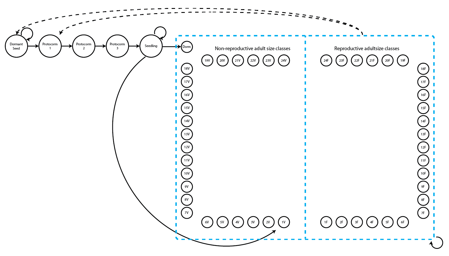
This is a fairly large life history model with two adult life stages for each number of sprouts - a reproductive stage that flowers and a non-reproductive stage that does not flower. Let’s load the raw dataset and set up the stageframe first.
data(cypdata)

stagevector <- c("SD", "P1", "P2", "P3", "SL", "Dorm", "1V", "2V", "3V", "4V",
  "5V", "6V", "7V", "8V", "9V", "10V", "11V", "12V", "13V", "14V", "15V", "16V",
  "17V", "18V", "19V", "20V", "21V", "22V", "23V", "24V", "1F", "2F", "3F",
  "4F", "5F", "6F", "7F", "8F", "9F", "10F", "11F", "12F", "13F", "14F", "15F",
  "16F", "17F", "18F", "19F", "20F", "21F", "22F", "23F", "24F")
indataset <- c(0, 0, 0, 0, 0, rep(1, 49))
sizevector <- c(0, 0, 0, 0, 0, seq(from = 0, t = 24), seq(from = 1, to = 24))
repvector <- c(0, 0, 0, 0, 0, rep(0, 25), rep(1, 24))
obsvector <- c(0, 0, 0, 0, 0, 0, rep(1, 48))
matvector <- c(0, 0, 0, 0, 0, rep(1, 49))
immvector <- c(0, 1, 1, 1, 1, rep(0, 49))
propvector <- c(1, rep(0, 53))
comments <- c("Dormant seed", "Yr1 protocorm", "Yr2 protocorm", "Yr3 protocorm",
  "Seedling", "Veg dorm", "Veg adult 1 stem", "Veg adult 2 stems",
  "Veg adult 3 stems", "Veg adult 4 stems", "Veg adult 5 stems",
  "Veg adult 6 stems", "Veg adult 7 stems", "Veg adult 8 stems",
  "Veg adult 9 stems", "Veg adult 10 stems", "Veg adult 11 stems",
  "Veg adult 12 stems", "Veg adult 13 stems", "Veg adult 14 stems",
  "Veg adult 15 stems", "Veg adult 16 stems", "Veg adult 17 stems",
  "Veg adult 18 stems", "Veg adult 19 stems", "Veg adult 20 stems",
  "Veg adult 21 stems", "Veg adult 22 stems", "Veg adult 23 stems",
  "Veg adult 24 stems", "Flo adult 1 stem", "Flo adult 2 stems",
  "Flo adult 3 stems", "Flo adult 4 stems", "Flo adult 5 stems",
  "Flo adult 6 stems", "Flo adult 7 stems", "Flo adult 8 stems",
  "Flo adult 9 stems", "Flo adult 10 stems", "Flo adult 11 stems",
  "Flo adult 12 stems", "Flo adult 13 stems", "Flo adult 14 stems",
  "Flo adult 15 stems", "Flo adult 16 stems", "Flo adult 17 stems",
  "Flo adult 18 stems", "Flo adult 19 stems", "Flo adult 20 stems",
  "Flo adult 21 stems", "Flo adult 22 stems", "Flo adult 23 stems",
  "Flo adult 24 stems")

cypframe_fb <- sf_create(sizes = sizevector, stagenames = stagevector,
  repstatus = repvector, obsstatus = obsvector, matstatus = matvector,
  propstatus = propvector, immstatus = immvector, indataset = indataset,
  comments = comments)
Now let’s standardize the dataset into a historically formatted vertical (hfv) data frame. We will also need to introduce our annual covariate, total annual precipitation. These data were derived from the National Centers for Environmental Information and the U.S. National Oceanic and Atmospheric Administration. We can either incorporate this variable as a series of individual covariates in our vertical dataset, or use the core dataset without these data and introduce them in the modelsearch() call as an annual covariate. We will insert these climatic data as constants into the data frame holding the dataset so that we can illustrate the former approach.
cypdata_env <- cypdata
cypdata_env$prec.04 <- 92.2
cypdata_env$prec.05 <- 57.6
cypdata_env$prec.06 <- 96.0
cypdata_env$prec.07 <- 109.8
cypdata_env$prec.08 <- 111.9
cypdata_env$prec.09 <- 106.8

cypfb_env <- verticalize3(data = cypdata_env, noyears = 6, firstyear = 2004,
  patchidcol = "patch", individcol = "plantid", blocksize = 4,
  sizeacol = "Inf2.04", sizebcol = "Inf.04", sizeccol = "Veg.04",
  repstracol = "Inf.04", repstrbcol = "Inf2.04", fecacol = "Pod.04",
  indcovacol = c("prec.04", "prec.05", "prec.06", "prec.07", "prec.08",
    "prec.09"), stageassign = cypframe_fb, stagesize = "sizeadded",
  NAas0 = TRUE, age_offset = 4)

summary_hfv(cypfb_env, full = TRUE)
>
> This hfv dataset contains 320 rows, 60 variables, 1 population,
> 3 patches, 74 individuals, and 5 time steps.
>      rowid          popid           patchid    individ           year2
>  Min.   : 1.00   Length:320         A: 93   Min.   : 164.0   Min.   :2004
>  1st Qu.:21.00   Class :character   B:154   1st Qu.: 391.0   1st Qu.:2005
>  Median :37.50   Mode  :character   C: 73   Median : 453.0   Median :2006
>  Mean   :38.45                              Mean   : 651.5   Mean   :2006
>  3rd Qu.:56.00                              3rd Qu.: 476.0   3rd Qu.:2007
>  Max.   :77.00                              Max.   :1560.0   Max.   :2008
>    firstseen       lastseen        obsage       obslifespan
>  Min.   :2004   Min.   :2004   Min.   :5.000   Min.   :0.000
>  1st Qu.:2004   1st Qu.:2009   1st Qu.:6.000   1st Qu.:5.000
>  Median :2004   Median :2009   Median :7.000   Median :5.000
>  Mean   :2004   Mean   :2009   Mean   :6.853   Mean   :4.556
>  3rd Qu.:2004   3rd Qu.:2009   3rd Qu.:8.000   3rd Qu.:5.000
>  Max.   :2008   Max.   :2009   Max.   :9.000   Max.   :5.000
>      sizea1             sizeb1            sizec1       size1added
>  Min.   :0.000000   Min.   : 0.0000   Min.   : 0.0   Min.   : 0.000
>  1st Qu.:0.000000   1st Qu.: 0.0000   1st Qu.: 0.0   1st Qu.: 0.000
>  Median :0.000000   Median : 0.0000   Median : 1.0   Median : 2.000
>  Mean   :0.009375   Mean   : 0.7469   Mean   : 1.9   Mean   : 2.656
>  3rd Qu.:0.000000   3rd Qu.: 1.0000   3rd Qu.: 3.0   3rd Qu.: 4.000
>  Max.   :1.000000   Max.   :18.0000   Max.   :13.0   Max.   :21.000
>     repstra1          repstrb1         repstr1added         feca1
>  Min.   : 0.0000   Min.   :0.000000   Min.   : 0.0000   Min.   :0.0000
>  1st Qu.: 0.0000   1st Qu.:0.000000   1st Qu.: 0.0000   1st Qu.:0.0000
>  Median : 0.0000   Median :0.000000   Median : 0.0000   Median :0.0000
>  Mean   : 0.7469   Mean   :0.009375   Mean   : 0.7562   Mean   :0.2656
>  3rd Qu.: 1.0000   3rd Qu.:0.000000   3rd Qu.: 1.0000   3rd Qu.:0.0000
>  Max.   :18.0000   Max.   :1.000000   Max.   :18.0000   Max.   :7.0000
>    fec1added         indcova1        obsstatus1       repstatus1
>  Min.   :0.0000   Min.   :  0.00   Min.   :0.0000   Min.   :0.0000
>  1st Qu.:0.0000   1st Qu.: 57.60   1st Qu.:0.0000   1st Qu.:0.0000
>  Median :0.0000   Median : 92.20   Median :1.0000   Median :0.0000
>  Mean   :0.2656   Mean   : 70.64   Mean   :0.7469   Mean   :0.2875
>  3rd Qu.:0.0000   3rd Qu.: 96.00   3rd Qu.:1.0000   3rd Qu.:1.0000
>  Max.   :7.0000   Max.   :109.80   Max.   :1.0000   Max.   :1.0000
>    fecstatus1       matstatus1         alive1          stage1
>  Min.   :0.0000   Min.   :0.0000   Min.   :0.0000   Length:320
>  1st Qu.:0.0000   1st Qu.:1.0000   1st Qu.:1.0000   Class :character
>  Median :0.0000   Median :1.0000   Median :1.0000   Mode  :character
>  Mean   :0.1344   Mean   :0.7688   Mean   :0.7688
>  3rd Qu.:0.0000   3rd Qu.:1.0000   3rd Qu.:1.0000
>  Max.   :1.0000   Max.   :1.0000   Max.   :1.0000
>   stage1index        sizea2             sizeb2            sizec2
>  Min.   : 0.00   Min.   :0.000000   Min.   : 0.0000   Min.   : 0.000
>  1st Qu.: 6.00   1st Qu.:0.000000   1st Qu.: 0.0000   1st Qu.: 1.000
>  Median : 8.00   Median :0.000000   Median : 0.0000   Median : 2.000
>  Mean   :14.17   Mean   :0.009375   Mean   : 0.8969   Mean   : 2.416
>  3rd Qu.:31.00   3rd Qu.:0.000000   3rd Qu.: 1.0000   3rd Qu.: 3.000
>  Max.   :51.00   Max.   :1.000000   Max.   :18.0000   Max.   :13.000
>    size2added        repstra2          repstrb2         repstr2added
>  Min.   : 0.000   Min.   : 0.0000   Min.   :0.000000   Min.   : 0.0000
>  1st Qu.: 1.000   1st Qu.: 0.0000   1st Qu.:0.000000   1st Qu.: 0.0000
>  Median : 2.000   Median : 0.0000   Median :0.000000   Median : 0.0000
>  Mean   : 3.322   Mean   : 0.8969   Mean   :0.009375   Mean   : 0.9062
>  3rd Qu.: 4.000   3rd Qu.: 1.0000   3rd Qu.:0.000000   3rd Qu.: 1.0000
>  Max.   :24.000   Max.   :18.0000   Max.   :1.000000   Max.   :18.0000
>      feca2          fec2added         indcova2        obsstatus2
>  Min.   :0.0000   Min.   :0.0000   Min.   : 57.60   Min.   :0.0000
>  1st Qu.:0.0000   1st Qu.:0.0000   1st Qu.: 92.20   1st Qu.:1.0000
>  Median :0.0000   Median :0.0000   Median : 96.00   Median :1.0000
>  Mean   :0.2906   Mean   :0.2906   Mean   : 92.77   Mean   :0.9531
>  3rd Qu.:0.0000   3rd Qu.:0.0000   3rd Qu.:109.80   3rd Qu.:1.0000
>  Max.   :7.0000   Max.   :7.0000   Max.   :111.90   Max.   :1.0000
>    repstatus2       fecstatus2       matstatus2     alive2     stage2
>  Min.   :0.0000   Min.   :0.0000   Min.   :1    Min.   :1   Length:320
>  1st Qu.:0.0000   1st Qu.:0.0000   1st Qu.:1    1st Qu.:1   Class :character
>  Median :0.0000   Median :0.0000   Median :1    Median :1   Mode  :character
>  Mean   :0.3688   Mean   :0.1562   Mean   :1    Mean   :1
>  3rd Qu.:1.0000   3rd Qu.:0.0000   3rd Qu.:1    3rd Qu.:1
>  Max.   :1.0000   Max.   :1.0000   Max.   :1    Max.   :1
>   stage2index        sizea3             sizeb3           sizec3
>  Min.   : 6.00   Min.   :0.000000   Min.   : 0.000   Min.   : 0.000
>  1st Qu.: 7.00   1st Qu.:0.000000   1st Qu.: 0.000   1st Qu.: 1.000
>  Median :10.00   Median :0.000000   Median : 0.000   Median : 1.000
>  Mean   :18.17   Mean   :0.009375   Mean   : 1.069   Mean   : 2.209
>  3rd Qu.:32.00   3rd Qu.:0.000000   3rd Qu.: 1.000   3rd Qu.: 3.000
>  Max.   :54.00   Max.   :1.000000   Max.   :18.000   Max.   :13.000
>    size3added        repstra3         repstrb3         repstr3added
>  Min.   : 0.000   Min.   : 0.000   Min.   :0.000000   Min.   : 0.000
>  1st Qu.: 1.000   1st Qu.: 0.000   1st Qu.:0.000000   1st Qu.: 0.000
>  Median : 2.000   Median : 0.000   Median :0.000000   Median : 0.000
>  Mean   : 3.288   Mean   : 1.069   Mean   :0.009375   Mean   : 1.078
>  3rd Qu.: 4.000   3rd Qu.: 1.000   3rd Qu.:0.000000   3rd Qu.: 1.000
>  Max.   :24.000   Max.   :18.000   Max.   :1.000000   Max.   :18.000
>      feca3          fec3added         indcova3       obsstatus3    repstatus3
>  Min.   :0.0000   Min.   :0.0000   Min.   : 57.6   Min.   :0.0   Min.   :0.0
>  1st Qu.:0.0000   1st Qu.:0.0000   1st Qu.: 96.0   1st Qu.:1.0   1st Qu.:0.0
>  Median :0.0000   Median :0.0000   Median :106.8   Median :1.0   Median :0.0
>  Mean   :0.4562   Mean   :0.4562   Mean   : 96.1   Mean   :0.9   Mean   :0.4
>  3rd Qu.:0.0000   3rd Qu.:0.0000   3rd Qu.:109.8   3rd Qu.:1.0   3rd Qu.:1.0
>  Max.   :8.0000   Max.   :8.0000   Max.   :111.9   Max.   :1.0   Max.   :1.0
>    fecstatus3       matstatus3     alive3          stage3
>  Min.   :0.0000   Min.   :1    Min.   :0.0000   Length:320
>  1st Qu.:0.0000   1st Qu.:1    1st Qu.:1.0000   Class :character
>  Median :0.0000   Median :1    Median :1.0000   Mode  :character
>  Mean   :0.2219   Mean   :1    Mean   :0.9469
>  3rd Qu.:0.0000   3rd Qu.:1    3rd Qu.:1.0000
>  Max.   :1.0000   Max.   :1    Max.   :1.0000
>   stage3index
>  Min.   : 0.00
>  1st Qu.: 7.00
>  Median :10.00
>  Mean   :18.57
>  3rd Qu.:33.00
>  Max.   :54.00
Now we will load the ahistorical supplement table that we will use for the ahistorical projections. We will not work with the historical version with f_projection3() in this chapter due to the increased amount of processing time required for the historical modelsearch() run.
seeds_per_fruit <- 5000 # Mean number of seeds per fruit
sl_mult <- 0.7 # Product of assumed germination prob and survival to 1st year

cypsupp2_fb <- supplemental(stage3 = c("SD", "P1", "P2", "P3", "SL", "SL",
    "Dorm", "1V", "2V", "3V", "SD", "P1"),
  stage2 = c("SD", "SD", "P1", "P2", "P3", "SL", "SL", "SL", "SL", "SL", "rep",
    "rep"),
  eststage3 = c(NA, NA, NA, NA, NA, NA, "Dorm", "1V", "2V", "3V", NA, NA),
  eststage2 = c(NA, NA, NA, NA, NA, NA, "Dorm", "Dorm", "Dorm", "Dorm", NA, NA),
  givenrate = c(0.08, 0.1, 0.1, 0.1, 0.05, 0.05, NA, NA, NA, NA, NA, NA),
  multiplier = c(NA, NA, NA, NA, NA, NA, sl_mult, sl_mult, sl_mult, sl_mult,
    0.5 * seeds_per_fruit, 0.5 * seeds_per_fruit),
  type = c("S", "S", "S", "S", "S", "S", "S", "S", "S", "S", "R", "R"),
  stageframe = cypframe_fb, historical = FALSE)
> Warning: NA values in argument multiplier will be treated as 1 values.

cypsupp2_fb
>    stage3 stage2 stage1 age2 eststage3 eststage2 eststage1 estage2 givenrate
> 1      SD     SD   <NA>   NA      <NA>      <NA>      <NA>      NA      0.08
> 2      P1     SD   <NA>   NA      <NA>      <NA>      <NA>      NA      0.10
> 3      P2     P1   <NA>   NA      <NA>      <NA>      <NA>      NA      0.10
> 4      P3     P2   <NA>   NA      <NA>      <NA>      <NA>      NA      0.10
> 5      SL     P3   <NA>   NA      <NA>      <NA>      <NA>      NA      0.05
> 6      SL     SL   <NA>   NA      <NA>      <NA>      <NA>      NA      0.05
> 7    Dorm     SL   <NA>   NA      Dorm      Dorm      <NA>      NA        NA
> 8      1V     SL   <NA>   NA        1V      Dorm      <NA>      NA        NA
> 9      2V     SL   <NA>   NA        2V      Dorm      <NA>      NA        NA
> 10     3V     SL   <NA>   NA        3V      Dorm      <NA>      NA        NA
> 11     SD    rep   <NA>   NA      <NA>      <NA>      <NA>      NA        NA
> 12     P1    rep   <NA>   NA      <NA>      <NA>      <NA>      NA        NA
>    offset multiplier convtype convtype_t12
> 1      NA        1.0        1            1
> 2      NA        1.0        1            1
> 3      NA        1.0        1            1
> 4      NA        1.0        1            1
> 5      NA        1.0        1            1
> 6      NA        1.0        1            1
> 7      NA        0.7        1            1
> 8      NA        0.7        1            1
> 9      NA        0.7        1            1
> 10     NA        0.7        1            1
> 11     NA     2500.0        3            1
> 12     NA     2500.0        3            1
Next, let’s determine the proper distributions for size and fecundity. As a reminder, size in the Cypripedium dataset is given as the numbers of sprouts, and our proxy for fecundity can be either the number of flowers or the number of fruits produced by an individual. So, size and fecundity in this dataset are all non-negative integers. Count variables generally break the assumptions of the Gaussian distribution because the mean and variance are strongly related, possible values are discrete rather than continuous, and the data distributions are often dramatically skewed. Additionally, because we have absorbed individuals with a size of zero into the dormant stage, there are no zeros left for the size model and so we will need a zero-truncated distribution. Fecundity, in contrast, is a count variable that includes zeros, and so we should test whether we need a zero-inflated model. As for which specific distributions to use, we will use function hfv_qc() to make this determination.
hfv_qc(data = cypfb_env, vitalrates = c("surv", "obs", "size", "repst", "fec"),
  size = c("size3added", "size2added", "size1added"),
  indcova = c("indcova3", "indcova2", "indcova1"))
> Survival:
>
>   Data subset has 61 variables and 320 transitions.
>
>   Variable alive3 has 0 missing values.
>   Variable alive3 is a binomial variable.
>
>   Numbers of categories in data subset in possible random variables:
>   indiv id: 74   (singleton categories: 6)
>   year2: 5   (singleton categories: 0)
>   indcova: 5   (singleton categories: 0)
>
> Observation status:
>
>   Data subset has 61 variables and 303 transitions.
>
>   Variable obsstatus3 has 0 missing values.
>   Variable obsstatus3 is a binomial variable.
>
>   Numbers of categories in data subset in possible random variables:
>   indiv id: 70   (singleton categories: 6)
>   year2: 5   (singleton categories: 0)
>   indcova: 5   (singleton categories: 0)
>
> Primary size:
>
>   Data subset has 61 variables and 288 transitions.
>
>   Variable size3added has 0 missing values.
>   Variable size3added appears to be an integer variable.
>
>   Variable size3added is fully positive, lacking even 0s.
>
>   Overdispersion test:
>     Mean size3added is 3.653
>     The variance in size3added is 13.41
>     The probability of this dispersion level by chance assuming that
>     the true mean size3added = variance in size3added,
>     and an alternative hypothesis of overdispersion, is 3.721e-138
>     Variable size3added is significantly overdispersed.
>
>   Zero-inflation and truncation tests:
>     Mean lambda in size3added is 0.02592
>     The actual number of 0s in size3added is 0
>     The expected number of 0s in size3added under the null hypothesis is 7.465
>     The probability of this deviation in 0s from expectation by chance is 0.9964
>     Variable size3added is not significantly zero-inflated.
>
>     Variable size3added does not include 0s, suggesting that a zero-truncated distribution may be warranted.
>
>   Numbers of categories in data subset in possible random variables:
>   indiv id: 70   (singleton categories: 6)
>   year2: 5   (singleton categories: 0)
>   indcova: 5   (singleton categories: 0)
>
> Reproductive status:
>
>   Data subset has 61 variables and 288 transitions.
>
>   Variable repstatus3 has 0 missing values.
>   Variable repstatus3 is a binomial variable.
>
>   Numbers of categories in data subset in possible random variables:
>   indiv id: 70   (singleton categories: 6)
>   year2: 5   (singleton categories: 0)
>   indcova: 5   (singleton categories: 0)
>
> Fecundity:
>
>   Data subset has 61 variables and 118 transitions.
>
>   Variable feca2 has 0 missing values.
>   Variable feca2 appears to be an integer variable.
>
>   Variable feca2 is fully non-negative.
>
>   Overdispersion test:
>     Mean feca2 is 0.7881
>     The variance in feca2 is 1.536
>     The probability of this dispersion level by chance assuming that
>     the true mean feca2 = variance in feca2,
>     and an alternative hypothesis of overdispersion, is 0.1193
>     Dispersion level in feca2 matches expectation.
>
>   Zero-inflation and truncation tests:
>     Mean lambda in feca2 is 0.4547
>     The actual number of 0s in feca2 is 68
>     The expected number of 0s in feca2 under the null hypothesis is 53.65
>     The probability of this deviation in 0s from expectation by chance is 5.904e-06
>     Variable feca2 is significantly zero-inflated.
>
>   Numbers of categories in data subset in possible random variables:
>   indiv id: 51   (singleton categories: 21)
>   year2: 5   (singleton categories: 0)
>   indcova: 5   (singleton categories: 0)
The results show that size is significantly overdispersed. This means that we cannot use the Poisson distribution, and should instead use the negative binomial distribution. The lack of zeroes in size when zeroes are clearly expected also implies the use of a zero-truncated distribution. Fecundity is not significantly overdispersed, but it is significantly zero-inflated, so we will require a zero-inflated Poisson distribution for that vital rate. All other response variables appear to match the expectations of the binomial distribution, and so are fine.
Now we will run function modelsearch() and find the right parameterizations for our vital rates. We can use either the individual or annual covariate approach to do so. First, let’s try the former, as it provides a more general approach that allows individuals to vary even within years. To achieve this, we need to include indcova = c("indcova3", "indcova2", "indcova1") and test.indcova = TRUE in order to make sure that modelsearch() includes our individual covariate, which reflects total annual precipitation. Including the former argument but not the latter will result in modelsearch() ignoring the individual covariate. If this covariate was categorical and random, then we would also need to stipulate random.indcova = TRUE (our individual covariate is actually quantitative and numerical, so we will use the default setting of FALSE, instead). To prevent this function from taking too long to run, we will drop the patch term, set suite = "main" to prevent the inclusion of interaction terms, and run only an ahistorical set.
cypmodels2_env1 <- modelsearch(cypfb_env, historical = FALSE, approach = "mixed",
  vitalrates = c("surv", "obs", "size", "repst", "fec"), sizedist = "negbin",
  size.trunc = TRUE, fecdist = "poisson", fec.zero = TRUE, suite = "main",
  size = c("size3added", "size2added", "size1added"), test.indcova = TRUE,
  indcova = c("indcova3", "indcova2", "indcova1"), quiet = "partial")
Let’s see the model summaries.
summary(cypmodels2_env1)
> This LefkoMod object includes 5 linear models.
> Best-fit model criterion used: aicc&k
>
>
>
> Survival model:
> Generalized linear mixed model fit by maximum likelihood (Laplace
>   Approximation) [glmerMod]
>  Family: binomial  ( logit )
> Formula: alive3 ~ indcova2 + (1 | year2) + (1 | individ)
>    Data: surv.data
>       AIC       BIC    logLik -2*log(L)  df.resid
>  102.9757  118.0490  -47.4878   94.9757       316
> Random effects:
>  Groups  Name        Std.Dev.
>  individ (Intercept) 1197.97
>  year2   (Intercept)   89.74
> Number of obs: 320, groups:  individ, 74; year2, 5
> Fixed Effects:
> (Intercept)     indcova2
>      271.32        -2.19
> optimizer (Nelder_Mead) convergence code: 0 (OK) ; 0 optimizer warnings; 2 lme4 warnings
>
>
>
> Observation model:
> Generalized linear mixed model fit by maximum likelihood (Laplace
>   Approximation) [glmerMod]
>  Family: binomial  ( logit )
> Formula: obsstatus3 ~ size2added + (1 | year2) + (1 | individ)
>    Data: obs.data
>       AIC       BIC    logLik -2*log(L)  df.resid
>  118.2567  133.1117  -55.1284  110.2567       299
> Random effects:
>  Groups  Name        Std.Dev.
>  individ (Intercept) 1.078e-05
>  year2   (Intercept) 8.776e-01
> Number of obs: 303, groups:  individ, 70; year2, 5
> Fixed Effects:
> (Intercept)   size2added
>      2.4904       0.3134
> optimizer (Nelder_Mead) convergence code: 0 (OK) ; 0 optimizer warnings; 1 lme4 warnings
>
>
>
> Size model:
> Formula:          size3added ~ (1 | year2) + (1 | individ)
> Data: size.data
>       AIC       BIC    logLik -2*log(L)  df.resid
> 1008.2764 1022.9282 -500.1382 1000.2764       284
> Random-effects (co)variances:
>
> Conditional model:
>  Groups  Name        Std.Dev.
>  year2   (Intercept) 0.1109
>  individ (Intercept) 1.0561
>
> Number of obs: 288 / Conditional model: year2, 5; individ, 70
>
> Dispersion parameter for truncated_nbinom2 family (): 1.99e+07
>
> Fixed Effects:
>
> Conditional model:
> (Intercept)
>      0.5761
>
>
>
> Secondary size model:
> [1] 1
>
>
>
> Tertiary size model:
> [1] 1
>
>
>
> Reproductive status model:
> Generalized linear mixed model fit by maximum likelihood (Laplace
>   Approximation) [glmerMod]
>  Family: binomial  ( logit )
> Formula: repstatus3 ~ indcova2 + repstatus2 + size2added + (1 | year2) +
>     (1 | individ)
>    Data: repst.data
>       AIC       BIC    logLik -2*log(L)  df.resid
>  330.0418  352.0196 -159.0209  318.0418       282
> Random effects:
>  Groups  Name        Std.Dev.
>  individ (Intercept) 0.0002695
>  year2   (Intercept) 0.2479120
> Number of obs: 288, groups:  individ, 70; year2, 5
> Fixed Effects:
> (Intercept)     indcova2   repstatus2   size2added
>    -4.23766      0.02954      1.71091      0.17187
>
>
>
> Fecundity model:
> Formula:          feca2 ~ indcova2 + size2added + (1 | year2) + (1 | individ)
> Zero inflation:         ~size2added + (1 | year2) + (1 | individ)
> Data: fec.data
>       AIC       BIC    logLik -2*log(L)  df.resid
>  245.4867  270.4229 -113.7434  227.4867       109
> Random-effects (co)variances:
>
> Conditional model:
>  Groups  Name        Std.Dev.
>  year2   (Intercept) 0.2517
>  individ (Intercept) 0.1927
>
> Zero-inflation model:
>  Groups  Name        Std.Dev.
>  year2   (Intercept) 2.072e-04
>  individ (Intercept) 3.951e-08
>
> Number of obs: 118 / Conditional model: year2, 5; individ, 51 / Zero-inflation model: year2, 5; individ, 51
>
> Fixed Effects:
>
> Conditional model:
> (Intercept)     indcova2   size2added
>     1.68997     -0.02397      0.06174
>
> Zero-inflation model:
> (Intercept)   size2added
>       3.927       -1.618
>
>
> Juvenile survival model:
> [1] 1
>
>
>
> Juvenile observation model:
> [1] 1
>
>
>
> Juvenile size model:
> [1] 1
>
>
>
> Juvenile secondary size model:
> [1] 1
>
>
>
> Juvenile tertiary size model:
> [1] 1
>
>
>
> Juvenile reproduction model:
> [1] 1
>
>
>
> Juvenile maturity model:
> [1] 1
>
>
>
>
>
> Number of models in survival table: 7
>
> Number of models in observation table: 8
>
> Number of models in size table: 8
>
> Number of models in secondary size table: 1
>
> Number of models in tertiary size table: 1
>
> Number of models in reproduction status table: 8
>
> Number of models in fecundity table: 64
>
> Number of models in juvenile survival table: 1
>
> Number of models in juvenile observation table: 1
>
> Number of models in juvenile size table: 1
>
> Number of models in juvenile secondary size table: 1
>
> Number of models in juvenile tertiary size table: 1
>
> Number of models in juvenile reproduction table: 1
>
> Number of models in juvenile maturity table: 1
>
>
>
>
>
> General model parameter names (column 1), and
> specific names used in these models (column 2):
>                       parameter_names mainparams
> 1                              time t      year2
> 2                          individual    individ
> 3                               patch      patch
> 4                   alive in time t+1      surv3
> 5                observed in time t+1       obs3
> 6                   sizea in time t+1      size3
> 7                   sizeb in time t+1     sizeb3
> 8                   sizec in time t+1     sizec3
> 9     reproductive status in time t+1     repst3
> 10              fecundity in time t+1       fec3
> 11                fecundity in time t       fec2
> 12                    sizea in time t      size2
> 13                  sizea in time t-1      size1
> 14                    sizeb in time t     sizeb2
> 15                  sizeb in time t-1     sizeb1
> 16                    sizec in time t     sizec2
> 17                  sizec in time t-1     sizec1
> 18      reproductive status in time t     repst2
> 19    reproductive status in time t-1     repst1
> 20        maturity status in time t+1     matst3
> 21          maturity status in time t     matst2
> 22                      age in time t        age
> 23                  density in time t    density
> 24   individual covariate a in time t   indcova2
> 25 individual covariate a in time t-1   indcova1
> 26   individual covariate b in time t   indcovb2
> 27 individual covariate b in time t-1   indcovb1
> 28   individual covariate c in time t   indcovc2
> 29 individual covariate c in time t-1   indcovc1
> 30              stage group in time t     group2
> 31            stage group in time t-1     group1
> 32       annual covariate a in time t  annucova2
> 33     annual covariate a in time t-1  annucova1
> 34       annual covariate b in time t  annucovb2
> 35     annual covariate b in time t-1  annucovb1
> 36       annual covariate c in time t  annucovc2
> 37     annual covariate c in time t-1  annucovc1
>
>
>
>
>
> Quality control:
>
> Survival model estimated with 74 individuals and 320 individual transitions.
> Survival model accuracy is 1.
> Observation status model estimated with 70 individuals and 303 individual transitions.
> Observation status model accuracy is 0.95.
> Primary size model estimated with 70 individuals and 288 individual transitions.
> Primary size model R-squared is 0.822.
> Secondary size model not estimated.
> Tertiary size model not estimated.
> Reproductive status model estimated with 70 individuals and 288 individual transitions.
> Reproductive status model accuracy is 0.719.
> Fecundity model estimated with 51 individuals and 118 individual transitions.
> Fecundity model R-squared is 0.524.
> Juvenile survival model not estimated.
> Juvenile observation status model not estimated.
> Juvenile primary size model not estimated.
> Juvenile secondary size model not estimated.
> Juvenile tertiary size model not estimated.
> Juvenile reproductive status model not estimated.
> Juvenile maturity status model not estimated.
Total annual precipitation is a factor in the best-fit models of survival, reproductive status, and fecundity, suggesting that it is quite important to the demography of the population. The accuracy scores of our survival, observation status, and size models are really excellent, while the other models have poor to reasonable accuracy or R2.
To illustrate the differences in set-up when using annual covariates, let’s try the same exercise as before but using the annucov series of arguments rather than the indcov series of argument. Let’s try modelsearch() first, using the dataset without any environmental covariates added. Instead, we will enter a vector of precipitation values.
annual_precip <- c(92.2, 57.6, 96.0, 109.8, 111.9)

cypmodels2_anna1 <- modelsearch(cypfb_env, historical = FALSE, approach = "mixed",
  vitalrates = c("surv", "obs", "size", "repst", "fec"), sizedist = "negbin",
  size.trunc = TRUE, fecdist = "poisson", fec.zero = TRUE, suite = "main",
  size = c("size3added", "size2added", "size1added"), test.annucova = TRUE,
  annucova = annual_precip, quiet = "partial")
Let’s see the model summaries.
summary(cypmodels2_anna1)
> This LefkoMod object includes 5 linear models.
> Best-fit model criterion used: aicc&k
>
>
>
> Survival model:
> Generalized linear mixed model fit by maximum likelihood (Laplace
>   Approximation) [glmerMod]
>  Family: binomial  ( logit )
> Formula: alive3 ~ annucova2 + (1 | year2) + (1 | individ)
>    Data: surv.data
>       AIC       BIC    logLik -2*log(L)  df.resid
>  102.9757  118.0490  -47.4878   94.9757       316
> Random effects:
>  Groups  Name        Std.Dev.
>  individ (Intercept) 1197.97
>  year2   (Intercept)   89.74
> Number of obs: 320, groups:  individ, 74; year2, 5
> Fixed Effects:
> (Intercept)    annucova2
>      271.32        -2.19
> optimizer (Nelder_Mead) convergence code: 0 (OK) ; 0 optimizer warnings; 2 lme4 warnings
>
>
>
> Observation model:
> Generalized linear mixed model fit by maximum likelihood (Laplace
>   Approximation) [glmerMod]
>  Family: binomial  ( logit )
> Formula: obsstatus3 ~ size2added + (1 | year2) + (1 | individ)
>    Data: obs.data
>       AIC       BIC    logLik -2*log(L)  df.resid
>  118.2567  133.1117  -55.1284  110.2567       299
> Random effects:
>  Groups  Name        Std.Dev.
>  individ (Intercept) 1.078e-05
>  year2   (Intercept) 8.776e-01
> Number of obs: 303, groups:  individ, 70; year2, 5
> Fixed Effects:
> (Intercept)   size2added
>      2.4904       0.3134
> optimizer (Nelder_Mead) convergence code: 0 (OK) ; 0 optimizer warnings; 1 lme4 warnings
>
>
>
> Size model:
> Formula:          size3added ~ (1 | year2) + (1 | individ)
> Data: size.data
>       AIC       BIC    logLik -2*log(L)  df.resid
> 1008.2764 1022.9282 -500.1382 1000.2764       284
> Random-effects (co)variances:
>
> Conditional model:
>  Groups  Name        Std.Dev.
>  year2   (Intercept) 0.1109
>  individ (Intercept) 1.0561
>
> Number of obs: 288 / Conditional model: year2, 5; individ, 70
>
> Dispersion parameter for truncated_nbinom2 family (): 1.99e+07
>
> Fixed Effects:
>
> Conditional model:
> (Intercept)
>      0.5761
>
>
>
> Secondary size model:
> [1] 1
>
>
>
> Tertiary size model:
> [1] 1
>
>
>
> Reproductive status model:
> Generalized linear mixed model fit by maximum likelihood (Laplace
>   Approximation) [glmerMod]
>  Family: binomial  ( logit )
> Formula: repstatus3 ~ annucova2 + repstatus2 + size2added + (1 | year2) +
>     (1 | individ)
>    Data: repst.data
>       AIC       BIC    logLik -2*log(L)  df.resid
>  330.0418  352.0196 -159.0209  318.0418       282
> Random effects:
>  Groups  Name        Std.Dev.
>  individ (Intercept) 0.0002695
>  year2   (Intercept) 0.2479120
> Number of obs: 288, groups:  individ, 70; year2, 5
> Fixed Effects:
> (Intercept)    annucova2   repstatus2   size2added
>    -4.23766      0.02954      1.71091      0.17187
>
>
>
> Fecundity model:
> Formula:          feca2 ~ annucova2 + size2added + (1 | year2) + (1 | individ)
> Zero inflation:         ~size2added + (1 | year2) + (1 | individ)
> Data: fec.data
>       AIC       BIC    logLik -2*log(L)  df.resid
>  245.4867  270.4229 -113.7434  227.4867       109
> Random-effects (co)variances:
>
> Conditional model:
>  Groups  Name        Std.Dev.
>  year2   (Intercept) 0.2517
>  individ (Intercept) 0.1927
>
> Zero-inflation model:
>  Groups  Name        Std.Dev.
>  year2   (Intercept) 2.072e-04
>  individ (Intercept) 3.951e-08
>
> Number of obs: 118 / Conditional model: year2, 5; individ, 51 / Zero-inflation model: year2, 5; individ, 51
>
> Fixed Effects:
>
> Conditional model:
> (Intercept)    annucova2   size2added
>     1.68997     -0.02397      0.06174
>
> Zero-inflation model:
> (Intercept)   size2added
>       3.927       -1.618
>
>
> Juvenile survival model:
> [1] 1
>
>
>
> Juvenile observation model:
> [1] 1
>
>
>
> Juvenile size model:
> [1] 1
>
>
>
> Juvenile secondary size model:
> [1] 1
>
>
>
> Juvenile tertiary size model:
> [1] 1
>
>
>
> Juvenile reproduction model:
> [1] 1
>
>
>
> Juvenile maturity model:
> [1] 1
>
>
>
>
>
> Number of models in survival table: 7
>
> Number of models in observation table: 8
>
> Number of models in size table: 8
>
> Number of models in secondary size table: 1
>
> Number of models in tertiary size table: 1
>
> Number of models in reproduction status table: 8
>
> Number of models in fecundity table: 64
>
> Number of models in juvenile survival table: 1
>
> Number of models in juvenile observation table: 1
>
> Number of models in juvenile size table: 1
>
> Number of models in juvenile secondary size table: 1
>
> Number of models in juvenile tertiary size table: 1
>
> Number of models in juvenile reproduction table: 1
>
> Number of models in juvenile maturity table: 1
>
>
>
>
>
> General model parameter names (column 1), and
> specific names used in these models (column 2):
>                       parameter_names mainparams
> 1                              time t      year2
> 2                          individual    individ
> 3                               patch      patch
> 4                   alive in time t+1      surv3
> 5                observed in time t+1       obs3
> 6                   sizea in time t+1      size3
> 7                   sizeb in time t+1     sizeb3
> 8                   sizec in time t+1     sizec3
> 9     reproductive status in time t+1     repst3
> 10              fecundity in time t+1       fec3
> 11                fecundity in time t       fec2
> 12                    sizea in time t      size2
> 13                  sizea in time t-1      size1
> 14                    sizeb in time t     sizeb2
> 15                  sizeb in time t-1     sizeb1
> 16                    sizec in time t     sizec2
> 17                  sizec in time t-1     sizec1
> 18      reproductive status in time t     repst2
> 19    reproductive status in time t-1     repst1
> 20        maturity status in time t+1     matst3
> 21          maturity status in time t     matst2
> 22                      age in time t        age
> 23                  density in time t    density
> 24   individual covariate a in time t   indcova2
> 25 individual covariate a in time t-1   indcova1
> 26   individual covariate b in time t   indcovb2
> 27 individual covariate b in time t-1   indcovb1
> 28   individual covariate c in time t   indcovc2
> 29 individual covariate c in time t-1   indcovc1
> 30              stage group in time t     group2
> 31            stage group in time t-1     group1
> 32       annual covariate a in time t  annucova2
> 33     annual covariate a in time t-1  annucova1
> 34       annual covariate b in time t  annucovb2
> 35     annual covariate b in time t-1  annucovb1
> 36       annual covariate c in time t  annucovc2
> 37     annual covariate c in time t-1  annucovc1
>
>
>
>
>
> Quality control:
>
> Survival model estimated with 74 individuals and 320 individual transitions.
> Survival model accuracy is 1.
> Observation status model estimated with 70 individuals and 303 individual transitions.
> Observation status model accuracy is 0.95.
> Primary size model estimated with 70 individuals and 288 individual transitions.
> Primary size model R-squared is 0.822.
> Secondary size model not estimated.
> Tertiary size model not estimated.
> Reproductive status model estimated with 70 individuals and 288 individual transitions.
> Reproductive status model accuracy is 0.719.
> Fecundity model estimated with 51 individuals and 118 individual transitions.
> Fecundity model R-squared is 0.524.
> Juvenile survival model not estimated.
> Juvenile observation status model not estimated.
> Juvenile primary size model not estimated.
> Juvenile secondary size model not estimated.
> Juvenile tertiary size model not estimated.
> Juvenile reproductive status model not estimated.
> Juvenile maturity status model not estimated.
We have the exact same models as in the individual covariate case, only using the variable name annucova instead of indcova.
Now that we have developed our vital rate models, let’s also build vectors showing our expectation for shifts in the precipitation over the next 20 years from the year that data collection stopped. This 20 year period will be our main time window of interest for projection. Our climate values will be real predictions from Shefferson et al. (2017), which were extracted from a climate forecast model maintained by Japan’s National Meteorological Research Institute. We will use the values predicted for 2010 to 2030. Just out of interest, we will also create a vector of predicted values for 2070 to 2090.
pred_vals_2010to30 <- c(110.8152136, 98.87159542, 127.0623005, 110.0501797,
  82.03005742, 103.6893125, 104.2549713, 97.86989854, 111.25054, 116.4481035,
  125.9652504, 98.89823738, 105.7075192, 135.7032496, 149.6705465, 149.0110188,
  115.3965537, 119.7017105, 99.5415225, 111.7898123, 90.51828146)

pred_vals_2070to90 <- c(101.7828506, 80.70954521, 106.760383, 142.3355673,
  113.6519693, 122.3257958, 100.8745268, 138.814026, 111.1349475, 92.00440938,
  120.2391638, 115.6253448, 102.6373673, 125.3819469, 98.25464504, 102.4367633,
  118.6401779, 125.6021119, 101.9117747, 127.2149739, 109.244138)
Let’s see what these values look like graphically (figure 8.3).
plot(x = c(1:21), y = pred_vals_2010to30, type = "l", lty = 1, lwd = 3,
  ylab = "Annual precip (cm)", xlab = "Projected year", ylim = c(80, 170),
  bty = "n")
lines(x = c(1:21), y = pred_vals_2070to90, lty = 2, lwd = 3)
legend("topright", c("2010-2030", "2070-2090"), lty = c(1, 2), lwd = 3,
  bty = "n")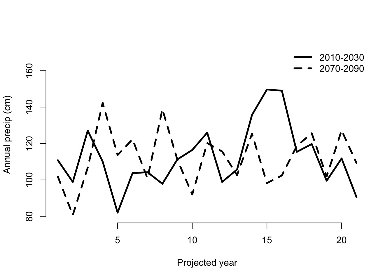
Figure 8.3: Predicted annual precipitation for Cypripedium candidum
We see some interesting, rather cyclical patterns. Now let’s move on to conducting our projection analyses.
8.2 Simple projections of already developed matrices for a specific time length
One of the most common forms of projection analysis involves projecting an arithmetic mean matrix deterministically. Perhaps we wish to project the mean forward by ten time steps simply to see the short-term predicted trend, or perhaps we wish to project many thousands of time steps in order to see the asymptotic properties of the matrix. Let’s start off by building arithmetic mean matrices for the ahistorical and historical population-level MPMs.
cypmean2 <- lmean(cypmatrix2r)
cypmean3 <- lmean(cypmatrix3r)

summary(cypmean2)
>
> This ahistorical lefkoMat object contains 1 matrix.
>
> Each matrix is square with 11 rows and columns, and a total of 121 elements.
> A total of 33 survival transitions were estimated, with 33 per matrix.
> A total of 10 fecundity transitions were estimated, with 10 per matrix.
> This lefkoMat object covers 1 population, 1 patch, and 0 time steps.
>
> The dataset contains a total of 74 unique individuals and 320 unique transitions.
>
> Survival probability sum check (each matrix represented by column in order):
>          [,1]
> Min.    0.050
> 1st Qu. 0.140
> Median  0.800
> Mean    0.593
> 3rd Qu. 0.921
> Max.    1.000
>
>
> All matrices have no stage discontinuities.

summary(cypmean3)
>
> This historical lefkoMat object contains 1 matrix.
>
> Each matrix is square with 121 rows and columns, and a total of 14641 elements.
> A total of 99 survival transitions were estimated, with 99 per matrix.
> A total of 28 fecundity transitions were estimated, with 28 per matrix.
> This lefkoMat object covers 1 population, 1 patch, and 0 time steps.
>
> The dataset contains a total of 74 unique individuals and 320 unique transitions.
>
> Survival probability sum check (each matrix represented by column in order):
>          [,1]
> Min.    0.000
> 1st Qu. 0.000
> Median  0.000
> Mean    0.179
> 3rd Qu. 0.200
> Max.    1.000
>
>
> Stage-pairs without connections leading to them found in matrices: 1
Now let’s project these two mean matrices forward. Since these are only single matrices, we do not need to indicate any specific year or patch to project. We will instruct R to project the ahistorical mean ten time steps forward. Then, we will take a look at the resulting object.
cypproj2 <- projection3(cypmean2, times = 10)
> Warning: This lefkoMat object appears to be a set of mean matrices. Will
> project only the mean.

cypproj2
> $projection
> $projection[[1]]
> $projection[[1]][[1]]
>       [,1]         [,2]         [,3]         [,4]         [,5]         [,6]
>  [1,]    1 1.025278e+04 8976.9428602 7579.2162919 6559.5257069 5791.2902872
>  [2,]    1 1.025280e+04 9181.9984786 7758.7551491 6711.1100327 5922.4808013
>  [3,]    1 1.000000e-01 1025.2800919  918.1998479  775.8755149  671.1110033
>  [4,]    1 1.000000e-01    0.0100000  102.5280092   91.8199848   77.5875515
>  [5,]    1 1.000000e-01    0.0100000    0.0010000    5.1264505    4.8473218
>  [6,]    1 2.326441e-01    0.2158192    0.2037291    0.1945073    0.4237303
>  [7,]    1 1.496794e+00    1.3301888    1.2290474    1.1663551    2.9546675
>  [8,]    1 1.804320e+00    1.8827350    1.8582091    1.7999057    2.7390456
>  [9,]    1 8.390066e-01    0.8995651    0.9136912    0.8912658    0.8505446
> [10,]    1 1.075116e+00    0.9570211    0.8349439    0.7303300    0.6449596
> [11,]    1 5.952381e-01    0.4000111    0.2911504    0.2250937    0.1821021
>               [,7]         [,8]         [,9]        [,10]        [,11]
>  [1,] 5777.0586419 6330.3074391 7144.4860609 8023.4195510 8864.9356819
>  [2,] 5892.8844477 6445.8486120 7271.0922097 8166.3092722 9025.4040729
>  [3,]  592.2480801  589.2884448  644.5848612  727.1092210  816.6309272
>  [4,]   67.1111003   59.2248080   58.9288445   64.4584861   72.7109221
>  [5,]    4.1217437    3.5616422    3.1393225    3.1034083    3.3780947
>  [6,]    0.5946490    0.6972683    0.7576925    0.7932213    0.8270709
>  [7,]    4.0352491    4.6021723    4.9080956    5.0742834    5.2639516
>  [8,]    3.7343588    4.5180195    5.0926985    5.5058964    5.8572084
>  [9,]    0.9816220    1.2047260    1.4431232    1.6600921    1.8434275
> [10,]    0.6345045    0.6788768    0.7530879    0.8390462    0.9253580
> [11,]    0.1524758    0.1366669    0.1329884    0.1382168    0.1490176
>
>
>
> $stage_dist
> $stage_dist[[1]]
> [1] 0
>
>
> $rep_value
> $rep_value[[1]]
> [1] 0
>
>
> $pop_size
> $pop_size[[1]]
>      [,1]     [,2]     [,3]     [,4]     [,5]     [,6]     [,7]     [,8]
> [1,]   11 20511.92 19189.93 16364.03 14148.47 12475.11 12343.56 13440.07
>          [,9]    [,10]    [,11]
> [1,] 15135.32 16998.41 18797.93
>
>
> $labels
>   pop patch
> 1   1     1
>
> $ahstages
>    stage_id stage original_size original_size_b original_size_c min_age max_age
> 1         1    SD           0.0              NA              NA       0      NA
> 2         2    P1           0.0              NA              NA       0      NA
> 3         3    P2           0.0              NA              NA       0      NA
> 4         4    P3           0.0              NA              NA       0      NA
> 5         5    SL           0.0              NA              NA       0      NA
> 6         6  Dorm           0.0              NA              NA       0      NA
> 7         7   XSm           1.0              NA              NA       0      NA
> 8         8    Sm           3.0              NA              NA       0      NA
> 9         9    Md           6.0              NA              NA       0      NA
> 10       10    Lg          11.0              NA              NA       0      NA
> 11       11   XLg          19.5              NA              NA       0      NA
>    repstatus obsstatus propstatus immstatus matstatus entrystage indataset
> 1          0         0          1         0         0          1         0
> 2          0         0          0         1         0          1         0
> 3          0         0          0         1         0          0         0
> 4          0         0          0         1         0          0         0
> 5          0         0          0         1         0          0         0
> 6          0         0          0         0         1          0         1
> 7          1         1          0         0         1          0         1
> 8          1         1          0         0         1          0         1
> 9          1         1          0         0         1          0         1
> 10         1         1          0         0         1          0         1
> 11         1         1          0         0         1          0         1
>    binhalfwidth_raw sizebin_min sizebin_max sizebin_center sizebin_width
> 1               0.0         0.0         0.0            0.0             0
> 2               0.0         0.0         0.0            0.0             0
> 3               0.0         0.0         0.0            0.0             0
> 4               0.0         0.0         0.0            0.0             0
> 5               0.0         0.0         0.0            0.0             0
> 6               0.5        -0.5         0.5            0.0             1
> 7               0.5         0.5         1.5            1.0             1
> 8               1.5         1.5         4.5            3.0             3
> 9               1.5         4.5         7.5            6.0             3
> 10              3.5         7.5        14.5           11.0             7
> 11              5.0        14.5        24.5           19.5            10
>    binhalfwidthb_raw sizebinb_min sizebinb_max sizebinb_center sizebinb_width
> 1                 NA           NA           NA              NA             NA
> 2                 NA           NA           NA              NA             NA
> 3                 NA           NA           NA              NA             NA
> 4                 NA           NA           NA              NA             NA
> 5                 NA           NA           NA              NA             NA
> 6                 NA           NA           NA              NA             NA
> 7                 NA           NA           NA              NA             NA
> 8                 NA           NA           NA              NA             NA
> 9                 NA           NA           NA              NA             NA
> 10                NA           NA           NA              NA             NA
> 11                NA           NA           NA              NA             NA
>    binhalfwidthc_raw sizebinc_min sizebinc_max sizebinc_center sizebinc_width
> 1                 NA           NA           NA              NA             NA
> 2                 NA           NA           NA              NA             NA
> 3                 NA           NA           NA              NA             NA
> 4                 NA           NA           NA              NA             NA
> 5                 NA           NA           NA              NA             NA
> 6                 NA           NA           NA              NA             NA
> 7                 NA           NA           NA              NA             NA
> 8                 NA           NA           NA              NA             NA
> 9                 NA           NA           NA              NA             NA
> 10                NA           NA           NA              NA             NA
> 11                NA           NA           NA              NA             NA
>    group                       comments alive almostborn
> 1      0                   Dormant seed     1          0
> 2      0               1st yr protocorm     1          0
> 3      0               2nd yr protocorm     1          0
> 4      0               3rd yr protocorm     1          0
> 5      0                       Seedling     1          0
> 6      0                  Dormant adult     1          0
> 7      0    Extra small adult (1 shoot)     1          0
> 8      0       Small adult (2-4 shoots)     1          0
> 9      0      Medium adult (5-7 shoots)     1          0
> 10     0      Large adult (8-14 shoots)     1          0
> 11     0 Extra large adult (>14 shoots)     1          0
>
> $hstages
>   X1
> 1 NA
>
> $agestages
>   X1
> 1 NA
>
> $control
> [1]  1 10
>
> attr(,"class")
> [1] "lefkoProj"
Here we can see the structure of the resulting object, which is of class lefkoProj. Its elements include:
- projection - A list with two levels. The top-level elements correspond to the patches or population-patch combinations in the input
lefkoMatobject, with as many elements as there are population-patch combinations (equivalent to the numbers of rows in thelabelsobject). Each of these top-level elements is also a list with number of elements equal to the number of replicates (optionnreps, which defaults to 1). Each element of this lower-level list is a matrix with rows corresponding to the MPM stages (if ahistorical; paired stages if historical; ages if Leslie; and age-stages if age-by-stage), and columns corresponding to the projected times (total number of columns equal to the number of time steps plus 1, with the starting population vector at time 0). The elements of the matrix show the projected number of individuals in the stages, ages, age-stages, or historical stage-pairs in that time. - stage_dist - A list showing the stage distribution projected per time, with the same order and structure as projection. Only estimated if
growthonly = FALSE(the default). - rep_value - A list showing the reproductive value of each stage projected per time, with the same order and structure as projection. Only estimated if
growthonly = FALSE(the default). - pop_size - A list with number of elements equal to the number of projected patches or population-patches. Each element of this list is a matrix showing the total population size at each time (column) per replicate (row).
- labels - A data frame giving the population, patch, and year of each matrix in the
lefkoMatobject used as input, in order. - ahstages - The stageframe used in analysis, though modified and edited according to MPM creation conventions.
- hstages - A data frame matrix showing the pairing of ahistorical stages used to create historical stage pairs (only if historical).
- agestages - A data frame showing the order of age-stage pairs (only if age-by-stage).
- control - An integer vector indicating the number of replicates and the number of time steps.
- density - The data frame input under the density option. Only provided if input by the user.
Let’s also conduct a historical projection, and then compare summaries.
cypproj3 <- projection3(cypmean3, times = 10)
> Warning: This lefkoMat object appears to be a set of mean matrices. Will
> project only the mean.

summary(cypproj2)
>
> The input lefkoProj object covers 1 population-patches.
> It is a single projection including 10 projected steps per replicate, and 1 replicates, respectively.
> The number of replicates with population size above the threshold size of 1 is as in
> the following matrix, with pop-patches given by column and milepost times given by row:
> $milepost_sums
>      1 1
> 0      1
> 0.25   1
> 0.5    1
> 0.75   1
> 1      1
>
> $extinction_times
> [1] NA

summary(cypproj3)
>
> The input lefkoProj object covers 1 population-patches.
> It is a single projection including 10 projected steps per replicate, and 1 replicates, respectively.
> The number of replicates with population size above the threshold size of 1 is as in
> the following matrix, with pop-patches given by column and milepost times given by row:
> $milepost_sums
>      1 1
> 0      1
> 0.25   1
> 0.5    1
> 0.75   1
> 1      1
>
> $extinction_times
> [1] NA
The summary() calls give us a reasonable amount of information, showing the number of population-patches, projected time steps and number of replicates. We also see how many replicates still have population sizes above 1.0 at 0%, 25%, 50%, 75%, and 100% of the way through the projection. A number of options exist for summary() calls with projection3() and f_projection3(), and we encourage the user to explore upon reading the help pages for function summary.lefkoProj.
Let’s also plot the projections for comparison (figure 8.4).
par(mfrow=c(1,2))

plot(cypproj2)
title("a)", adj = 0)

plot(cypproj3, ylab = "")
title("b)", adj = 0)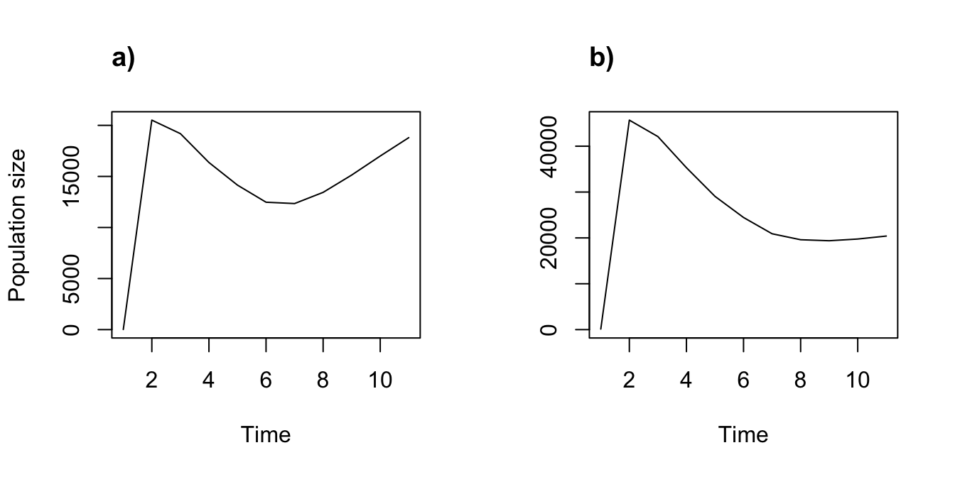
Figure 8.4: Ahistorical (a) vs. historical (b) deterministic projection
These are fascinating results suggesting that accounting for history causes an initial greater spike in population, followed by a more dramatic reduction in the projected population dynamics.
A close look at the population sizes projected at each time shows that decimal values are allowed. Naturally, partial individuals cannot exist in a population. Although the default in lefko3 is to project fractional individuals, we may change the settings to allow only integer values. Doing so results in the projected number of individuals rounding down to the nearest non-negative integer in each time step. We can set this with the integeronly option. Let’s do so and inspect our new projection (figure 8.5).
cypproj3i <- projection3(cypmean3, times = 10, integeronly = TRUE)
> Warning: This lefkoMat object appears to be a set of mean matrices. Will
> project only the mean.

plot(cypproj3i)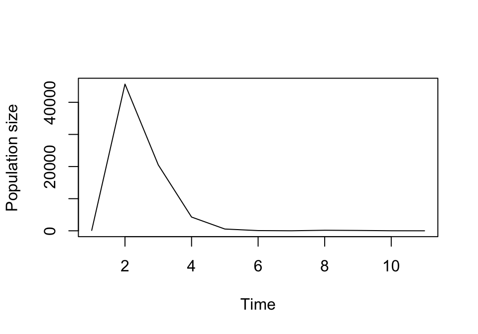
Figure 8.5: Historical projection allowing integer population size only
We will not set integeronly = TRUE in the rest of this chapter, mostly because we are interested predominantly in the overall patterns of population dynamics, and forcing the projection of whole individuals makes extinction more and more likely with smaller population sizes. However, users working with small populations, interested in absolute population numbers, wishing to assess the impacts of individual fate, or exploring the impacts of demographic stochasticity should use this setting.
8.2.1 Setting the start vector
Let’s look at another setting of both functions projection3() and f_projection3(): the start vector. By default, functions projection3() and f_projection3() assume an initial starting vector of one individual in each stage, age (if Leslie), stage pair (if historical), or age-stage (if age-by-stage). We can see this by taking a look at the first column of the core ahistorical projection.
We see above that we started with one individual of each stage. But what if we wished to use a different start vector, for example because we wish to predict future population dynamics on the basis of the stage structure observed currently? In that circumstance, we have two options. The first is to use the start_vec option to load a vector of starting numbers of each stage, stage pair, or age-stage. Here is an example in which we start with 1000 seeds and 100 first-year protocorms, and no individuals of any other stage.
cypproj2_1000 <- projection3(cypmean2, times = 10,
  start_vec = c(1000, 100, 0, 0, 0, 0, 0, 0, 0, 0, 0))
> Warning: This lefkoMat object appears to be a set of mean matrices. Will
> project only the mean.

plot(cypproj2_1000)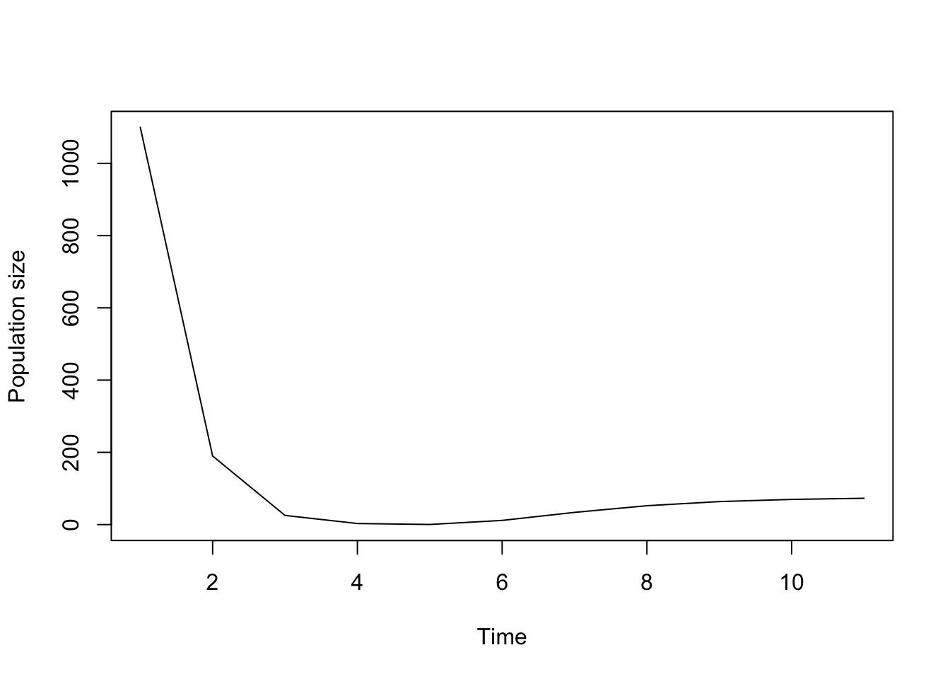
Figure 8.6: Projecting using start_vec to provide an initial start vector
The start_vec approach is very useful, but it requires a vector as long as the number of rows in the projection matrix. This can make it very difficult to create the right start vector for a historical matrix, an age-by-stage matrix, or an IPM. For the latter situations, we can use the start_input() function together with the start_frame option. We use start_input() to create a lefkoSV object, which is a data frame that contains everything we need to know for the start vector. Let’s see this approach in action using a different start vector. Let’s start the population this time with 1000 3rd year protocorms and 100 dormant adults.
c2m_sv <- start_input(cypmean2, stage2 = c("P3", "Dorm"), value = c(1000, 100))
c2m_sv
>   stage2 stage_id_2 stage1 stage_id_1 age2 row_num value
> 1     P3          4     NA         NA   NA       4  1000
> 2   Dorm          6     NA         NA   NA       6   100
In the code above, we told R that we wished to start with 1000 3rdyear protocorms and 100 dormant adults. By not stating any further information, we implied zero individuals for all other stages. The result is this start frame, which is a data frame showing the stages with non-zero starting individuals.
Now that we have our start frame, let’s use it in a projection.
cypproj2_s1000 <- projection3(cypmean2, times = 10, start_frame = c2m_sv)
> Warning: This lefkoMat object appears to be a set of mean matrices. Will
> project only the mean.

plot(cypproj2_s1000)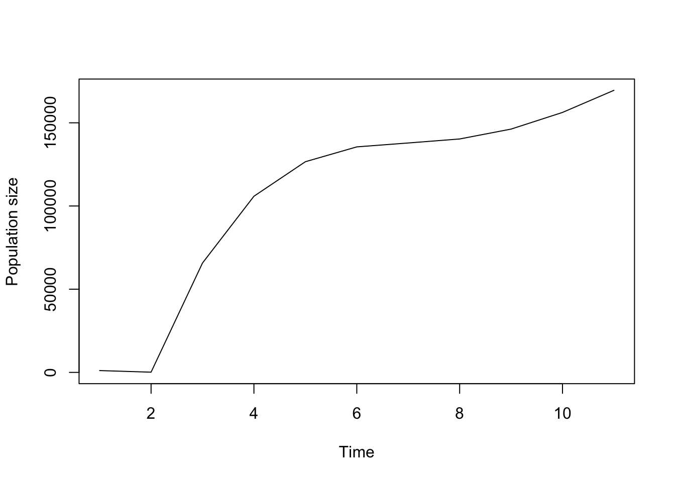
Figure 8.7: Projecting using start_frame to provide an initial start vector
We can compare these projections via a multi-panel plot (figure 8.8).
par(mfrow = c(1, 3))

plot(cypproj2)
title("a)", adj = 0)

plot(cypproj2_1000, ylab = "")
title("b)", adj = 0)

plot(cypproj2_s1000, ylab = "")
title("c)", adj = 0)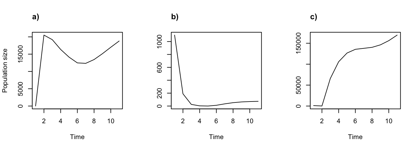
Figure 8.8: Using different starting population vectors. Projections started with (a) 1 of each stage, (b) 1000 dormant seeds and 100 seedlings set via start_vec, and (c) 1000 3rd year protocorms and 100 dormant adults set via start_input
The impact of a different start vector can be quite profound. The leftmost plot shows a population with a single individual of each stage, and so the population is able to grow right away. In contrast, the center and rightmost plots show populations that initially contain no reproductive individuals. In the center plot, it takes a few years for the dormant seeds and 1st year protocorms to mature and the population to start growing. In the rightmost plot, the population starts growing once some of the dormant individuals become reproductive, which takes one or two years.
8.3 Simple projections involving the creation of function-based matrices in each time step
Let’s now switch to function-based projections, which will allow us to create new matrices at each time step using our vital rate models. The first style of function-based projection that we will try is a standard deterministic projection using our individual covariate values. We have two choices - we may either choose a single year to run (our vital rates all include random year terms) with our projected precipitation values, or we may try a specific sequence of years. There are different merits to both approaches. For instructional purposes, let’s start by choosing a single year in the middle of the monitoring - 2007. We also need to format the individual covariate into a three-column data frame with as many rows as we wish to project, and set zero as the default value for unused covariates. Here, we develop our first projection using the 2010 to 2030 predictions. Note that f_projection3() does not calculate mean matrices, unlike function projection3().
ind_frame_1 <- cbind.data.frame(inda = pred_vals_2010to30, indb = 0, indc = 0)

trial2f_1 <- f_projection3(data = cypfb_env, format = 3, stageframe = cypframe_fb,
  supplement = cypsupp2_fb, modelsuite = cypmodels2_env1, times = 21,
  year = 2007, ind_terms = ind_frame_1)
> Warning: Option patch not set, so will set to first patch/population.
The resulting object is of class lefkoProj, just as in the case of function projection3() above. The object includes the same elements as in that case, with the addition of one further element:
- density_vr - The data frame input under the
density_vroption. This data frame shows density dependence per vital rate model, if such information was provided.
We can view a summary of this object as follows. Note that the output is structured in the same way as summary() statement output from lefkoProj objects developed with function projection3().
summary(trial2f_1)
>
> The input lefkoProj object covers 1 population-patches.
> It is a single projection including 21 projected steps per replicate, and 1 replicates, respectively.
> The number of replicates with population size above the threshold size of 1 is as in
> the following matrix, with pop-patches given by column and milepost times given by row:
> $milepost_sums
>      1 1
> 0      1
> 0.25   1
> 0.5    1
> 0.75   1
> 1      1
>
> $extinction_times
> [1] NA
Let’s now also build a projection covering climatic values projected for 2070 to 2090.
ind_frame_2 <- cbind.data.frame(inda = pred_vals_2070to90, indb = 0, indc = 0)

trial2f_2 <- f_projection3(data = cypfb_env, format = 3, stageframe = cypframe_fb,
  supplement = cypsupp2_fb, modelsuite = cypmodels2_env1, times = 21,
  year = 2007, ind_terms = ind_frame_2)
> Warning: Option patch not set, so will set to first patch/population.

summary(trial2f_2)
>
> The input lefkoProj object covers 1 population-patches.
> It is a single projection including 21 projected steps per replicate, and 1 replicates, respectively.
> The number of replicates with population size above the threshold size of 1 is as in
> the following matrix, with pop-patches given by column and milepost times given by row:
> $milepost_sums
>      1 1
> 0      1
> 0.25   1
> 0.5    0
> 0.75   0
> 1      0
>
> $extinction_times
> [1] NA
Now let’s plot our projections side-by-side (figure 8.9).
par(mfrow=c(1,2))

plot(trial2f_1, xlab = "Time from 2010")
title("a)", adj = 0)

plot(trial2f_2, xlab = "Time from 2070", ylab = "")
title("b)", adj = 0)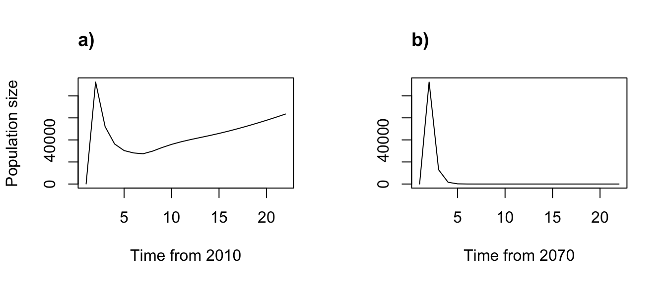
Figure 8.9: Simple function-based projections for (a) 2010-2030 and (b) 2070-2090
Clearly our different climate projections have different impacts on population dynamics.
As an alternative to the previous case, let’s see what happens when we use the annual covariate approach to projection. Here, we perform the same projection, but using our annual covariate lefkoMod object with a slightly restructured data frame of precipitation values. In this case, we need to bind three covariates together into a new data frame, because there are 3 variables that may be used as annual covariates in lefko3. This data frame is then used as input for the ann_terms argument in f_projection3().
annu_frame_2 <- cbind.data.frame(annucova = pred_vals_2070to90, annucovb = 0,
  annucovc = 0)

trial2f_2_1 <- f_projection3(data = cypfb_env, format = 3, stageframe = cypframe_fb,
  supplement = cypsupp2_fb, modelsuite = cypmodels2_anna1, times = 21,
  year = 2007, ann_terms = annu_frame_2)
> Warning: Option patch not set, so will set to first patch/population.

summary(trial2f_2_1)
>
> The input lefkoProj object covers 1 population-patches.
> It is a single projection including 21 projected steps per replicate, and 1 replicates, respectively.
> The number of replicates with population size above the threshold size of 1 is as in
> the following matrix, with pop-patches given by column and milepost times given by row:
> $milepost_sums
>      1 1
> 0      1
> 0.25   1
> 0.5    0
> 0.75   0
> 1      0
>
> $extinction_times
> [1] NA

par(mfrow=c(1,2))

plot(trial2f_2, xlab = "Time from 2070")
title("a)", adj = 0)

plot(trial2f_2_1, xlab = "Time from 2070", ylab = "")
title("b)", adj = 0)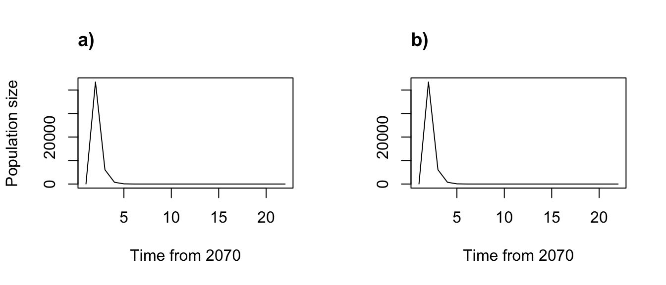
Figure 8.10: Simple function-based projections for 2070-2090 using a) individual and b) annual covariate approaches
Everything looks the same, as it should!
8.3.1 Setting the start vector for function-based projection
As before, we can reset the starting numbers of individuals in different stages. Function f_projection3() assumes one individual per stage at the start by default, similarly to projection3(). As in projection3(), we can set the starting vector with the start_vec and start_frame options. Here we show an example of the latter, which is the more powerful approach. We will start the population with 1000 dormant seeds and 100 1st year protocorms, using the 2010 to 2030 climate projection (figure 8.11). Note that prior to using this option, we need to create a new MPM in the same format as our projection, as the start_input() function will need to look at the structure of the matrices and row / column indices to determine the proper vector.
trial_mpm <- flefko2(data = cypfb_env, stageframe = cypframe_fb,
  supplement = cypsupp2_fb, modelsuite = cypmodels2_env1, year = 2007)

c2m_sv <- start_input(trial_mpm, stage2 = c("SD", "P1"), value = c(1000, 100))

trial2f_3 <- f_projection3(data = cypfb_env, format = 3, stageframe = cypframe_fb,
  supplement = cypsupp2_fb, modelsuite = cypmodels2_env1, times = 21,
  year = 2007, ind_terms = ind_frame_1, start_frame = c2m_sv)
> Warning: Option patch not set, so will set to first patch/population.

par(mfrow = c(1, 2))

plot(trial2f_1)
title("a)", adj = 0)

plot(trial2f_3, ylab = "")
title("b)", adj = 0)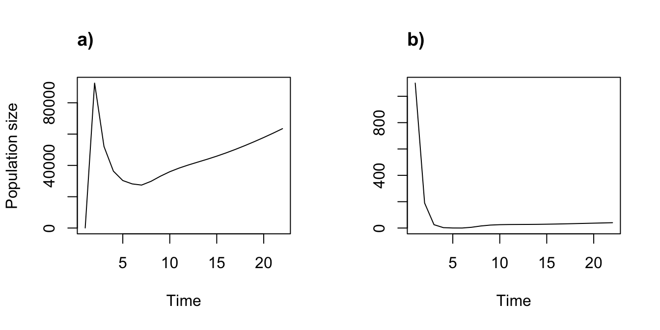
Figure 8.11: Simple function-based projections assuming different start frames. (a) Start with one individual of each stage. (b) Start with 1000 dormant seeds and 100 1st year protocorms
In the new projection, we start the population with dormant seeds and 1st year protocorms only, which means that there is no reproduction in the population for the first few years. This causes an immediate drop in population size until some seeds and protocorms start reproducing. Once reproductive individuals enter the population, population size begins increasing, though much more slowly than in the original projection.
8.4 Ordered / cyclical projections
Situations may arise in which we wish to project an MPM with a specific order of matrices in mind. Typically these situations arise when a specific order of annual matrices is meant to correspond to the assumptions of predicted conditions. For example, we might have several years worth of matrices, with some under high rain conditions and others under drought. We may believe due to climate forecasts that the next ten years should be relatively rainy while the ten years after that should be drier, and may wish to project our matrices forward in an order that matches these expectations. Alternatively, we may have a situation in which a hurricane has affected our population, and we wish to project the population forward avoiding matrices in the immediate aftermath of the hurricane, since those matrices likely reflect dramatic changes as the population adjusts to the mass mortality and other issues that might have destabilized population dynamics during the hurricane itself.
8.4.1 Projecting existing matrices
Let’s start with a scenario in which we have created all of the matrices that we will use, and wish to project them in a specific order. Let’s start by forcing the projection to cycle through the matrices for 2007 and 2008 for ten years, and then to cycle between 2004 and 2005 for another ten years (2004 and 2005 were relatively dry years, while 2007 and 2008 were relatively wet years). Our projection will be 20 years in total.
year_order <- c(2007, 2008, 2007, 2008, 2007, 2008, 2007, 2008, 2007, 2008,
  2004, 2005, 2004, 2005, 2004, 2005, 2004, 2005, 2004, 2005)
cypproj2_ord1 <- projection3(cypmatrix2r, year = year_order, times = 20,
  start_frame = c2m_sv)

summary(cypproj2_ord1)
>
> The input lefkoProj object covers 1 population-patches.
> It is a single projection including 20 projected steps per replicate, and 1 replicates, respectively.
> The number of replicates with population size above the threshold size of 1 is as in
> the following matrix, with pop-patches given by column and milepost times given by row:
> $milepost_sums
>      1 1
> 0      1
> 0.25   1
> 0.5    1
> 0.75   1
> 1      1
>
> $extinction_times
> [1] NA
If we have an MPM with a set of annual matrices, we might wish to project the population forward cyclically through those matrices. If the number of matrices in the lefkoMat object is shorter than the number of time steps set, then the default behavior of lefko3’s projection functions is to cycle through the MPMs. For example, if we leave the times option out from the above projection, then lefko3 will assume the default of 10,000 time steps, and cycle through our 20 defined years over and over, as below.
cypproj2_ord2 <- projection3(cypmatrix2r, year = year_order,
  start_frame = c2m_sv)

summary(cypproj2_ord2)
>
> The input lefkoProj object covers 1 population-patches.
> It is a single projection including 10000 projected steps per replicate, and 1 replicates, respectively.
> The number of replicates with population size above the threshold size of 1 is as in
> the following matrix, with pop-patches given by column and milepost times given by row:
> $milepost_sums
>      1 1
> 0      1
> 0.25   1
> 0.5    1
> 0.75   1
> 1      1
>
> $extinction_times
> [1] NA
Let’s see plots of these projections (figure 8.12).
par(mfrow=c(1,2))

plot(cypproj2_ord1)
title("a)", adj = 0)

plot(cypproj2_ord2, ylab = "")
title("b)", adj = 0)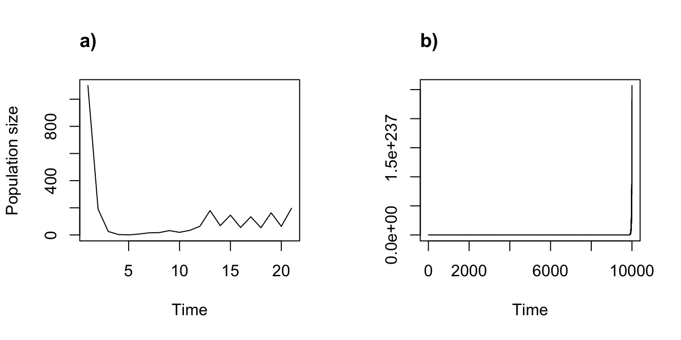
Figure 8.12: Ordered projections can be cyclical. (a) A 20 year ordered projection. (b) A 10,000 year projection cycling through 20 ordered years
Of course, the scales of the x and y axes differ dramatically between these two plots, because both the time scale and the numbers of individuals attained within the projection time period differ dramatically. The population is generally increasing in both cases, and so reaches much greater numbers in 10,000 time steps than in 20.
If the year option is not used and stochastic = FALSE, then the default behavior of this function is to cycle through all matrices in a lefkoMat object in the order that they occur in the labels element. Here, we will cycle through all of the matrices in the ahistorical and historical population-level MPMs for 100 time steps each.
cypproj2_c100 <- projection3(cypmatrix2r, times = 100)
cypproj3_c100 <- projection3(cypmatrix3r, times = 100)

summary(cypproj2_c100)
>
> The input lefkoProj object covers 1 population-patches.
> It is a single projection including 100 projected steps per replicate, and 1 replicates, respectively.
> The number of replicates with population size above the threshold size of 1 is as in
> the following matrix, with pop-patches given by column and milepost times given by row:
> $milepost_sums
>      1 1
> 0      1
> 0.25   1
> 0.5    1
> 0.75   1
> 1      1
>
> $extinction_times
> [1] NA

summary(cypproj3_c100)
>
> The input lefkoProj object covers 1 population-patches.
> It is a single projection including 100 projected steps per replicate, and 1 replicates, respectively.
> The number of replicates with population size above the threshold size of 1 is as in
> the following matrix, with pop-patches given by column and milepost times given by row:
> $milepost_sums
>      1 1
> 0      1
> 0.25   1
> 0.5    1
> 0.75   1
> 1      1
>
> $extinction_times
> [1] NA
Now let’s plot the projections for comparison (figure 8.13).
par(mfrow=c(1,2))

plot(cypproj2_c100)
title("a)", adj = 0)

plot(cypproj3_c100, ylab = "")
title("b)", adj = 0)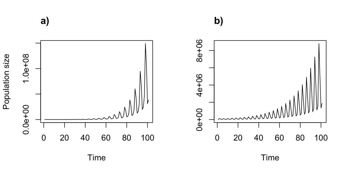
Figure 8.13: Cyclical ahistorical (a) and historical (b) projections
Here we see through comparison of the scales of the y axes that individual history appears to reduce the growth rate relative to ahistorical projection, although clearly there are years in which the population growth rate appears quite high in both cases. The cyclical nature of the projection is obvious in both plots, as it results in noticeable “saw tooth” oscillations over time.
We might also wish to see what happens across different patches. Let’s try a projection with patch structure, here using cypmatrix3rp. This MPM contains four matrices each for three patches.
cypproj3p_c100 <- projection3(cypmatrix3rp, times = 100)

summary(cypproj3p_c100)
>
> The input lefkoProj object covers 4 population-patches.
> It is a single projection including 100 projected steps per replicate, and 1 replicates, respectively.
> The number of replicates with population size above the threshold size of 1 is as in
> the following matrix, with pop-patches given by column and milepost times given by row:
> $milepost_sums
>      1 A 1 B 1 C 1 0
> 0      1   1   1   1
> 0.25   1   1   1   1
> 0.5    1   1   1   1
> 0.75   1   1   1   1
> 1      0   1   1   1
>
> $extinction_times
> [1] NA
Function projection3() has projected the matrix sets from each patch and the patch-weighted population in an ordered cycle for 100 time steps each, with each patch assumed to be independent of every other patch. The summary shows us that patch A goes extinct some time between times 76 and 101. The population-level projection is summarized in the the rightmost column of the milepost_sums, and shows no extinction. Let’s plot these results.
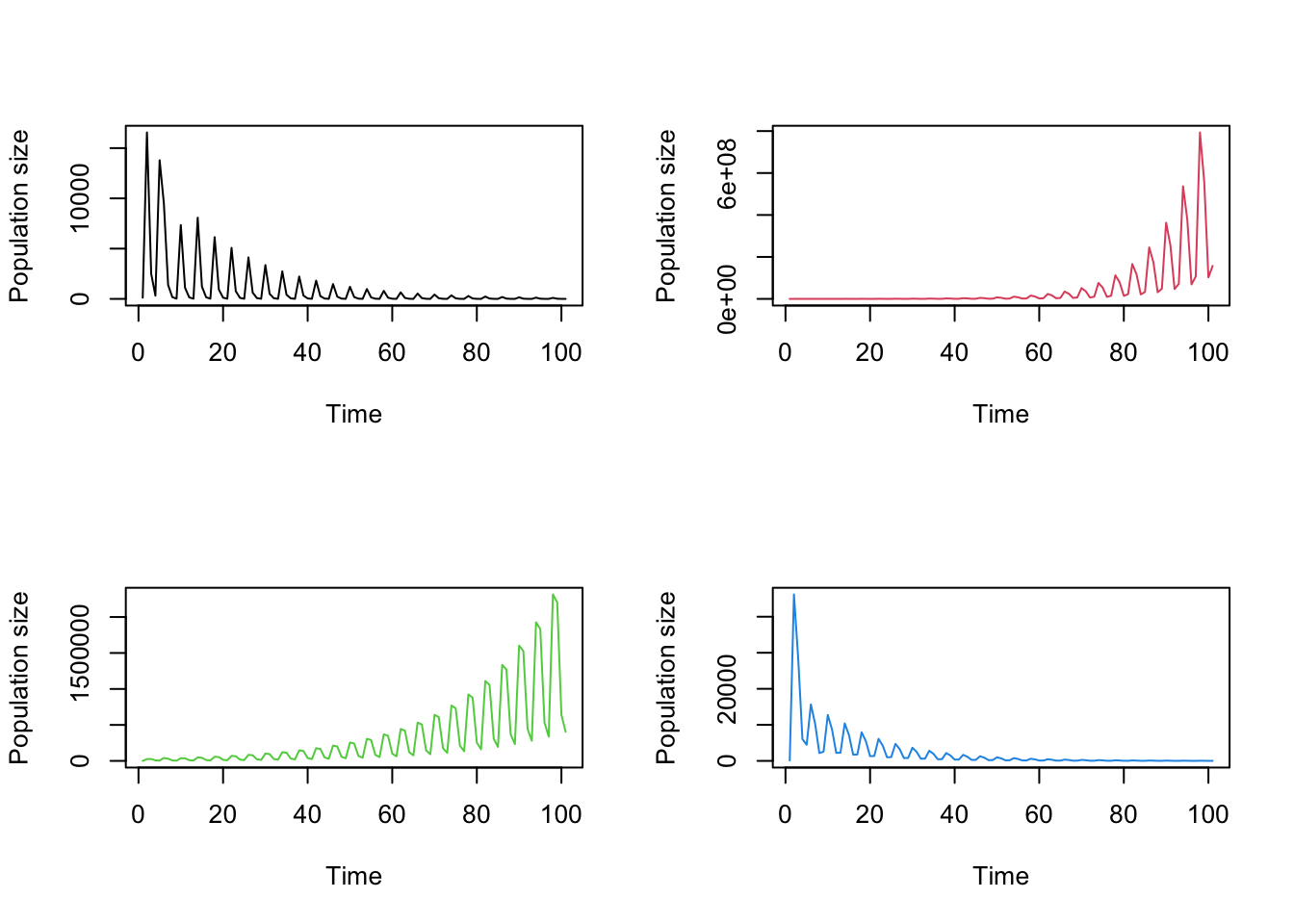
Figure 8.14: Patch-level projections for patch A (top left), patch B (top right), patch C (bottom left), and the patch-weighted population (bottom right)
The plots above are produced in the order of the labels element in the lefkoProj object, which we see below. The plots are propagated by row, meaning that patch A is in the top-left, patch B is in the top-right, patch C is in the bottom-left, and the patch-weighted population mean is in the bottom-right, as shown in the labels element below. These results differ from the population-level projection because the population-level results from a patch-stratified MPM involve averaging the patches equally, whereas a population-level projection weights individual transitions as equal regardless of source patch.
8.4.2 Projecting function-based matrices
The vital rate models developed with modelsearch() generally include year2 terms denoting time t. These are terms within a categorical variable, and so each year has its own value. If we do not specify a specific year to project, then f_projection3() will cycle through the years in the dataset in order for the number of time steps set, using the appropriate year2 term in each vital rate model used to estimate each matrix at each time step. Alternatively, if the year option is set to a vector of years, then these particular years will cycle in order for the number of time steps set. Note, however, that this function only sets the values for the categorical year2 term in the vital rate models - any related terms, such as individual covariates, are unaffected by this and need to be set separately.
Let’s take an example using three years in particular: 2006, 2007, and 2008. By choosing these years and loading this choice as a vector in the year option, we will have lefko3 cycle through them in order. Because our vital rate models also include precipitation, we need to incorporate values for precipitation, and our choices will make a big difference. As in the year case, f_projection3() will cycle though whatever values we provide until the projection is finished. These cycles are independent of the year option cycles, and so care needs to be taken to load only values corresponding to the correct year sequence. Here, we will run three projections using our year vector of three years. Each one will assume a different precipitation input: the first will be a vector of six precipitation values, the second will be just the first of those values, and the third will be the mean of those six values.
ind_real <- data.frame(inda = c(92.2, 57.6, 96.0, 109.8, 111.9, 106.8),
  indb = 0, indc = 0)
short_real <- as.data.frame(ind_real[1,])
mean_real <- data.frame(inda = mean(ind_real$inda), indb = 0, indc = 0)

trial2f_4a <- f_projection3(data = cypfb_env, format = 3, stageframe = cypframe_fb,
  supplement = cypsupp2_fb, modelsuite = cypmodels2_env1, times = 101,
  year = c(2006, 2007, 2008), ind_terms = ind_real)
> Warning: Option patch not set, so will set to first patch/population.
> Warning: Too few values of individual covariates have been supplied. Some will
> be cycled.

trial2f_4b <- f_projection3(data = cypfb_env, format = 3, stageframe = cypframe_fb,
  supplement = cypsupp2_fb, modelsuite = cypmodels2_env1, times = 101,
  year = c(2006, 2007, 2008), ind_terms = short_real)
> Warning: Option patch not set, so will set to first patch/population.
> Warning: Too few values of individual covariates have been supplied. Some will
> be cycled.

trial2f_4c <- f_projection3(data = cypfb_env, format = 3, stageframe = cypframe_fb,
  supplement = cypsupp2_fb, modelsuite = cypmodels2_env1, times = 101,
  year = c(2006, 2007, 2008), ind_terms = mean_real)
> Warning: Option patch not set, so will set to first patch/population.
> Warning: Too few values of individual covariates have been supplied. Some will
> be cycled.

summary(trial2f_4a)
>
> The input lefkoProj object covers 1 population-patches.
> It is a single projection including 101 projected steps per replicate, and 1 replicates, respectively.
> The number of replicates with population size above the threshold size of 1 is as in
> the following matrix, with pop-patches given by column and milepost times given by row:
> $milepost_sums
>      1 1
> 0      1
> 0.25   1
> 0.5    1
> 0.75   1
> 1      1
>
> $extinction_times
> [1] NA

summary(trial2f_4b)
>
> The input lefkoProj object covers 1 population-patches.
> It is a single projection including 101 projected steps per replicate, and 1 replicates, respectively.
> The number of replicates with population size above the threshold size of 1 is as in
> the following matrix, with pop-patches given by column and milepost times given by row:
> $milepost_sums
>      1 1
> 0      1
> 0.25   1
> 0.5    1
> 0.75   1
> 1      1
>
> $extinction_times
> [1] NA

summary(trial2f_4c)
>
> The input lefkoProj object covers 1 population-patches.
> It is a single projection including 101 projected steps per replicate, and 1 replicates, respectively.
> The number of replicates with population size above the threshold size of 1 is as in
> the following matrix, with pop-patches given by column and milepost times given by row:
> $milepost_sums
>      1 1
> 0      1
> 0.25   1
> 0.5    1
> 0.75   1
> 1      1
>
> $extinction_times
> [1] NA
Here is another example using the full set of years instead of a subset, though assuming the same three precipitation vectors as the last runs.
trial2f_5a <- f_projection3(data = cypfb_env, format = 3, stageframe = cypframe_fb,
  supplement = cypsupp2_fb, modelsuite = cypmodels2_env1, times = 101,
  ind_terms = ind_real)
> Warning: Option year not set, so will cycle through existing years.
> Warning: Option patch not set, so will set to first patch/population.
> Warning: Too few values of individual covariates have been supplied. Some will
> be cycled.

trial2f_5b <- f_projection3(data = cypfb_env, format = 3, stageframe = cypframe_fb,
  supplement = cypsupp2_fb, modelsuite = cypmodels2_env1, times = 101,
  ind_terms = short_real)
> Warning: Option year not set, so will cycle through existing years.
> Warning: Option patch not set, so will set to first patch/population.
> Warning: Too few values of individual covariates have been supplied. Some will
> be cycled.

trial2f_5c <- f_projection3(data = cypfb_env, format = 3, stageframe = cypframe_fb,
  supplement = cypsupp2_fb, modelsuite = cypmodels2_env1, times = 101,
  ind_terms = mean_real)
> Warning: Option year not set, so will cycle through existing years.
> Warning: Option patch not set, so will set to first patch/population.
> Warning: Too few values of individual covariates have been supplied. Some will
> be cycled.

summary(trial2f_5a)
>
> The input lefkoProj object covers 1 population-patches.
> It is a single projection including 101 projected steps per replicate, and 1 replicates, respectively.
> The number of replicates with population size above the threshold size of 1 is as in
> the following matrix, with pop-patches given by column and milepost times given by row:
> $milepost_sums
>      1 1
> 0      1
> 0.25   1
> 0.5    1
> 0.75   1
> 1      1
>
> $extinction_times
> [1] NA

summary(trial2f_5b)
>
> The input lefkoProj object covers 1 population-patches.
> It is a single projection including 101 projected steps per replicate, and 1 replicates, respectively.
> The number of replicates with population size above the threshold size of 1 is as in
> the following matrix, with pop-patches given by column and milepost times given by row:
> $milepost_sums
>      1 1
> 0      1
> 0.25   1
> 0.5    1
> 0.75   1
> 1      1
>
> $extinction_times
> [1] NA

summary(trial2f_5c)
>
> The input lefkoProj object covers 1 population-patches.
> It is a single projection including 101 projected steps per replicate, and 1 replicates, respectively.
> The number of replicates with population size above the threshold size of 1 is as in
> the following matrix, with pop-patches given by column and milepost times given by row:
> $milepost_sums
>      1 1
> 0      1
> 0.25   1
> 0.5    1
> 0.75   1
> 1      1
>
> $extinction_times
> [1] NA
Let’s plot the results of all six runs together (figure 8.15).
par(mfrow=c(3,2))

plot(trial2f_4a)
title("a)", adj = 0)

plot(trial2f_4b, ylab = "")
title("b)", adj = 0)

plot(trial2f_4c)
title("c)", adj = 0)

plot(trial2f_5a, ylab = "")
title("d)", adj = 0)

plot(trial2f_5b)
title("e)", adj = 0)

plot(trial2f_5c, ylab = "")
title("f)", adj = 0)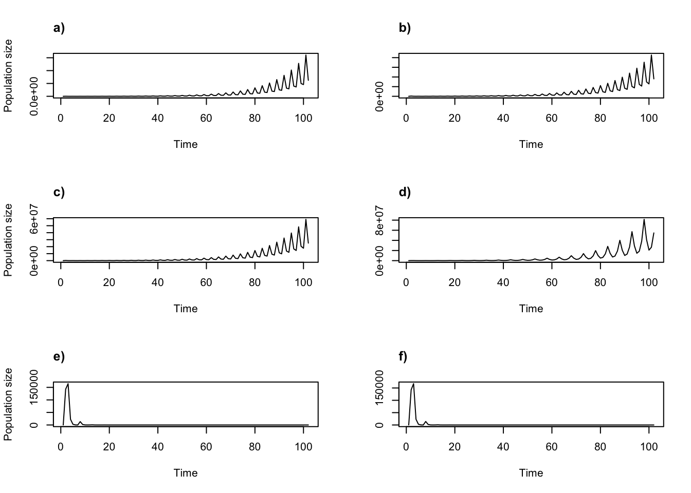
Figure 8.15: Cyclical function-based projections using 2007-2009 only (a, b, c), or all years (d, e, f,), assuming all six real precip values (a, d), precip for 2004 only (b, e), or mean precip over 2004-2009 (d, f).
The choice of which years and individual covariate values led to some interesting differences in the shape of the oscillations.
The approach above can be used to program any particular order of years. The year option should simply be paired with a vector of whatever length showing the order of year terms desired. Here, we use a sequence of years initially switching between years 2007 and 2008, then settling into 2008 for nine years, and ending on year 2005. Let’s assume constant mean precipitation.
year_order <- c(2007, 2008, 2007, 2008, 2007, 2008, 2007, 2008, 2007, 2008,
  2008, 2008, 2008, 2008, 2008, 2008, 2008, 2008, 2008, 2005)

trial2f_6 <- f_projection3(data = cypfb_env, format = 3, stageframe = cypframe_fb,
  supplement = cypsupp2_fb, modelsuite = cypmodels2_env1, year = year_order,
  times = 20, ind_terms = mean_real)
> Warning: Option patch not set, so will set to first patch/population.
> Warning: Too few values of individual covariates have been supplied. Some will
> be cycled.

summary(trial2f_6)
>
> The input lefkoProj object covers 1 population-patches.
> It is a single projection including 20 projected steps per replicate, and 1 replicates, respectively.
> The number of replicates with population size above the threshold size of 1 is as in
> the following matrix, with pop-patches given by column and milepost times given by row:
> $milepost_sums
>      1 1
> 0      1
> 0.25   1
> 0.5    1
> 0.75   1
> 1      1
>
> $extinction_times
> [1] NA
As before, if we set a larger number for times than we will cycle through the sequence.
trial2f_7 <- f_projection3(data = cypfb_env, format = 3, stageframe = cypframe_fb,
  supplement = cypsupp2_fb, modelsuite = cypmodels2_env1, year = year_order,
  times = 100, ind_terms = mean_real)
> Warning: Option patch not set, so will set to first patch/population.
> Warning: Too few values of individual covariates have been supplied. Some will
> be cycled.

summary(trial2f_7)
>
> The input lefkoProj object covers 1 population-patches.
> It is a single projection including 100 projected steps per replicate, and 1 replicates, respectively.
> The number of replicates with population size above the threshold size of 1 is as in
> the following matrix, with pop-patches given by column and milepost times given by row:
> $milepost_sums
>      1 1
> 0      1
> 0.25   1
> 0.5    1
> 0.75   1
> 1      1
>
> $extinction_times
> [1] NA
No extinction happened in either case. Let’s take a look at plots of these projections for further details (figure 8.16).
par(mfrow=c(1, 2))

plot(trial2f_6)
title("a)", adj= 0)

plot(trial2f_7, ylab = "")
title("b)", adj= 0)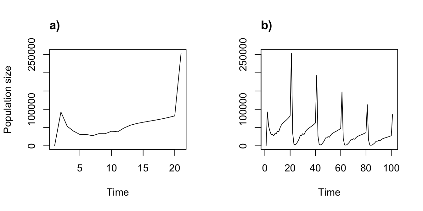
Figure 8.16: Ordered progression of year terms used in projection. (a) Specific sequence of 20 years projected for 20 years. (b) Specific sequence of 20 years projected cyclically for 100 years.
The population appears to grow, and we see that the cycled sequence causes a fairly dramatic and interestingly shaped growth curve.
8.5 Appending projections together
Once constructed, a need might arise to combine some projections into the same output. This generally arises when the same population matrices or function-based MPMs are projected under different conditions, or when sub-populations are run separately and then need to be put back together. Users interested in appending one projection to another can use function append_lP().
Below, we create a new lefkoMat object holding an MPM with only patch A from our original dataset. We then project it forward for 100 time steps, setting the integeronly option so that only integers are possible. Finally, we append this projection to our patch-level projection with all three patches and the mean projected 100 time steps forward.
cypmatrix3r_A <- rlefko3(data = cypraw_v1, stageframe = cypframe_raw,
  year = "all", patch = "A", stages = c("stage3", "stage2", "stage1"),
  size = c("size3added", "size2added", "size1added"), supplement = cypsupp3_raw,
  yearcol = "year2", patchcol = "patchid", indivcol = "individ",
  sparse_output = TRUE)

cypproj3_A_c1000 <- projection3(cypmatrix3r_A, integeronly = TRUE, times = 1000)

cyp_appended <- append_lP(cypproj3p_c100, cypproj3_A_c1000)

summary(cyp_appended)
>
> The input lefkoProj object covers 4 population-patches.
> It is an appended projection, including an average and maximum of 280 and 1000 steps per
> replicate, and an average and maximum of 1.25 and 2 replicates.
> The number of replicates with population size above the threshold size of 1 is as in
> the following matrix, with pop-patches given by column and milepost times given by row:
> $milepost_sums
>      1 A 1 B 1 C 1 0
> 0      2   1   1   1
> 0.25   0   1   1   1
> 0.5    0   1   1   1
> 0.75   0   1   1   1
> 1      0   1   1   1
>
> $extinction_times
> [1] NA
So there are some clear differences in these projections. Let’s plot the combined lefkoProj object.
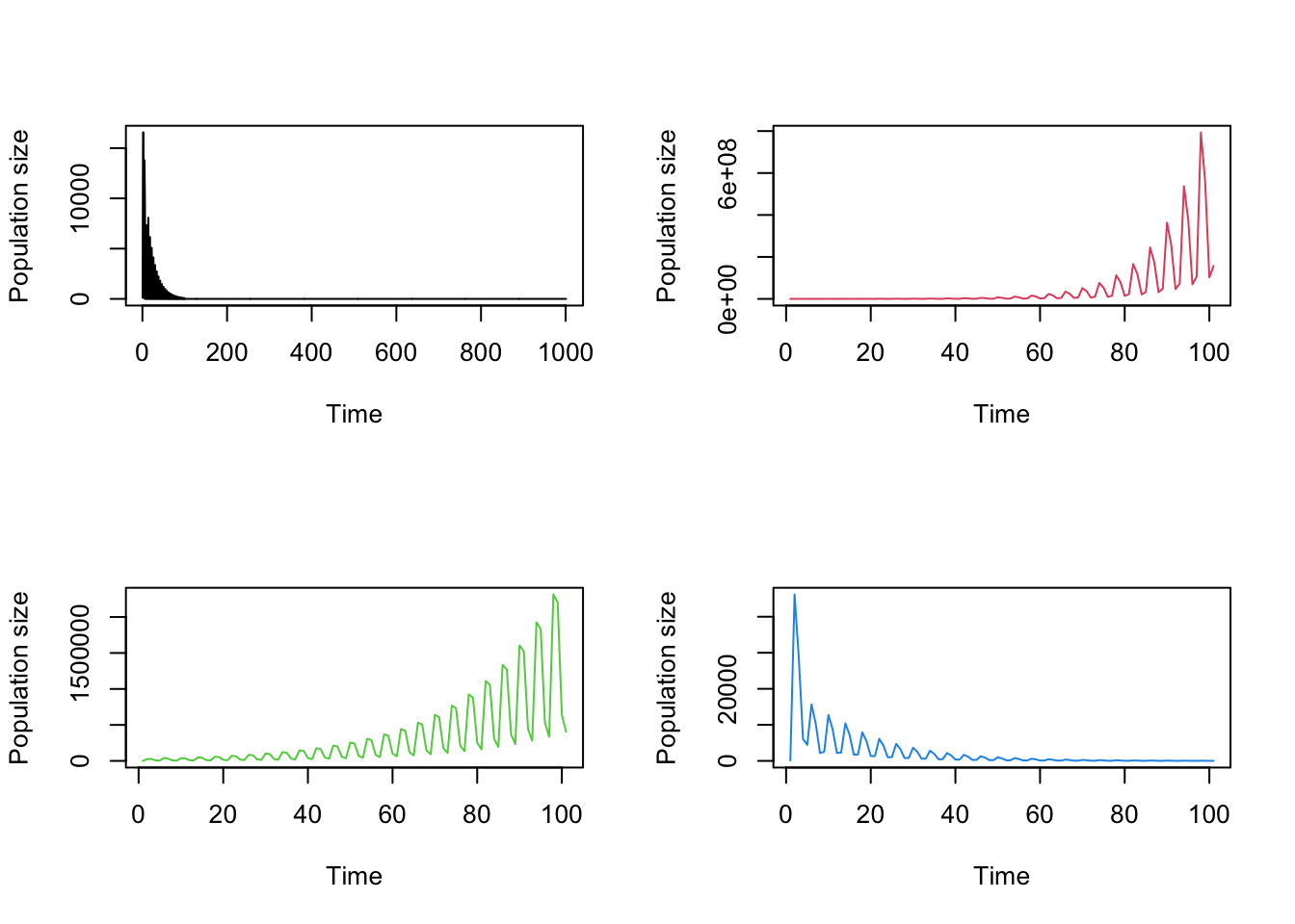
Figure 8.17: Appended projections. a) Patch A shows an appended projection resulting from object cypproj3_A_c1000. b-d) Projections for patches B and C, and the patch-weighted population.
We can see the difference in projection length by comparing the x-axis, with the first projection for 1000 time steps and all others for 100.
8.6 Projections involving bootstrapped data
Projecting bootstrapped MPMs works the same way as creating bootstrapped MPMs. In both empirical and function-based cases, we begin by bootstrapping the hfv dataset. Let’s start with the empirical projection case.
set.seed(42)
cypraw_v1_boot <- bootstrap3(cypraw_v1, reps = 10)

summary_hfv(cypraw_v1_boot)
>
> This hfvlist object contains 10 hfvdata demographic data frames.
> Each data frame contains an average of 316.7 rows, 57 variables, 1 population,
> 3 patches, 46.3 individuals, and 5 time steps.
>
> Across all data frames, there are 1 unique population, 3 unique patches, 74 unique individuals, and 5 unique time steps.
Next, we will create our bootstrapped matrices.
cypmatrix2r_boot <- rlefko2(data = cypraw_v1_boot, stageframe = cypframe_raw,
  year = "all", stages = c("stage3", "stage2"),
  size = c("size3added", "size2added"), supplement = cypsupp2_raw,
  yearcol = "year2", indivcol = "individ")

summary(cypmatrix2r_boot)
>
> This lefkoMatList object contains 10 ahistorical lefkoMat objects.
> The average lefkoMat object contains 5 matrices.
>
> This lefkoMatList object covers an average of 1 population, 1 patch, and 5 time steps.
> Each matrix is square with 11 rows and columns, and a total of 121 elements.
> An average of 108.1 survival transitions were estimated in each lefkoMat object,
> with an average of 21.62 per matrix.
> An average of 33.2 fecundity transitions were estimated in each lefkoMat object,
> with an average of 6.64 per matrix.
>
> The datasets contain an average total of 48 unique individuals and 318 unique transitions.
Finally, we run the empirical projection, using the same function and format as before, but using the bootstrapped MPMs.
cypproj2_boot <- projection3(cypmatrix2r_boot, times = 25)

class(cypproj2_boot)
> [1] "lefkoProjList"
summary(cypproj2_boot)
>       Length Class     Mode
>  [1,] 9      lefkoProj list
>  [2,] 9      lefkoProj list
>  [3,] 9      lefkoProj list
>  [4,] 9      lefkoProj list
>  [5,] 9      lefkoProj list
>  [6,] 9      lefkoProj list
>  [7,] 9      lefkoProj list
>  [8,] 9      lefkoProj list
>  [9,] 9      lefkoProj list
> [10,] 9      lefkoProj list
The summary() function shows us a standard R list summary, and we can see that the result is a lefkoProjList object with 10 elements, each of which is a lefkoProj object. We can take a look at what these bootstrapped projections look like by applying all of the functions that we have used so far, but to the elements of this list. For example, let’s plot the population sizes of the first 4 bootstrapped projection.
par(mfrow = c(2, 2))

plot(cypproj2_boot[[1]])
plot(cypproj2_boot[[2]])
plot(cypproj2_boot[[3]])
plot(cypproj2_boot[[4]])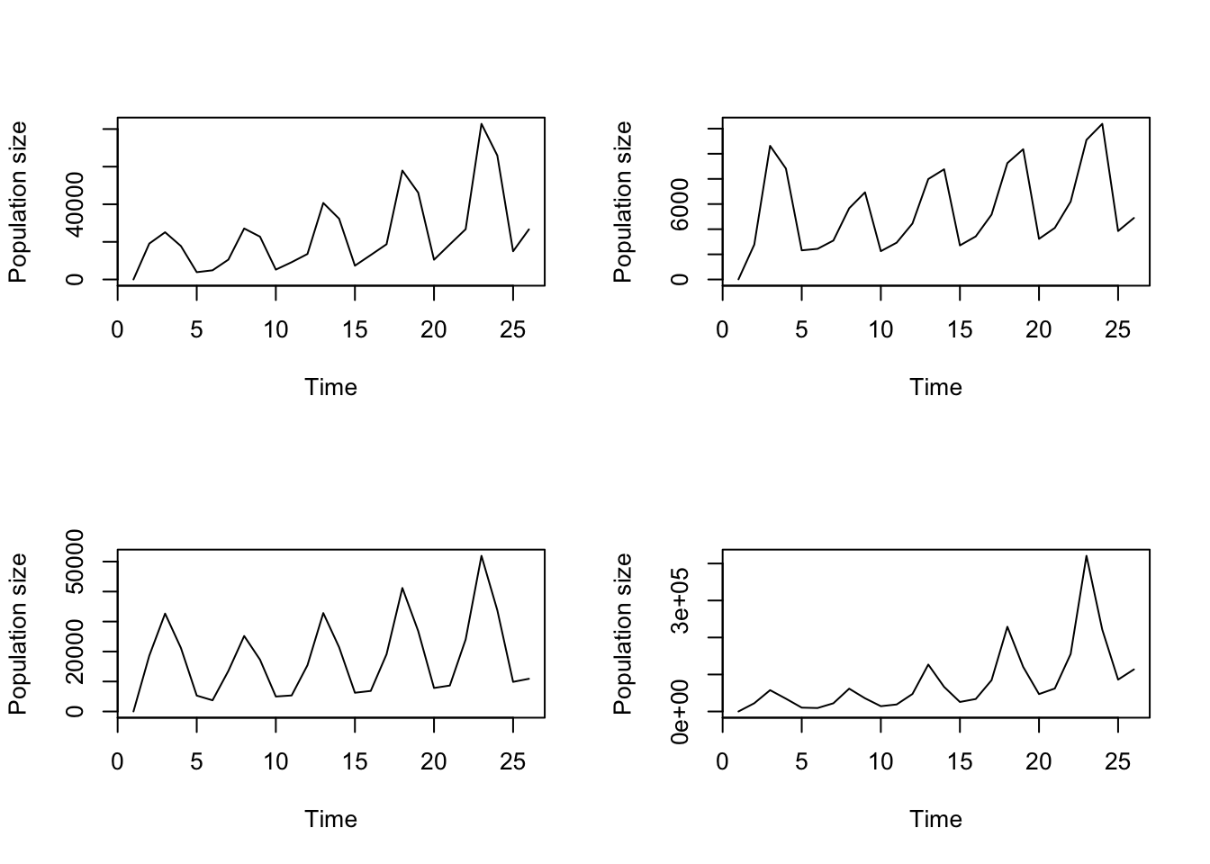
Figure 8.18: Raw, ahistorical bootstrapped projections of Cypripedium candidum
Let’s now take a look at function-based bootstrapped projections. As before, we will start off by bootstrapping the dataset to get as many bootstrapped replicates as we would like.
set.seed(42)
cypfb_env_boot <- bootstrap3(cypfb_env, reps = 5)

summary_hfv(cypfb_env_boot)
>
> This hfvlist object contains 5 hfvdata demographic data frames.
> Each data frame contains an average of 313.4 rows, 60 variables, 1 population,
> 3 patches, 47 individuals, and 5 time steps.
>
> Across all data frames, there are 1 unique population, 3 unique patches, 73 unique individuals, and 5 unique time steps.
Next, as with function-based MPM creation, we need to create modelsuites for our bootstrapped data.
cypmodels2_env1_boot <- modelsearch(cypfb_env_boot, historical = FALSE,
  approach = "mixed", vitalrates = c("surv", "obs", "size", "repst", "fec"),
  sizedist = "negbin", size.trunc = TRUE, fecdist = "poisson", fec.zero = TRUE,
  suite = "main", size = c("size3added", "size2added", "size1added"),
  test.indcova = TRUE, indcova = c("indcova3", "indcova2", "indcova1"),
quiet = "partial")summary(cypmodels2_env1_boot)
> Length Class Mode
> [1,] 31 lefkoMod list
> [2,] 31 lefkoMod list
> [3,] 31 lefkoMod list
> [4,] 31 lefkoMod list
> [5,] 31 lefkoMod listWe have our 5 bootstrapped modelsuites, which should differ some. Let’s take a peek at two of the survival models to see some of these differences.
cypmodels2_env1_boot[[1]]$survival_model
> Generalized linear mixed model fit by maximum likelihood (Laplace
>   Approximation) [glmerMod]
>  Family: binomial  ( logit )
> Formula: alive3 ~ indcova2 + (1 | year2) + (1 | individ)
>    Data: surv.data
>       AIC       BIC    logLik -2*log(L)  df.resid
>   63.6906   78.5191  -27.8453   55.6906       297
> Random effects:
>  Groups  Name        Std.Dev.
>  individ (Intercept) 219.5
>  year2   (Intercept) 130.8
> Number of obs: 301, groups:  individ, 44; year2, 5
> Fixed Effects:
> (Intercept)     indcova2
>     282.524       -1.974

cypmodels2_env1_boot[[2]]$survival_model
> Generalized linear mixed model fit by maximum likelihood (Laplace
>   Approximation) [glmerMod]
>  Family: binomial  ( logit )
> Formula: alive3 ~ indcova2 + (1 | year2) + (1 | individ)
>    Data: surv.data
>       AIC       BIC    logLik -2*log(L)  df.resid
>   58.5412   73.5387  -25.2706   50.5412       310
> Random effects:
>  Groups  Name        Std.Dev.
>  individ (Intercept) 185.32
>  year2   (Intercept)  62.02
> Number of obs: 314, groups:  individ, 42; year2, 5
> Fixed Effects:
> (Intercept)     indcova2
>     202.429       -1.536
> optimizer (Nelder_Mead) convergence code: 0 (OK) ; 0 optimizer warnings; 2 lme4 warnings
Let’s create our bootstrapped projections and see a list summary.
trial2f_5a_boot <- f_projection3(data = cypfb_env_boot, format = 3,
  stageframe = cypframe_fb, supplement = cypsupp2_fb,
  modelsuite = cypmodels2_env1_boot, times = 101, ind_terms = ind_real)
> Warning: Option year not set, so will cycle through existing years.
> Warning: Option patch not set, so will set to first patch/population.
> Warning: Too few values of individual covariates have been supplied. Some will
> be cycled.
> Warning: Option year not set, so will cycle through existing years.
> Warning: Option patch not set, so will set to first patch/population.
> Warning: Too few values of individual covariates have been supplied. Some will
> be cycled.
> Warning: Option year not set, so will cycle through existing years.
> Warning: Option patch not set, so will set to first patch/population.
> Warning: Too few values of individual covariates have been supplied. Some will
> be cycled.
> Warning: Option year not set, so will cycle through existing years.
> Warning: Option patch not set, so will set to first patch/population.
> Warning: Too few values of individual covariates have been supplied. Some will
> be cycled.
> Warning: Option year not set, so will cycle through existing years.
> Warning: Option patch not set, so will set to first patch/population.
> Warning: Too few values of individual covariates have been supplied. Some will
> be cycled.

summary(trial2f_5a_boot)
>      Length Class     Mode
> [1,] 11     lefkoProj list
> [2,] 11     lefkoProj list
> [3,] 11     lefkoProj list
> [4,] 11     lefkoProj list
> [5,] 11     lefkoProj list
Let’s see plots of the first four of these bootstrapped projections.
par(mfrow = c(2, 2))

plot(trial2f_5a_boot[[1]])
plot(trial2f_5a_boot[[2]])
plot(trial2f_5a_boot[[3]])
plot(trial2f_5a_boot[[4]])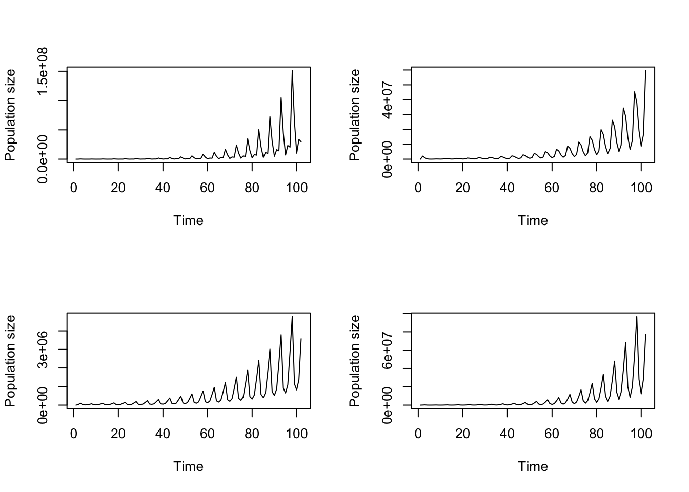
Figure 8.19: Bootstrapped function-based ahistorical projections of Cypripedium candidum
Voilà!
8.7 Points to remember
- Package
lefko3includes a number of functions to perform different styles of matrix projection.
- Function
projection3()is the quickest simulation tool for most situations, because it uses pre-defined matrices and so does not create matrices at every step.
- The greatest generality is available with function
f_projection3(), because it creates new matrices at every time step based on input vital rate models and user-defined conditions, including unique values of environmental or individual covariates.
- Projections can start with any particular population vector, and this can be set with the
start_inputandstart_frameoptions.
- Annual and individual covariates can be used to develop custom projection using environmental variables.
- Projections may be appended together with the
append_lP()function, provided that they share the same life history model as given in the associated stageframe.
- Bootstrapped projections are performed using the same functions, in combinations with the same methods as described for bootstrapped MPM creation.