Chapter 6 Matrix Models III: Age (Leslie), Hybrid Age, and Age-by-Stage MPMs
The really frightening thing about middle age is that you know you’ll grow out of it.
The first MPMs were age-classified, and are known as Leslie MPMs in honor of their creator (Leslie 1945). However, in many organisms, age is considered less important in determining demography than other variables. Stage-classified, or Lefkovitch, MPMs were developed with this in mind, and they allow the life history of an organism to be stratified by life history stages instead of age (Lefkovitch 1965). Life history stages can be defined as necessary by any status variable or combination of status variables (Caswell 2001), making the stage-based MPM a very flexible and powerful means to analyze population dynamics.
For much of the history of the MPM, the dichotomy between age-classified and stage-classified MPMs was strict and driven by the lack of computing power to analyze complex relationships in large matrices. With the advent of powerful home computers, more and more ecologists have addressed questions in population dynamics using age-by-stage MPMs, which are MPMs that incorporate both age and stage (Caswell & Salguero-Gómez 2013).
In this chapter, we will describe three kinds of age-classified MPMs, and how to build them using lefko3. They are as follows:
- Leslie MPMs: Purely age-classified; the simplest MPM to consider (section 6.5).
- Age-hybrid MPMs: Leslie MPMs with an extra stage that does not fit age-based conventions (section 6.6).
- Age-by-stage MPMs: MPMs built as block matrices with a stage-based design that is repeated across ages (section 6.2).
6.1 What are age-based, age-hybrid, and age-by-stage MPM?
We will begin with a short introduction to the core theory on age in MPMs. We strongly advise readers interested in this style of MPM to read Caswell et al. (2018), which is the most comprehensive overview of the theory behind age-by-stage MPMs that we are aware of.
Age-classified, or Leslie, MPMs treat the life history of an organism as a series of ages rather than stages. Each age can be thought of as a stage and is of equal duration. The number of ages to include is decided through demographic studies that attempt to determine which groups of ages have unique demographic characteristics. The only transitions that are possible are one-way survival transitions from one age to the next, survival transitions between the final age and itself if the lifespan has no hard limit, and fecundity from any reproductive age to age 0 (if post-breeding) or age 1 (if pre-breeding).
Let’s look at an example. Suppose that we are studying an organism that can live for potentially many years, such as an albatross or other long-lived seabird. We conduct several years of monitoring, and find that the seabird at our monitored population seems to follow a basic pattern in which survival is relatively low in the first year, higher in the second, and from the third year on survival is typically quite high and stable. Although the maximum longevity is unknown, nonetheless birds seem to live not much longer than 20 years. Fecundity occurs from the third year on, with the first two years spent as a juvenile. In this circumstance, we might develop a Leslie matrix with the following structure.
\[\begin{equation} \left[\begin{array} {rrr} 0 & 0 & F _{1,3} \\ S _{2,1} & 0 & 0 \\ 0 & S _{3,2} & S _{3,3} \\ \end{array}\right] \tag{6.1} \end{equation}\]
This matrix includes only three rows and columns. Survival-transition probabilities are typically just below the diagonal, and represent the probability of surviving from age \(i\) (column \(i\)) to age \(i+1\) (row \(i+1\)). There is a notable exception in element \(S _{3,3}\), which is the survival-transition probability for an organism to stay alive within the final age. We do not model further ages because our studies have suggested no predictable age-based change in vital rates beyond that age. Thus, this stasis transition allows us to model the tendency of organisms to live on without an explicit maximum longevity in a state in which the probability of survival is not expected to change. Fecundity is in the top row and final column (\(F_{1,3}\)), since all offspring begin in the first age.
Let’s now consider a more complicated scenario. Perhaps we have a similar life history in a plant, in which we have three core ages. However, we might wish to add a dormant seed stage, which allows the plant to survive as a dormant propagule that does not fit the age dynamics noted above. In that case, we might build an age-hybrid MPM, in which we simply add a stage as a new row and column to the matrix, as below.
\[\begin{equation} \left[\begin{array} {rrrr} S _{1,1} & 0 & 0 & F _{1,4} \\ S _{2,1} & 0 & 0 & F _{2,4} \\ 0 & S _{3,2} & 0 & 0 \\ 0 & 0 & S _{4,3} & S _{4,4} \\ \end{array}\right] \tag{6.2} \end{equation}\]
Note in the equation above that the first row and the first column are different, and there are now two fecundity paths reflecting the production of dormant seeds and seeds that germinate within a year of production. However, the rest of the MPM is the same as equation (6.1), except that the subscripts have been updated.
Finally, age-by-stage MPMs differ from the above because they incorporate both age and stage throughout, and so the matrix needs to be expanded to include both characteristics. The standard approach is to create block matrices in which each age has potentially several stages, and survival-transition probabilities must describe the probability of transitioning from each stage at one age to each stage in the next.
As an example, let’s take the three stage life history above, which has a single newborn stage and two adult stages, only one of which is reproductive. Let’s further assume that age impacts survival and fecundity only for the first four years, beyond which survival and fecundity transitions remain essentially the same. These conditions lead to the following age-by-stage matrix.
\[\begin{equation} \left[\begin{array} {rrrrrrr} 0 & 0 & F _{1A,2C} & 0 & F _{1A,3C} & 0 & F _{1A,4+C} \\ S _{2B,1A} & 0 & 0 & 0 & 0 & 0 & 0 \\ S _{2C,1A} & 0 & 0 & 0 & 0 & 0 & 0 \\ 0 & S _{3B,2B} & S _{3B,2C} & 0 & 0 & 0 & 0 \\ 0 & S _{3C,2B} & S _{3C,2C} & 0 & 0 & 0 & 0 \\ 0 & 0 & 0 & S _{4B,3B} & S _{4B,3C} & S _{5+B,4B} & S _{5+B,4+C} \\ 0 & 0 & 0 & S _{4C,3B} & S _{4C,3C} & S _{5+C,4B} & S _{5+C,4+C} \\ \end{array}\right] \tag{6.3} \end{equation}\]
Here, we have only one possible initial stage, followed by two possible stages in all later ages. Looking only at the columns, column 1 refers to age 1, which only includes the seedling stage; columns 2 and 3 refer to age 2, which includes non-reproductive and reproductive adult stages; columns 4 and 5 refer to age 3, which also includes non-reproductive and reproductive adult stages; and columns 6 and 7 refer to ages 4 and higher, once again also including non-reproductive and reproductive adult stages. While the columns refer to the From ages and stages (age and stage in time t), the rows refer to the To ages and stages (age and stage in time t+1), and are in the same order as the columns. If we ignore stage and consider only the placement of age-related transitions, then we see that we are still generally following the Leslie MPM pattern of placing survival-transition probabilities below the block-level diagonal for all but the final transitions. We also have more fecundity terms because although only one stage is reproductive, multiple reproductive ages occur, and all of these fecundity terms must stay within the first row (more entry rows are possible only if the life history of the organism can start from multiple different stages).
The above matrix is ahistorical. However, unlike a pure Leslie MPM, the possibility of different stages within each age allows for the estimation of historical age-by-stage MPMs. Package lefko3 does not support historical age-by-stage matrices.
6.2 Developing function-based age-by-stage MPMs
Package lefko3 can produce both raw (empirical) and function-based age-by-stage MPMs. Let’s start with the latter. For our example, we will use the lathyrus dataset that comes with lefko3 to illustrate the estimation of function-based age-by-stage MPMs. First, let’s load the dataset, and then look at its dimensions and a summary.
data(lathyrus)

dim(lathyrus)
> [1] 1119   38
summary(lathyrus)
>     SUBPLOT          GENET          Volume88         lnVol88
>  Min.   :1.000   Min.   :  1.0   Min.   :   3.4   Min.   :1.200
>  1st Qu.:2.000   1st Qu.: 48.0   1st Qu.:  63.0   1st Qu.:4.100
>  Median :3.000   Median : 97.0   Median : 732.5   Median :6.600
>  Mean   :3.223   Mean   :110.2   Mean   : 749.4   Mean   :5.538
>  3rd Qu.:4.000   3rd Qu.:167.5   3rd Qu.:1025.5   3rd Qu.:6.900
>  Max.   :6.000   Max.   :284.0   Max.   :7032.0   Max.   :8.900
>                                  NA's   :404      NA's   :404
>     FCODE88           Flow88       Intactseed88 Dead1988       Dormant1988
>  Min.   :0.0000   Min.   : 1.00   Min.   : 0    Mode:logical   Mode:logical
>  1st Qu.:0.0000   1st Qu.: 4.00   1st Qu.: 0    NA's:1119      NA's:1119
>  Median :0.0000   Median : 8.00   Median : 0
>  Mean   :0.3399   Mean   :11.86   Mean   : 3
>  3rd Qu.:1.0000   3rd Qu.:15.00   3rd Qu.: 4
>  Max.   :1.0000   Max.   :66.00   Max.   :34
>  NA's   :404      NA's   :910     NA's   :875
>  Missing1988     Seedling1988      Volume89         lnVol89
>  Mode:logical   Min.   :1.000   Min.   :   1.8   Min.   :0.600
>  NA's:1119      1st Qu.:2.000   1st Qu.:  15.6   1st Qu.:2.700
>                 Median :2.000   Median : 118.8   Median :4.800
>                 Mean   :2.144   Mean   : 573.3   Mean   :4.855
>                 3rd Qu.:3.000   3rd Qu.: 968.8   3rd Qu.:6.900
>                 Max.   :3.000   Max.   :6539.4   Max.   :8.800
>                 NA's   :1022    NA's   :294      NA's   :294
>     FCODE89           Flow89       Intactseed89       Dead1989
>  Min.   :0.0000   Min.   : 1.00   Min.   : 0.000   Min.   :1
>  1st Qu.:0.0000   1st Qu.: 5.00   1st Qu.: 0.000   1st Qu.:1
>  Median :0.0000   Median :11.00   Median : 5.000   Median :1
>  Mean   :0.2667   Mean   :14.88   Mean   : 8.273   Mean   :1
>  3rd Qu.:1.0000   3rd Qu.:20.00   3rd Qu.:13.000   3rd Qu.:1
>  Max.   :1.0000   Max.   :97.00   Max.   :66.000   Max.   :1
>  NA's   :294      NA's   :906     NA's   :899      NA's   :1077
>   Dormant1989    Missing1989    Seedling1989      Volume90         lnVol90
>  Min.   :1      Min.   :1      Min.   :1.000   Min.   :   2.1   Min.   :0.700
>  1st Qu.:1      1st Qu.:1      1st Qu.:2.000   1st Qu.:  12.6   1st Qu.:2.500
>  Median :1      Median :1      Median :2.000   Median :  61.0   Median :4.100
>  Mean   :1      Mean   :1      Mean   :2.136   Mean   : 244.1   Mean   :4.207
>  3rd Qu.:1      3rd Qu.:1      3rd Qu.:2.000   3rd Qu.: 295.2   3rd Qu.:5.700
>  Max.   :1      Max.   :1      Max.   :3.000   Max.   :4242.8   Max.   :8.400
>  NA's   :1046   NA's   :1112   NA's   :1001    NA's   :245      NA's   :245
>     FCODE90           Flow90        Intactseed90       Dead1990
>  Min.   :0.0000   Min.   : 1.000   Min.   : 0.000   Min.   :1
>  1st Qu.:0.0000   1st Qu.: 3.000   1st Qu.: 0.000   1st Qu.:1
>  Median :0.0000   Median : 6.000   Median : 0.000   Median :1
>  Mean   :0.1581   Mean   : 8.104   Mean   : 2.514   Mean   :1
>  3rd Qu.:0.0000   3rd Qu.:10.750   3rd Qu.: 1.000   3rd Qu.:1
>  Max.   :1.0000   Max.   :54.000   Max.   :37.000   Max.   :1
>  NA's   :246      NA's   :985      NA's   :981      NA's   :1007
>   Dormant1990    Missing1990    Seedling1990      Volume91         lnVol91
>  Min.   :1      Min.   :1      Min.   :1.000   Min.   :   4.0   Min.   :1.400
>  1st Qu.:1      1st Qu.:1      1st Qu.:2.000   1st Qu.:  12.0   1st Qu.:2.500
>  Median :1      Median :1      Median :2.000   Median : 118.5   Median :4.800
>  Mean   :1      Mean   :1      Mean   :2.186   Mean   : 418.7   Mean   :4.642
>  3rd Qu.:1      3rd Qu.:1      3rd Qu.:2.000   3rd Qu.: 689.7   3rd Qu.:6.500
>  Max.   :1      Max.   :1      Max.   :3.000   Max.   :6645.8   Max.   :8.800
>  NA's   :1054   NA's   :1105   NA's   :1049    NA's   :305      NA's   :305
>     FCODE91           Flow91       Intactseed91       Dead1991    Dormant1991
>  Min.   :0.0000   Min.   : 1.00   Min.   : 0.000   Min.   :1     Min.   :1
>  1st Qu.:0.0000   1st Qu.: 4.00   1st Qu.: 0.000   1st Qu.:1     1st Qu.:1
>  Median :0.0000   Median : 8.00   Median : 3.500   Median :1     Median :1
>  Mean   :0.2525   Mean   :11.12   Mean   : 5.805   Mean   :1     Mean   :1
>  3rd Qu.:1.0000   3rd Qu.:15.00   3rd Qu.:10.000   3rd Qu.:1     3rd Qu.:1
>  Max.   :1.0000   Max.   :48.00   Max.   :48.000   Max.   :1     Max.   :1
>  NA's   :307      NA's   :954     NA's   :919      NA's   :925   NA's   :1034
>   Missing1991    Seedling1991
>  Min.   :1      Min.   :1.000
>  1st Qu.:1      1st Qu.:2.000
>  Median :1      Median :2.000
>  Mean   :1      Mean   :1.973
>  3rd Qu.:1      3rd Qu.:2.000
>  Max.   :1      Max.   :3.000
>  NA's   :1095   NA's   :1082
This dataset includes information on 1119 individuals, so there are 1119 rows with data (not counting the header). There are 38 columns. The first two columns are variables identifying each individual (SUBPLOT refers to the patch, and GENET refers to individual identity), with each individual’s data entirely restricted to one row. This is followed by four sets of nine columns, each named VolumeXX, lnVolXX, FCODEXX, FlowXX, IntactseedXX, Dead19XX, DormantXX, Missing19XX, and SeedlingXX, where XX corresponds to the year of observation and with years organized consecutively. Thus, columns 3-11 refer to year 1988, columns 12-20 refer to year 1989, etc.
To begin, we will create a stageframe that describes the organism’s life cycle for this dataset. In this case, the life history model is the following life cycle graph (figure 6.1).
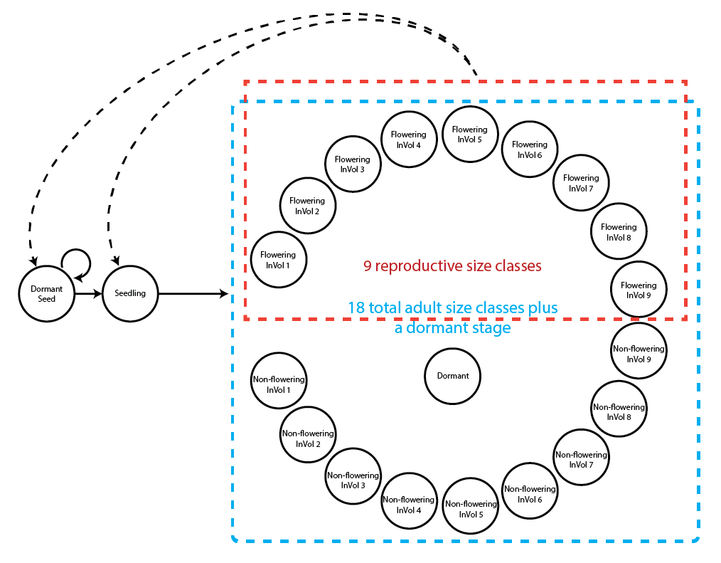
This model is based on the life history model provided in Ehrlén (2000), but we utilize a different size classification based on the natural logarithm of the leaf volume to make the size distribution more closely match a symmetric and somewhat normal distribution. This transformation can be justified biologically by viewing leaf volume allometrically.
Our stageframe needs to include complete descriptions of all stages that occur in the dataset, with each stage defined uniquely, and also needs to describe the ages for each stage portrayed in our life history model. Since this object can be used for automated classification of individuals, all sizes, reproductive states, and other characteristics defining each proper stage in the dataset need to be accounted for explicitly. This can be difficult if a few data points exist outside the range of sizes specified in the stageframe. Such points can cause problems, because rare stages can cause an overestimation of survival for existing stages under some circumstances, and can also yield spurious values for survival-transition probabilities and fecundity rates. The final description of each stage occurring in the dataset must also avoid complete overlap with any other stage also found in the dataset, although partial overlap is allowed and expected.
Before creating the stage frame, let’s explore the possible size variables. We will particularly look at summaries of the distribution of original and log sizes.
summary(c(lathyrus$Volume88, lathyrus$Volume89, lathyrus$Volume90,
    lathyrus$Volume91))
>    Min. 1st Qu.  Median    Mean 3rd Qu.    Max.    NA's
>     1.8    14.7   123.0   484.2   732.5  7032.0    1248
summary(c(lathyrus$lnVol88, lathyrus$lnVol89, lathyrus$lnVol90,
    lathyrus$lnVol91))
>    Min. 1st Qu.  Median    Mean 3rd Qu.    Max.    NA's
>   0.600   2.700   4.800   4.777   6.600   8.900    1248
The upper summary shows the original size, while the lower line shows the size given in logarithmic terms. We should note the size minima and maxima, because we have been using 0 as the size of vegetatively dormant individuals. The lowest raw size is 1.8, with a maximum of 7032.0. The minimum log size is 0.6, and the maximum is 8.9. Since the minimum raw size is above 0 (i.e. all log sizes should be positive), and since the number of NAs has not increased (increased NAs would suggest that some unusable log sizes occur in the dataset), we are able to use the log size value 0 as an indicator of vegetative dormancy. Note, however, that vegetative dormancy is also currently included in the many NAs that occur in size variables in this dataset.
It can also help to take a look at plots of these distributions. We will plot raw and log volume (figure 6.2).
par(mfrow=c(1,2))

plot(density(c(lathyrus$Volume88, lathyrus$Volume89, lathyrus$Volume90,
    lathyrus$Volume91), na.rm = TRUE), main = "", xlab = "Volume", bty = "n")
title("a)", adj = 0)

plot(density(c(lathyrus$lnVol88, lathyrus$lnVol89, lathyrus$lnVol90,
    lathyrus$lnVol91), na.rm = TRUE), main = "", xlab = "Log volume", bty = "n")
title("b)", adj = 0)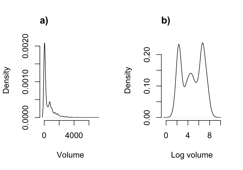
Figure 6.2: Density plot of aboveground plant volume (a) and log volume (b).
Note how highly skewed the raw volume distribution is. This might cause some difficulty if we use raw size untransformed and with a Gaussian distribution. Certainly, a gamma distribution might be justified, and users are urged to explore that approach. We will use the log volume here, which looks ‘better’ than the raw volume distribution in the sense that it is closer to some semblance of a Gaussian distribution, mostly through an increased level of symmetry. We can then assume that log volume is Gaussian-distributed and that the mean bears no relationship to the variance.
We will now develop a stageframe using log leaf volume in stage classification. We will build this by creating vectors of the values describing each stage, always in the same order. Because we wish to build an age-by-stage MPM, we will also incorporate age information for each stage. Here, we include minimum and maximum ages for each stage via the vectors minima and maxima (NA in the maximum age vector is interpreted as meaning that there is no maximum).
sizevector <- c(0, 4.6, 0, 1, 2, 3, 4, 5, 6, 7, 8, 9, 1, 2, 3, 4, 5, 6, 7, 8, 9)
stagevector <- c("Sd", "Sdl", "Dorm", "Sz1nr", "Sz2nr", "Sz3nr", "Sz4nr",
"Sz5nr","Sz6nr", "Sz7nr", "Sz8nr", "Sz9nr", "Sz1r", "Sz2r", "Sz3r", "Sz4r",
"Sz5r", "Sz6r", "Sz7r", "Sz8r", "Sz9r")
repvector <- c(0, 0, 0, 0, 0, 0, 0, 0, 0, 0, 0, 0, 1, 1, 1, 1, 1, 1, 1, 1, 1)
obsvector <- c(0, 1, 0, 1, 1, 1, 1, 1, 1, 1, 1, 1, 1, 1, 1, 1, 1, 1, 1, 1, 1)
matvector <- c(0, 0, 1, 1, 1, 1, 1, 1, 1, 1, 1, 1, 1, 1, 1, 1, 1, 1, 1, 1, 1)
immvector <- c(1, 1, 0, 0, 0, 0, 0, 0, 0, 0, 0, 0, 0, 0, 0, 0, 0, 0, 0, 0, 0)
propvector <- c(1, 0, 0, 0, 0, 0, 0, 0, 0, 0, 0, 0, 0, 0, 0, 0, 0, 0, 0, 0, 0)
indataset <- c(0, 1, 1, 1, 1, 1, 1, 1, 1, 1, 1, 1, 1, 1, 1, 1, 1, 1, 1, 1, 1)
binvec <- c(0, 4.6, 0.5, 0.5, 0.5, 0.5, 0.5, 0.5, 0.5, 0.5, 0.5, 0.5, 0.5, 0.5,
0.5, 0.5, 0.5, 0.5, 0.5, 0.5, 0.5)
minima <- c(1, 1, 2, 2, 2, 2, 2, 2, 2, 2, 2, 2, 2, 2, 2, 2, 2, 2, 2, 2, 2)
maxima <- c(NA, 1, NA, NA, NA, NA, NA, NA, NA, NA, NA, NA, NA, NA, NA, NA,
NA, NA, NA, NA, NA)
comments <- c("Dormant seed", "Seedling", "Dormant", "Size 1 Veg", "Size 2 Veg",
"Size 3 Veg", "Size 4 Veg", "Size 5 Veg", "Size 6 Veg", "Size 7 Veg",
"Size 8 Veg", "Size 9 Veg", "Size 1 Flo", "Size 2 Flo", "Size 3 Flo",
"Size 4 Flo", "Size 5 Flo", "Size 6 Flo", "Size 7 Flo", "Size 8 Flo",
"Size 9 Flo")
lathframeln <- sf_create(sizes = sizevector, stagenames = stagevector,
repstatus = repvector, obsstatus = obsvector, propstatus = propvector,
immstatus = immvector, matstatus = matvector, indataset = indataset,
binhalfwidth = binvec, minage = minima, maxage = maxima, comments = comments)
lathframeln
> stage size size_b size_c min_age max_age repstatus obsstatus propstatus
> 1 Sd 0.0 NA NA 1 NA 0 0 1
> 2 Sdl 4.6 NA NA 1 1 0 1 0
> 3 Dorm 0.0 NA NA 2 NA 0 0 0
> 4 Sz1nr 1.0 NA NA 2 NA 0 1 0
> 5 Sz2nr 2.0 NA NA 2 NA 0 1 0
> 6 Sz3nr 3.0 NA NA 2 NA 0 1 0
> 7 Sz4nr 4.0 NA NA 2 NA 0 1 0
> 8 Sz5nr 5.0 NA NA 2 NA 0 1 0
> 9 Sz6nr 6.0 NA NA 2 NA 0 1 0
> 10 Sz7nr 7.0 NA NA 2 NA 0 1 0
> 11 Sz8nr 8.0 NA NA 2 NA 0 1 0
> 12 Sz9nr 9.0 NA NA 2 NA 0 1 0
> 13 Sz1r 1.0 NA NA 2 NA 1 1 0
> 14 Sz2r 2.0 NA NA 2 NA 1 1 0
> 15 Sz3r 3.0 NA NA 2 NA 1 1 0
> 16 Sz4r 4.0 NA NA 2 NA 1 1 0
> 17 Sz5r 5.0 NA NA 2 NA 1 1 0
> 18 Sz6r 6.0 NA NA 2 NA 1 1 0
> 19 Sz7r 7.0 NA NA 2 NA 1 1 0
> 20 Sz8r 8.0 NA NA 2 NA 1 1 0
> 21 Sz9r 9.0 NA NA 2 NA 1 1 0
> immstatus matstatus indataset binhalfwidth_raw sizebin_min sizebin_max
> 1 1 0 0 0.0 0.0 0.0
> 2 1 0 1 4.6 0.0 9.2
> 3 0 1 1 0.5 -0.5 0.5
> 4 0 1 1 0.5 0.5 1.5
> 5 0 1 1 0.5 1.5 2.5
> 6 0 1 1 0.5 2.5 3.5
> 7 0 1 1 0.5 3.5 4.5
> 8 0 1 1 0.5 4.5 5.5
> 9 0 1 1 0.5 5.5 6.5
> 10 0 1 1 0.5 6.5 7.5
> 11 0 1 1 0.5 7.5 8.5
> 12 0 1 1 0.5 8.5 9.5
> 13 0 1 1 0.5 0.5 1.5
> 14 0 1 1 0.5 1.5 2.5
> 15 0 1 1 0.5 2.5 3.5
> 16 0 1 1 0.5 3.5 4.5
> 17 0 1 1 0.5 4.5 5.5
> 18 0 1 1 0.5 5.5 6.5
> 19 0 1 1 0.5 6.5 7.5
> 20 0 1 1 0.5 7.5 8.5
> 21 0 1 1 0.5 8.5 9.5
> sizebin_center sizebin_width binhalfwidthb_raw sizebinb_min sizebinb_max
> 1 0.0 0.0 NA NA NA
> 2 4.6 9.2 NA NA NA
> 3 0.0 1.0 NA NA NA
> 4 1.0 1.0 NA NA NA
> 5 2.0 1.0 NA NA NA
> 6 3.0 1.0 NA NA NA
> 7 4.0 1.0 NA NA NA
> 8 5.0 1.0 NA NA NA
> 9 6.0 1.0 NA NA NA
> 10 7.0 1.0 NA NA NA
> 11 8.0 1.0 NA NA NA
> 12 9.0 1.0 NA NA NA
> 13 1.0 1.0 NA NA NA
> 14 2.0 1.0 NA NA NA
> 15 3.0 1.0 NA NA NA
> 16 4.0 1.0 NA NA NA
> 17 5.0 1.0 NA NA NA
> 18 6.0 1.0 NA NA NA
> 19 7.0 1.0 NA NA NA
> 20 8.0 1.0 NA NA NA
> 21 9.0 1.0 NA NA NA
> sizebinb_center sizebinb_width binhalfwidthc_raw sizebinc_min sizebinc_max
> 1 NA NA NA NA NA
> 2 NA NA NA NA NA
> 3 NA NA NA NA NA
> 4 NA NA NA NA NA
> 5 NA NA NA NA NA
> 6 NA NA NA NA NA
> 7 NA NA NA NA NA
> 8 NA NA NA NA NA
> 9 NA NA NA NA NA
> 10 NA NA NA NA NA
> 11 NA NA NA NA NA
> 12 NA NA NA NA NA
> 13 NA NA NA NA NA
> 14 NA NA NA NA NA
> 15 NA NA NA NA NA
> 16 NA NA NA NA NA
> 17 NA NA NA NA NA
> 18 NA NA NA NA NA
> 19 NA NA NA NA NA
> 20 NA NA NA NA NA
> 21 NA NA NA NA NA
> sizebinc_center sizebinc_width group comments
> 1 NA NA 0 Dormant seed
> 2 NA NA 0 Seedling
> 3 NA NA 0 Dormant
> 4 NA NA 0 Size 1 Veg
> 5 NA NA 0 Size 2 Veg
> 6 NA NA 0 Size 3 Veg
> 7 NA NA 0 Size 4 Veg
> 8 NA NA 0 Size 5 Veg
> 9 NA NA 0 Size 6 Veg
> 10 NA NA 0 Size 7 Veg
> 11 NA NA 0 Size 8 Veg
> 12 NA NA 0 Size 9 Veg
> 13 NA NA 0 Size 1 Flo
> 14 NA NA 0 Size 2 Flo
> 15 NA NA 0 Size 3 Flo
> 16 NA NA 0 Size 4 Flo
> 17 NA NA 0 Size 5 Flo
> 18 NA NA 0 Size 6 Flo
> 19 NA NA 0 Size 7 Flo
> 20 NA NA 0 Size 8 Flo
> 21 NA NA 0 Size 9 Flo
Once the stageframe is created, we can reorganize the dataset into historically-formatted vertical (hfv) format. Before doing this, we need to alter the dataset slightly. Currently, the variable GENET lists the individual number, but only within each subpopulation. We wish to identify each individual within each subpopulation uniquely, and this requires us to develop a new ID variable. For this purpose, we will create a new variable that concatenates the subpopulation and genet number together into one string, as below.
Now let’s use verticalize3(), which creates historically-formatted vertical datasets, as below. We will also replace NAs in size and fecundity variables with zeros for modelsearch to work properly when we build models of vital rates, so we will now set NAas0 = TRUE. Some care needs to be taken with this last step, since some authors give missing values extra meaning not present in a value of zero. In our case, a missing value indicates that a plant was dead (both size and fecundity are missing), was alive but not sprouting (size was missing), or was alive but did not produce seed (fecundity was missing). In all cases, these NA values may be replaced by zero, because other variables indicate those conditions.
We also have two choices for use as our reproductive status and fecundity variables. The first choice, FCODE88 indicates whether a plant flowered. The second choice, Intactseed88, indicates the number of seed produced. The choice of which to use depends strongly on the life history model. In our case, we would like to treat all plants that flowered as reproductive, but treat fecundity in terms of real seed produced. The reason is that we believe that flowering plants have a different demography than non-flowering plants, either reflecting reproductive costs, or, conversely, because flowering plants might have more resources and hence higher survival than non-flowering plants, and so we wish to separate transitions among these two groups. So, let’s use FCODE88 to indicate reproductive status, and Intactseed88 to indicate fecundity. Once complete, we will look at a summary.
Finally, note that in the input to the following function, we utilize a strictly repeating pattern of variable names arranged in the same order for each monitoring occasion. This arrangement allows us to enter only the first variable in each set, as long as noyears and blocksize are set properly and no gaps or shuffles appear in the dataset. The data management functions that we have created for lefko3 do not require such repeating patterns, but they do make the required input in the function much shorter and more succinct.
lathvertln <- verticalize3(lathyrus, noyears = 4, firstyear = 1988,
  patchidcol = "SUBPLOT", individcol = "indiv_id", blocksize = 9,
  juvcol = "Seedling1988", sizeacol = "lnVol88", repstracol = "FCODE88",
  fecacol = "Intactseed88", deadacol = "Dead1988", nonobsacol = "Dormant1988",
  stageassign = lathframeln, stagesize = "sizea", censorcol = "Missing1988",
  censorkeep = NA, censorRepeat = TRUE, NAas0 = TRUE, censor = TRUE)

summary_hfv(lathvertln, full = TRUE)
>
> This hfv dataset contains 2527 rows, 54 variables, 1 population,
> 6 patches, 1053 individuals, and 3 time steps.
>      rowid           popid              patchid        individ
>  Min.   :   1.0   Length:2527        Min.   :1.000   Length:2527
>  1st Qu.: 237.0   Class :character   1st Qu.:1.000   Class :character
>  Median : 522.0   Mode  :character   Median :3.000   Mode  :character
>  Mean   : 537.3                      Mean   :3.195
>  3rd Qu.: 820.5                      3rd Qu.:4.000
>  Max.   :1118.0                      Max.   :6.000
>      year2        firstseen       lastseen        obsage       obslifespan
>  Min.   :1988   Min.   :   0   Min.   :   0   Min.   :1.000   Min.   :0.000
>  1st Qu.:1988   1st Qu.:1988   1st Qu.:1991   1st Qu.:1.000   1st Qu.:2.000
>  Median :1989   Median :1988   Median :1991   Median :2.000   Median :3.000
>  Mean   :1989   Mean   :1979   Mean   :1981   Mean   :1.822   Mean   :2.437
>  3rd Qu.:1990   3rd Qu.:1988   3rd Qu.:1991   3rd Qu.:2.000   3rd Qu.:3.000
>  Max.   :1990   Max.   :1990   Max.   :1991   Max.   :3.000   Max.   :3.000
>      sizea1        size1added       repstra1       repstr1added
>  Min.   :0.000   Min.   :0.000   Min.   :0.0000   Min.   :0.0000
>  1st Qu.:0.000   1st Qu.:0.000   1st Qu.:0.0000   1st Qu.:0.0000
>  Median :2.200   Median :2.200   Median :0.0000   Median :0.0000
>  Mean   :2.957   Mean   :2.957   Mean   :0.1805   Mean   :0.1805
>  3rd Qu.:6.400   3rd Qu.:6.400   3rd Qu.:0.0000   3rd Qu.:0.0000
>  Max.   :8.900   Max.   :8.900   Max.   :1.0000   Max.   :1.0000
>      feca1          fec1added         censor1    juvgiven1
>  Min.   : 0.000   Min.   : 0.000   Min.   :0   Min.   :0.00000
>  1st Qu.: 0.000   1st Qu.: 0.000   1st Qu.:0   1st Qu.:0.00000
>  Median : 0.000   Median : 0.000   Median :0   Median :0.00000
>  Mean   : 0.989   Mean   : 0.989   Mean   :0   Mean   :0.06292
>  3rd Qu.: 0.000   3rd Qu.: 0.000   3rd Qu.:0   3rd Qu.:0.00000
>  Max.   :66.000   Max.   :66.000   Max.   :0   Max.   :1.00000
>    obsstatus1       repstatus1       fecstatus1        matstatus1
>  Min.   :0.0000   Min.   :0.0000   Min.   :0.00000   Min.   :0.0000
>  1st Qu.:0.0000   1st Qu.:0.0000   1st Qu.:0.00000   1st Qu.:0.0000
>  Median :1.0000   Median :0.0000   Median :0.00000   Median :1.0000
>  Mean   :0.5548   Mean   :0.1805   Mean   :0.08983   Mean   :0.5204
>  3rd Qu.:1.0000   3rd Qu.:0.0000   3rd Qu.:0.00000   3rd Qu.:1.0000
>  Max.   :1.0000   Max.   :1.0000   Max.   :1.00000   Max.   :1.0000
>      alive1          stage1           stage1index         sizea2
>  Min.   :0.0000   Length:2527        Min.   : 0.000   Min.   :0.000
>  1st Qu.:0.0000   Class :character   1st Qu.: 0.000   1st Qu.:2.500
>  Median :1.0000   Mode  :character   Median : 3.000   Median :4.700
>  Mean   :0.5833                      Mean   : 6.137   Mean   :4.565
>  3rd Qu.:1.0000                      3rd Qu.:10.000   3rd Qu.:6.600
>  Max.   :1.0000                      Max.   :21.000   Max.   :8.900
>    size2added       repstra2      repstr2added       feca2
>  Min.   :0.000   Min.   :0.000   Min.   :0.000   Min.   : 0.00
>  1st Qu.:2.500   1st Qu.:0.000   1st Qu.:0.000   1st Qu.: 0.00
>  Median :4.700   Median :0.000   Median :0.000   Median : 0.00
>  Mean   :4.565   Mean   :0.237   Mean   :0.237   Mean   : 1.14
>  3rd Qu.:6.600   3rd Qu.:0.000   3rd Qu.:0.000   3rd Qu.: 0.00
>  Max.   :8.900   Max.   :1.000   Max.   :1.000   Max.   :66.00
>    fec2added        censor2    juvgiven2        obsstatus2       repstatus2
>  Min.   : 0.00   Min.   :0   Min.   :0.0000   Min.   :0.0000   Min.   :0.000
>  1st Qu.: 0.00   1st Qu.:0   1st Qu.:0.0000   1st Qu.:1.0000   1st Qu.:0.000
>  Median : 0.00   Median :0   Median :0.0000   Median :1.0000   Median :0.000
>  Mean   : 1.14   Mean   :0   Mean   :0.1112   Mean   :0.9454   Mean   :0.237
>  3rd Qu.: 0.00   3rd Qu.:0   3rd Qu.:0.0000   3rd Qu.:1.0000   3rd Qu.:0.000
>  Max.   :66.00   Max.   :0   Max.   :1.0000   Max.   :1.0000   Max.   :1.000
>    fecstatus2       matstatus2         alive2     stage2
>  Min.   :0.0000   Min.   :0.0000   Min.   :1   Length:2527
>  1st Qu.:0.0000   1st Qu.:1.0000   1st Qu.:1   Class :character
>  Median :0.0000   Median :1.0000   Median :1   Mode  :character
>  Mean   :0.1053   Mean   :0.8888   Mean   :1
>  3rd Qu.:0.0000   3rd Qu.:1.0000   3rd Qu.:1
>  Max.   :1.0000   Max.   :1.0000   Max.   :1
>   stage2index         sizea3        size3added       repstra3
>  Min.   : 2.000   Min.   :0.000   Min.   :0.000   Min.   :0.000
>  1st Qu.: 5.000   1st Qu.:2.300   1st Qu.:2.300   1st Qu.:0.000
>  Median : 8.000   Median :4.300   Median :4.300   Median :0.000
>  Mean   : 9.323   Mean   :4.043   Mean   :4.043   Mean   :0.218
>  3rd Qu.:10.000   3rd Qu.:6.300   3rd Qu.:6.300   3rd Qu.:0.000
>  Max.   :21.000   Max.   :8.800   Max.   :8.800   Max.   :1.000
>   repstr3added       feca3         fec3added        censor3    juvgiven3
>  Min.   :0.000   Min.   : 0.00   Min.   : 0.00   Min.   :0   Min.   :0
>  1st Qu.:0.000   1st Qu.: 0.00   1st Qu.: 0.00   1st Qu.:0   1st Qu.:0
>  Median :0.000   Median : 0.00   Median : 0.00   Median :0   Median :0
>  Mean   :0.218   Mean   : 1.29   Mean   : 1.29   Mean   :0   Mean   :0
>  3rd Qu.:0.000   3rd Qu.: 0.00   3rd Qu.: 0.00   3rd Qu.:0   3rd Qu.:0
>  Max.   :1.000   Max.   :66.00   Max.   :66.00   Max.   :0   Max.   :0
>    obsstatus3       repstatus3      fecstatus3       matstatus3
>  Min.   :0.0000   Min.   :0.000   Min.   :0.0000   Min.   :1
>  1st Qu.:1.0000   1st Qu.:0.000   1st Qu.:0.0000   1st Qu.:1
>  Median :1.0000   Median :0.000   Median :0.0000   Median :1
>  Mean   :0.8346   Mean   :0.218   Mean   :0.1116   Mean   :1
>  3rd Qu.:1.0000   3rd Qu.:0.000   3rd Qu.:0.0000   3rd Qu.:1
>  Max.   :1.0000   Max.   :1.000   Max.   :1.0000   Max.   :1
>      alive3          stage3           stage3index
>  Min.   :0.0000   Length:2527        Min.   : 0.000
>  1st Qu.:1.0000   Class :character   1st Qu.: 5.000
>  Median :1.0000   Mode  :character   Median : 7.000
>  Mean   :0.9224                      Mean   : 8.717
>  3rd Qu.:1.0000                      3rd Qu.:10.000
>  Max.   :1.0000                      Max.   :21.000
This dataset has 2527 rows representing our original dataset of over 1000 individuals. Ordinarily, we would now go on to produce vital rate models to create function-based MPMs. However, the fact that we are incorporating age in our analysis leads to the problem that there are many individuals in our dataset that are of unknown age. Lathyrus is a long-lived plant, and this demographic study lasted only four years, leading to a poor understanding of the ages of most plants. The hfv dataset that we have created includes an estimated age for each individual in each year, but this is estimated from the time in which the individual is first seen. Many individuals are first seen in the first year of the study, by which time many could have already been alive for several years. So, we will subset our data to eliminate individuals first seen in the very first year of the study.
lathvertln_small <- subset(lathvertln, firstseen > 1988)
summary_hfv(lathvertln_small, full = TRUE)
>
> This hfv dataset contains 531 rows, 54 variables, 1 population,
> 6 patches, 345 individuals, and 2 time steps.
>      rowid           popid              patchid        individ
>  Min.   :  30.0   Length:531         Min.   :1.000   Length:531
>  1st Qu.: 301.0   Class :character   1st Qu.:2.000   Class :character
>  Median : 582.0   Mode  :character   Median :3.000   Mode  :character
>  Mean   : 585.3                      Mean   :3.077
>  3rd Qu.: 800.5                      3rd Qu.:4.000
>  Max.   :1097.0                      Max.   :6.000
>      year2        firstseen       lastseen        obsage      obslifespan
>  Min.   :1989   Min.   :1989   Min.   :1989   Min.   :1.00   Min.   :0.000
>  1st Qu.:1989   1st Qu.:1989   1st Qu.:1990   1st Qu.:1.00   1st Qu.:1.000
>  Median :1990   Median :1989   Median :1991   Median :1.00   Median :2.000
>  Mean   :1990   Mean   :1989   Mean   :1991   Mean   :1.35   Mean   :1.367
>  3rd Qu.:1990   3rd Qu.:1989   3rd Qu.:1991   3rd Qu.:2.00   3rd Qu.:2.000
>  Max.   :1990   Max.   :1990   Max.   :1991   Max.   :2.00   Max.   :2.000
>      sizea1        size1added       repstra1        repstr1added
>  Min.   :0.000   Min.   :0.000   Min.   :0.00000   Min.   :0.00000
>  1st Qu.:0.000   1st Qu.:0.000   1st Qu.:0.00000   1st Qu.:0.00000
>  Median :0.000   Median :0.000   Median :0.00000   Median :0.00000
>  Mean   :1.175   Mean   :1.175   Mean   :0.02072   Mean   :0.02072
>  3rd Qu.:2.200   3rd Qu.:2.200   3rd Qu.:0.00000   3rd Qu.:0.00000
>  Max.   :8.400   Max.   :8.400   Max.   :1.00000   Max.   :1.00000
>      feca1           fec1added          censor1    juvgiven1
>  Min.   : 0.0000   Min.   : 0.0000   Min.   :0   Min.   :0.000
>  1st Qu.: 0.0000   1st Qu.: 0.0000   1st Qu.:0   1st Qu.:0.000
>  Median : 0.0000   Median : 0.0000   Median :0   Median :0.000
>  Mean   : 0.1243   Mean   : 0.1243   Mean   :0   Mean   :0.162
>  3rd Qu.: 0.0000   3rd Qu.: 0.0000   3rd Qu.:0   3rd Qu.:0.000
>  Max.   :34.0000   Max.   :34.0000   Max.   :0   Max.   :1.000
>    obsstatus1       repstatus1        fecstatus1        matstatus1
>  Min.   :0.0000   Min.   :0.00000   Min.   :0.00000   Min.   :0.0000
>  1st Qu.:0.0000   1st Qu.:0.00000   1st Qu.:0.00000   1st Qu.:0.0000
>  Median :0.0000   Median :0.00000   Median :0.00000   Median :0.0000
>  Mean   :0.3503   Mean   :0.02072   Mean   :0.01318   Mean   :0.1883
>  3rd Qu.:1.0000   3rd Qu.:0.00000   3rd Qu.:0.00000   3rd Qu.:0.0000
>  Max.   :1.0000   Max.   :1.00000   Max.   :1.00000   Max.   :1.0000
>      alive1          stage1           stage1index         sizea2
>  Min.   :0.0000   Length:531         Min.   : 0.000   Min.   :0.000
>  1st Qu.:0.0000   Class :character   1st Qu.: 0.000   1st Qu.:2.200
>  Median :0.0000   Mode  :character   Median : 0.000   Median :2.500
>  Mean   :0.3503                      Mean   : 1.881   Mean   :3.072
>  3rd Qu.:1.0000                      3rd Qu.: 2.000   3rd Qu.:3.600
>  Max.   :1.0000                      Max.   :20.000   Max.   :8.400
>    size2added       repstra2        repstr2added         feca2
>  Min.   :0.000   Min.   :0.00000   Min.   :0.00000   Min.   : 0.000
>  1st Qu.:2.200   1st Qu.:0.00000   1st Qu.:0.00000   1st Qu.: 0.000
>  Median :2.500   Median :0.00000   Median :0.00000   Median : 0.000
>  Mean   :3.072   Mean   :0.03578   Mean   :0.03578   Mean   : 0.145
>  3rd Qu.:3.600   3rd Qu.:0.00000   3rd Qu.:0.00000   3rd Qu.: 0.000
>  Max.   :8.400   Max.   :1.00000   Max.   :1.00000   Max.   :34.000
>    fec2added         censor2    juvgiven2        obsstatus2
>  Min.   : 0.000   Min.   :0   Min.   :0.0000   Min.   :0.0000
>  1st Qu.: 0.000   1st Qu.:0   1st Qu.:0.0000   1st Qu.:1.0000
>  Median : 0.000   Median :0   Median :0.0000   Median :1.0000
>  Mean   : 0.145   Mean   :0   Mean   :0.3465   Mean   :0.9849
>  3rd Qu.: 0.000   3rd Qu.:0   3rd Qu.:1.0000   3rd Qu.:1.0000
>  Max.   :34.000   Max.   :0   Max.   :1.0000   Max.   :1.0000
>    repstatus2        fecstatus2        matstatus2         alive2
>  Min.   :0.00000   Min.   :0.00000   Min.   :0.0000   Min.   :1
>  1st Qu.:0.00000   1st Qu.:0.00000   1st Qu.:0.0000   1st Qu.:1
>  Median :0.00000   Median :0.00000   Median :1.0000   Median :1
>  Mean   :0.03578   Mean   :0.01695   Mean   :0.6535   Mean   :1
>  3rd Qu.:0.00000   3rd Qu.:0.00000   3rd Qu.:1.0000   3rd Qu.:1
>  Max.   :1.00000   Max.   :1.00000   Max.   :1.0000   Max.   :1
>     stage2           stage2index         sizea3        size3added
>  Length:531         Min.   : 2.000   Min.   :0.000   Min.   :0.000
>  Class :character   1st Qu.: 2.000   1st Qu.:0.000   1st Qu.:0.000
>  Mode  :character   Median : 5.000   Median :2.400   Median :2.400
>                     Mean   : 5.209   Mean   :2.351   Mean   :2.351
>                     3rd Qu.: 7.000   3rd Qu.:3.200   3rd Qu.:3.200
>                     Max.   :20.000   Max.   :8.800   Max.   :8.800
>     repstra3        repstr3added         feca3           fec3added
>  Min.   :0.00000   Min.   :0.00000   Min.   : 0.0000   Min.   : 0.0000
>  1st Qu.:0.00000   1st Qu.:0.00000   1st Qu.: 0.0000   1st Qu.: 0.0000
>  Median :0.00000   Median :0.00000   Median : 0.0000   Median : 0.0000
>  Mean   :0.04143   Mean   :0.04143   Mean   : 0.2505   Mean   : 0.2505
>  3rd Qu.:0.00000   3rd Qu.:0.00000   3rd Qu.: 0.0000   3rd Qu.: 0.0000
>  Max.   :1.00000   Max.   :1.00000   Max.   :48.0000   Max.   :48.0000
>     censor3    juvgiven3   obsstatus3       repstatus3        fecstatus3
>  Min.   :0   Min.   :0   Min.   :0.0000   Min.   :0.00000   Min.   :0.00000
>  1st Qu.:0   1st Qu.:0   1st Qu.:0.0000   1st Qu.:0.00000   1st Qu.:0.00000
>  Median :0   Median :0   Median :1.0000   Median :0.00000   Median :0.00000
>  Mean   :0   Mean   :0   Mean   :0.7458   Mean   :0.04143   Mean   :0.01318
>  3rd Qu.:0   3rd Qu.:0   3rd Qu.:1.0000   3rd Qu.:0.00000   3rd Qu.:0.00000
>  Max.   :0   Max.   :0   Max.   :1.0000   Max.   :1.00000   Max.   :1.00000
>    matstatus3     alive3          stage3           stage3index
>  Min.   :1    Min.   :0.0000   Length:531         Min.   : 0.00
>  1st Qu.:1    1st Qu.:1.0000   Class :character   1st Qu.: 3.00
>  Median :1    Median :1.0000   Mode  :character   Median : 5.00
>  Mean   :1    Mean   :0.8117                      Mean   : 5.06
>  3rd Qu.:1    3rd Qu.:1.0000                      3rd Qu.: 6.00
>  Max.   :1    Max.   :1.0000                      Max.   :21.00
We are now down to only 531 rows and 345 individuals, so we have lost roughly 80% of the transition data here. That is a steep price to pay for accurate inference, but it is necessary in this case.
Let’s look at fecundity. Fecundity is integer-based, suggesting that it can be treated as a count variable. This package currently allows eight choices of count distributions: Gaussian, gamma, Poisson, negative binomial, zero-inflated Poisson, zero-inflated negative binomial, zero-truncated Poisson, and zero-truncated negative binomial. To assess which to use, we should first assess whether the mean and variance of the count are equal using a dispersion test. This test allows us to test whether the variance is greater than that expected under our mean value for fecundity, using a \(\chi ^2\) test. If it is not significantly different, then we may use some variant of the Poisson distribution. If the data are overdispersed, then we should use the negative binomial distribution. We should also test whether the number of zeros is more than expected under these distributions, and make the distribution zero-inflated if so. Note that, because we have not excluded 0s from fecundity using reproductive status, we should not use a zero-truncated distribution.
Let’s start off by looking at a bar plot of the distribution of fecundity (figure 6.3).
hist(subset(lathvertln_small, repstatus2 == 1)$feca2, breaks = 35,
  main = "Fecundity", xlab = "Intact seeds produced in occasion t")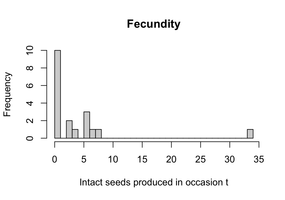
Figure 6.3: Histogram of fecundity in occasion t
We see that the distribution conforms to a classic count variable with a very low mean value. The first bar suggests that there may be too many zeros, as well. Let’s now formally test our assumptions, that the mean equals the variance and that the number of zeros meets expectation. Both tests use \(\chi ^2\) distribution-based approaches, with the zero-inflation test in particular based on Broek (1995). We will do this through a quality control assessment of the entire dataset for modeling, using hfv_qc(), into which we need to specify which vital rates we intend to model later, and the names of some key variables.
hfv_qc(lathvertln_small, indiv = "individ", year = "year2", age = "obsage",
  vitalrates = c("surv", "obs", "size", "repst", "fec"))
> Survival:
>
>   Data subset has 54 variables and 531 transitions.
>
>   Variable alive3 has 0 missing values.
>   Variable alive3 is a binomial variable.
>
>   Numbers of categories in data subset in possible random variables:
>   indiv id: 345   (singleton categories: 159)
>   year2: 2   (singleton categories: 0)
>
> Observation status:
>
>   Data subset has 54 variables and 431 transitions.
>
>   Variable obsstatus3 has 0 missing values.
>   Variable obsstatus3 is a binomial variable.
>
>   Numbers of categories in data subset in possible random variables:
>   indiv id: 281   (singleton categories: 131)
>   year2: 2   (singleton categories: 0)
>
> Primary size:
>
>   Data subset has 54 variables and 396 transitions.
>
>   Variable sizea3 has 0 missing values.
>   Variable sizea3 appears to be a floating point variable.
>   379 elements are not integers.
>   The minimum value of sizea3 is 0.7 and the maximum is 8.8.
>   The mean value of sizea3 is 3.153 and the variance is 1.818.
>   The value of the Shapiro-Wilk test of normality is 0.8367 with P = 8.608e-20.
>   Variable sizea3 differs significantly from a Gaussian distribution.
>
>   Variable sizea3 is fully positive, lacking even 0s.
>
>   Numbers of categories in data subset in possible random variables:
>   indiv id: 268   (singleton categories: 140)
>   year2: 2   (singleton categories: 0)
>
> Reproductive status:
>
>   Data subset has 54 variables and 396 transitions.
>
>   Variable repstatus3 has 0 missing values.
>   Variable repstatus3 is a binomial variable.
>
>   Numbers of categories in data subset in possible random variables:
>   indiv id: 268   (singleton categories: 140)
>   year2: 2   (singleton categories: 0)
>
> Fecundity:
>
>   Data subset has 54 variables and 19 transitions.
>
>   Variable feca2 has 0 missing values.
>   Variable feca2 appears to be an integer variable.
>
>   Variable feca2 is fully non-negative.
>
>   Overdispersion test:
>     Mean feca2 is 4.053
>     The variance in feca2 is 61.05
>     The probability of this dispersion level by chance assuming that
>     the true mean feca2 = variance in feca2,
>     and an alternative hypothesis of overdispersion, is 8.249e-152
>     Variable feca2 is significantly overdispersed.
>
>   Zero-inflation and truncation tests:
>     Mean lambda in feca2 is 0.01738
>     The actual number of 0s in feca2 is 10
>     The expected number of 0s in feca2 under the null hypothesis is 0.3302
>     The probability of this deviation in 0s from expectation by chance is 1.719e-69
>     Variable feca2 is significantly zero-inflated.
>
>   Numbers of categories in data subset in possible random variables:
>   indiv id: 16   (singleton categories: 13)
>   year2: 2   (singleton categories: 0)
We see that fecundity is significantly overdispersed, and has a significant excess of zeros. It is also a very small subset with only 19 data points. So, we should use a zero-inflated negative binomial distribution here, but we should note that the small size of the dataset may make good inference impossible and may justify simpler approaches. Note that our output also suggests problems with using the Gaussian distribution for size, but we will ignore that at this time.
Next, let’s create an ahistorical supplement table organizing the extra data that we need to incorporate into our matrices. Each row refers to a specific transition. The first two of these transitions are set to specific probabilities, which are the probabilities of germination and seed dormancy, estimated from a separate study. The final two terms are fecundity multipliers, which mark which transitions correspond to fecundity and provide information on what multiple of fecundity estimated via linear modeling applies to each case. Note that we can also include proxy transitions, in which we define a specific transition as being equal to another in the matrix. The latter approach is useful when some transitions cannot be estimated given a particular dataset, and so need to be set to other, proxy values that are estimable.
lathsupp2 <- supplemental(stage3 = c("Sd", "Sdl", "Sd", "Sdl"),
  stage2 = c("Sd", "Sd", "rep", "rep"), givenrate = c(0.345, 0.054, NA, NA),
  multiplier = c(NA, NA, 0.345, 0.054), type = c(1, 1, 3, 3),
  stageframe = lathframeln, historical = FALSE, stagebased = TRUE,
  agebased = TRUE)
> Warning: NA values in argument multiplier will be treated as 1 values.

lathsupp2
>   stage3 stage2 stage1 age2 eststage3 eststage2 eststage1 estage2 givenrate
> 1     Sd     Sd   <NA>   NA      <NA>      <NA>      <NA>      NA     0.345
> 2    Sdl     Sd   <NA>   NA      <NA>      <NA>      <NA>      NA     0.054
> 3     Sd    rep   <NA>   NA      <NA>      <NA>      <NA>      NA        NA
> 4    Sdl    rep   <NA>   NA      <NA>      <NA>      <NA>      NA        NA
>   offset multiplier convtype convtype_t12
> 1     NA      1.000        1            1
> 2     NA      1.000        1            1
> 3     NA      0.345        3            1
> 4     NA      0.054        3            1
Next we will run modelsearch() with the new vertical dataset. This function will develop our best-fit vital rate models for us. This function looks simple, but it automates several crucial and complex tasks in MPM analysis. Specifically, it automates 1) the building of global models for each vital rate requested, 2) the exhaustive construction of all reduced models, and 3) the selection of the best-fit models. In relation to our previous uses of this function in chapter 5, the most noteworthy difference is the inclusion of an age term (age = "obsage", which we know from looking at the summary of the vertical dataset). We will develop the full effects models here, which include main effects and all two-way interactions between age and other terms, including size and reproductive status. Note that we include age = "obsage", which tells modelsearch() what the name of the age variable is in our dataset, and test.age = TRUE, which tells the function to include the term in the global model of each vital rate.
Let’s start off by generating a set of vital rate models that covers the entire population.
lathmodelsln2 <- modelsearch(lathvertln_small, historical = FALSE,
  approach = "mixed", suite = "full", bestfit = "AICc&k", juvestimate = "Sdl",
  vitalrates = c("surv", "obs", "size", "repst", "fec"), sizedist = "gaussian",
  fecdist = "negbin", indiv = "individ", year = "year2", age = "obsage",
  year.as.random = TRUE, patch.as.random = TRUE, show.model.tables = TRUE,
  fec.zero = TRUE, test.age = TRUE, quiet = "partial")
Let’s see a summary of the lefkoMod object that we have created.
summary(lathmodelsln2)
> This LefkoMod object includes 8 linear models.
> Best-fit model criterion used: aicc&k
>
>
>
> Survival model:
> Generalized linear mixed model fit by maximum likelihood (Laplace
>   Approximation) [glmerMod]
>  Family: binomial  ( logit )
> Formula: alive3 ~ obsage + (1 | year2) + (1 | individ)
>    Data: surv.data
>       AIC       BIC    logLik -2*log(L)  df.resid
>  182.9812  198.3785  -87.4906  174.9812       343
> Random effects:
>  Groups  Name        Std.Dev.
>  individ (Intercept) 62.23
>  year2   (Intercept)  0.00
> Number of obs: 347, groups:  individ, 247; year2, 2
> Fixed Effects:
> (Intercept)       obsage
>       39.46       -13.65
> optimizer (Nelder_Mead) convergence code: 0 (OK) ; 0 optimizer warnings; 1 lme4 warnings
>
>
>
> Observation model:
> Generalized linear mixed model fit by maximum likelihood (Laplace
>   Approximation) [glmerMod]
>  Family: binomial  ( logit )
> Formula: obsstatus3 ~ sizea2 + (1 | year2) + (1 | individ)
>    Data: obs.data
>       AIC       BIC    logLik -2*log(L)  df.resid
>  184.0111  198.7454  -88.0055  176.0111       290
> Random effects:
>  Groups  Name        Std.Dev.
>  individ (Intercept) 1.107e-05
>  year2   (Intercept) 4.163e-01
> Number of obs: 294, groups:  individ, 203; year2, 2
> Fixed Effects:
> (Intercept)       sizea2
>      3.9774      -0.3997
> optimizer (Nelder_Mead) convergence code: 0 (OK) ; 0 optimizer warnings; 1 lme4 warnings
>
>
>
> Size model:
> Linear mixed model fit by REML ['lmerMod']
> Formula: sizea3 ~ sizea2 + (1 | year2) + (1 | individ)
>    Data: size.data
> REML criterion at convergence: 700.2483
> Random effects:
>  Groups   Name        Std.Dev.
>  individ  (Intercept) 0.0000
>  year2    (Intercept) 0.4826
>  Residual             0.8850
> Number of obs: 266, groups:  individ, 191; year2, 2
> Fixed Effects:
> (Intercept)       sizea2
>      0.7088       0.7777
> optimizer (nloptwrap) convergence code: 0 (OK) ; 0 optimizer warnings; 1 lme4 warnings
>
>
>
> Secondary size model:
> [1] 1
>
>
>
> Tertiary size model:
> [1] 1
>
>
>
> Reproductive status model:
> Generalized linear mixed model fit by maximum likelihood (Laplace
>   Approximation) [glmerMod]
>  Family: binomial  ( logit )
> Formula: repstatus3 ~ obsage + (1 | year2) + (1 | individ)
>    Data: repst.data
>       AIC       BIC    logLik -2*log(L)  df.resid
>   71.3773   85.7112  -31.6886   63.3773       262
> Random effects:
>  Groups  Name        Std.Dev.
>  individ (Intercept) 83.53162
>  year2   (Intercept)  0.06078
> Number of obs: 266, groups:  individ, 191; year2, 2
> Fixed Effects:
> (Intercept)       obsage
>      -44.57        15.32
> optimizer (Nelder_Mead) convergence code: 0 (OK) ; 0 optimizer warnings; 2 lme4 warnings
>
>
>
> Fecundity model:
> Formula:          feca2 ~ obsage + sizea2 + (1 | year2) + (1 | individ)
> Zero inflation:         ~obsage + sizea2 + (1 | year2) + (1 | individ)
> Data: fec.data
>       AIC       BIC    logLik -2*log(L)  df.resid
>  75.00008  85.38891 -26.50004  53.00008         8
> Random-effects (co)variances:
>
> Conditional model:
>  Groups  Name        Std.Dev.
>  year2   (Intercept) 2.195e-06
>  individ (Intercept) 2.884e-04
>
> Zero-inflation model:
>  Groups  Name        Std.Dev.
>  year2   (Intercept) 3.241e-05
>  individ (Intercept) 4.015e+01
>
> Number of obs: 19 / Conditional model: year2, 2; individ, 16 / Zero-inflation model: year2, 2; individ, 16
>
> Dispersion parameter for nbinom2 family (): 1.96e+11
>
> Fixed Effects:
>
> Conditional model:
> (Intercept)       obsage       sizea2
>     -7.0208       0.5292       1.1825
>
> Zero-inflation model:
> (Intercept)       obsage       sizea2
>   -32.29366     21.54636      0.05326
>
>
> Juvenile survival model:
> Generalized linear mixed model fit by maximum likelihood (Laplace
>   Approximation) [glmerMod]
>  Family: binomial  ( logit )
> Formula: alive3 ~ (1 | year2) + (1 | individ)
>    Data: juvsurv.data
>       AIC       BIC    logLik -2*log(L)  df.resid
>  215.1077  224.7525 -104.5539  209.1077       181
> Random effects:
>  Groups  Name        Std.Dev.
>  individ (Intercept) 6.015e-05
>  year2   (Intercept) 0.000e+00
> Number of obs: 184, groups:  individ, 184; year2, 2
> Fixed Effects:
> (Intercept)
>        1.07
> optimizer (Nelder_Mead) convergence code: 0 (OK) ; 0 optimizer warnings; 1 lme4 warnings
>
>
>
> Juvenile observation model:
> Generalized linear mixed model fit by maximum likelihood (Laplace
>   Approximation) [glmerMod]
>  Family: binomial  ( logit )
> Formula: obsstatus3 ~ (1 | year2) + (1 | individ)
>    Data: juvobs.data
>       AIC       BIC    logLik -2*log(L)  df.resid
>   28.1925   36.9524  -11.0962   22.1925       134
> Random effects:
>  Groups  Name        Std.Dev.
>  individ (Intercept) 5.587e+01
>  year2   (Intercept) 1.355e-04
> Number of obs: 137, groups:  individ, 137; year2, 2
> Fixed Effects:
> (Intercept)
>       13.77
>
>
>
> Juvenile size model:
> Linear mixed model fit by REML ['lmerMod']
> Formula: sizea3 ~ (1 | year2)
>    Data: juvsize.data
> REML criterion at convergence: 145.4426
> Random effects:
>  Groups   Name        Std.Dev.
>  year2    (Intercept) 0.1430
>  Residual             0.4139
> Number of obs: 130, groups:  year2, 2
> Fixed Effects:
> (Intercept)
>       2.288
>
>
>
> Juvenile secondary size model:
> [1] 1
>
>
>
> Juvenile tertiary size model:
> [1] 1
>
>
>
> Juvenile reproduction model:
> [1] 0
>
>
>
> Juvenile maturity model:
> [1] 1
>
>
>
>
>
> Number of models in survival table: 10
>
> Number of models in observation table: 10
>
> Number of models in size table: 10
>
> Number of models in secondary size table: 1
>
> Number of models in tertiary size table: 1
>
> Number of models in reproduction status table: 9
>
> Number of models in fecundity table: 100
>
> Number of models in juvenile survival table: 1
>
> Number of models in juvenile observation table: 1
>
> Number of models in juvenile size table: 1
>
> Number of models in juvenile secondary size table: 1
>
> Number of models in juvenile tertiary size table: 1
>
> Number of models in juvenile reproduction table: 1
>
> Number of models in juvenile maturity table: 1
>
>
>
>
>
> General model parameter names (column 1), and
> specific names used in these models (column 2):
>                       parameter_names mainparams
> 1                              time t      year2
> 2                          individual    individ
> 3                               patch      patch
> 4                   alive in time t+1      surv3
> 5                observed in time t+1       obs3
> 6                   sizea in time t+1      size3
> 7                   sizeb in time t+1     sizeb3
> 8                   sizec in time t+1     sizec3
> 9     reproductive status in time t+1     repst3
> 10              fecundity in time t+1       fec3
> 11                fecundity in time t       fec2
> 12                    sizea in time t      size2
> 13                  sizea in time t-1      size1
> 14                    sizeb in time t     sizeb2
> 15                  sizeb in time t-1     sizeb1
> 16                    sizec in time t     sizec2
> 17                  sizec in time t-1     sizec1
> 18      reproductive status in time t     repst2
> 19    reproductive status in time t-1     repst1
> 20        maturity status in time t+1     matst3
> 21          maturity status in time t     matst2
> 22                      age in time t        age
> 23                  density in time t    density
> 24   individual covariate a in time t   indcova2
> 25 individual covariate a in time t-1   indcova1
> 26   individual covariate b in time t   indcovb2
> 27 individual covariate b in time t-1   indcovb1
> 28   individual covariate c in time t   indcovc2
> 29 individual covariate c in time t-1   indcovc1
> 30              stage group in time t     group2
> 31            stage group in time t-1     group1
> 32       annual covariate a in time t  annucova2
> 33     annual covariate a in time t-1  annucova1
> 34       annual covariate b in time t  annucovb2
> 35     annual covariate b in time t-1  annucovb1
> 36       annual covariate c in time t  annucovc2
> 37     annual covariate c in time t-1  annucovc1
>
>
>
>
>
> Quality control:
>
> Survival model estimated with 247 individuals and 347 individual transitions.
> Survival model accuracy is 1.
> Observation status model estimated with 203 individuals and 294 individual transitions.
> Observation status model accuracy is 0.905.
> Primary size model estimated with 191 individuals and 266 individual transitions.
> Primary size model R-squared is 0.632.
> Secondary size model not estimated.
> Tertiary size model not estimated.
> Reproductive status model estimated with 191 individuals and 266 individual transitions.
> Reproductive status model accuracy is 1.
> Fecundity model estimated with 16 individuals and 19 individual transitions.
> Fecundity model R-squared is 0.965.
> Juvenile survival model estimated with 184 individuals and 184 individual transitions.
> Juvenile survival model accuracy is 0.745.
> Juvenile observation status model estimated with 137 individuals and 137 individual transitions.
> Juvenile observation status model accuracy is 1.
> Juvenile primary size model estimated with 130 individuals and 130 individual transitions.
> Juvenile primary size model R-squared is 0.058.
> Juvenile secondary size model not estimated.
> Juvenile tertiary size model not estimated.
> Juvenile reproductive status model not estimated.
> Juvenile maturity status model not estimated.
We see that age is influential in adult survival, reproductive status, and fecundity, though not in other vital rates. Accuracy in our adult binomial models is high, but primary size for adults and juveniles is explained by models with low R2, suggesting problems.
Next, we will create a second set that includes patch as a random factor. This model set will allow us to explore patch dynamics in addition to the population dynamics of the previous set.
lathmodelsln2p <- modelsearch(lathvertln_small, historical = FALSE,
  approach = "mixed", suite = "full", bestfit = "AICc&k", juvestimate = "Sdl",
  vitalrates = c("surv", "obs", "size", "repst", "fec"), sizedist = "gaussian",
  fecdist = "negbin", indiv = "individ", patch = "patchid", year = "year2",
  age = "obsage", year.as.random = TRUE, patch.as.random = TRUE,
  show.model.tables = TRUE, fec.zero = TRUE, test.age = TRUE, quiet = "partial")
And a summary.
summary(lathmodelsln2p)
> This LefkoMod object includes 8 linear models.
> Best-fit model criterion used: aicc&k
>
>
>
> Survival model:
> Generalized linear mixed model fit by maximum likelihood (Laplace
>   Approximation) [glmerMod]
>  Family: binomial  ( logit )
> Formula: alive3 ~ repstatus2 + (1 | year2) + (1 | patchid)
>    Data: surv.data
>       AIC       BIC    logLik -2*log(L)  df.resid
>  290.7701  306.1674 -141.3850  282.7701       343
> Random effects:
>  Groups  Name        Std.Dev.
>  patchid (Intercept) 0.5389
>  year2   (Intercept) 0.3474
> Number of obs: 347, groups:  patchid, 6; year2, 2
> Fixed Effects:
> (Intercept)   repstatus2
>        1.88        20.27
>
>
>
> Observation model:
> Generalized linear mixed model fit by maximum likelihood (Laplace
>   Approximation) [glmerMod]
>  Family: binomial  ( logit )
> Formula: obsstatus3 ~ sizea2 + (1 | year2) + (1 | patchid) + (1 | individ)
>    Data: obs.data
>       AIC       BIC    logLik -2*log(L)  df.resid
>  184.9240  203.3419  -87.4620  174.9240       289
> Random effects:
>  Groups  Name        Std.Dev.
>  individ (Intercept) 0.0000
>  patchid (Intercept) 0.4255
>  year2   (Intercept) 0.4734
> Number of obs: 294, groups:  individ, 203; patchid, 6; year2, 2
> Fixed Effects:
> (Intercept)       sizea2
>      4.0975      -0.4304
> optimizer (Nelder_Mead) convergence code: 0 (OK) ; 0 optimizer warnings; 1 lme4 warnings
>
>
>
> Size model:
> Linear mixed model fit by REML ['lmerMod']
> Formula: sizea3 ~ sizea2 + (1 | year2) + (1 | patchid) + (1 | individ)
>    Data: size.data
> REML criterion at convergence: 700.2483
> Random effects:
>  Groups   Name        Std.Dev.
>  individ  (Intercept) 0.0000
>  patchid  (Intercept) 0.0000
>  year2    (Intercept) 0.4826
>  Residual             0.8850
> Number of obs: 266, groups:  individ, 191; patchid, 6; year2, 2
> Fixed Effects:
> (Intercept)       sizea2
>      0.7088       0.7777
> optimizer (nloptwrap) convergence code: 0 (OK) ; 0 optimizer warnings; 1 lme4 warnings
>
>
>
> Secondary size model:
> [1] 1
>
>
>
> Tertiary size model:
> [1] 1
>
>
>
> Reproductive status model:
> Generalized linear mixed model fit by maximum likelihood (Laplace
>   Approximation) [glmerMod]
>  Family: binomial  ( logit )
> Formula: repstatus3 ~ obsage + (1 | year2) + (1 | patchid) + (1 | individ)
>    Data: repst.data
>       AIC       BIC    logLik -2*log(L)  df.resid
>   73.3774   91.2949  -31.6887   63.3774       261
> Random effects:
>  Groups  Name        Std.Dev.
>  individ (Intercept) 83.46360
>  patchid (Intercept)  0.06592
>  year2   (Intercept)  0.15578
> Number of obs: 266, groups:  individ, 191; patchid, 6; year2, 2
> Fixed Effects:
> (Intercept)       obsage
>      -44.58        15.32
> optimizer (Nelder_Mead) convergence code: 0 (OK) ; 0 optimizer warnings; 2 lme4 warnings
>
>
>
> Fecundity model:
> Formula:          feca2 ~ (1 | year2) + (1 | patchid) + (1 | individ)
> Zero inflation:         ~obsage + (1 | year2) + (1 | patchid) + (1 | individ)
> Data: fec.data
>       AIC       BIC    logLik -2*log(L)  df.resid
>  88.26840  97.71279 -34.13420  68.26840         9
> Random-effects (co)variances:
>
> Conditional model:
>  Groups  Name        Std.Dev.
>  year2   (Intercept) 1.678e-10
>  patchid (Intercept) 2.219e-01
>  individ (Intercept) 6.851e-01
>
> Zero-inflation model:
>  Groups  Name        Std.Dev.
>  year2   (Intercept) 1.397e-07
>  patchid (Intercept) 4.484e-04
>  individ (Intercept) 4.033e+01
>
> Number of obs: 19 / Conditional model: year2, 2; patchid, 6; individ, 16 / Zero-inflation model: year2, 2; patchid, 6; individ, 16
>
> Dispersion parameter for nbinom2 family (): 7.81e+09
>
> Fixed Effects:
>
> Conditional model:
> (Intercept)
>       1.841
>
> Zero-inflation model:
> (Intercept)       obsage
>      -32.09        21.71
>
>
> Juvenile survival model:
> Generalized linear mixed model fit by maximum likelihood (Laplace
>   Approximation) [glmerMod]
>  Family: binomial  ( logit )
> Formula: alive3 ~ (1 | year2) + (1 | patchid) + (1 | individ)
>    Data: juvsurv.data
>       AIC       BIC    logLik -2*log(L)  df.resid
>  217.1077  229.9675 -104.5539  209.1077       180
> Random effects:
>  Groups  Name        Std.Dev.
>  individ (Intercept) 0
>  patchid (Intercept) 0
>  year2   (Intercept) 0
> Number of obs: 184, groups:  individ, 184; patchid, 6; year2, 2
> Fixed Effects:
> (Intercept)
>        1.07
> optimizer (Nelder_Mead) convergence code: 0 (OK) ; 0 optimizer warnings; 1 lme4 warnings
>
>
>
> Juvenile observation model:
> Generalized linear mixed model fit by maximum likelihood (Laplace
>   Approximation) [glmerMod]
>  Family: binomial  ( logit )
> Formula: obsstatus3 ~ (1 | year2) + (1 | patchid) + (1 | individ)
>    Data: juvobs.data
>       AIC       BIC    logLik -2*log(L)  df.resid
>   30.1925   41.8724  -11.0962   22.1925       133
> Random effects:
>  Groups  Name        Std.Dev.
>  individ (Intercept) 5.587e+01
>  patchid (Intercept) 1.036e-04
>  year2   (Intercept) 0.000e+00
> Number of obs: 137, groups:  individ, 137; patchid, 6; year2, 2
> Fixed Effects:
> (Intercept)
>       13.77
> optimizer (Nelder_Mead) convergence code: 0 (OK) ; 0 optimizer warnings; 1 lme4 warnings
>
>
>
> Juvenile size model:
> Linear mixed model fit by REML ['lmerMod']
> Formula: sizea3 ~ (1 | year2) + (1 | patchid)
>    Data: juvsize.data
> REML criterion at convergence: 145.4426
> Random effects:
>  Groups   Name        Std.Dev.
>  patchid  (Intercept) 0.0000
>  year2    (Intercept) 0.1430
>  Residual             0.4139
> Number of obs: 130, groups:  patchid, 6; year2, 2
> Fixed Effects:
> (Intercept)
>       2.288
> optimizer (nloptwrap) convergence code: 0 (OK) ; 0 optimizer warnings; 1 lme4 warnings
>
>
>
> Juvenile secondary size model:
> [1] 1
>
>
>
> Juvenile tertiary size model:
> [1] 1
>
>
>
> Juvenile reproduction model:
> [1] 0
>
>
>
> Juvenile maturity model:
> [1] 1
>
>
>
>
>
> Number of models in survival table: 10
>
> Number of models in observation table: 10
>
> Number of models in size table: 10
>
> Number of models in secondary size table: 1
>
> Number of models in tertiary size table: 1
>
> Number of models in reproduction status table: 10
>
> Number of models in fecundity table: 100
>
> Number of models in juvenile survival table: 1
>
> Number of models in juvenile observation table: 1
>
> Number of models in juvenile size table: 1
>
> Number of models in juvenile secondary size table: 1
>
> Number of models in juvenile tertiary size table: 1
>
> Number of models in juvenile reproduction table: 1
>
> Number of models in juvenile maturity table: 1
>
>
>
>
>
> General model parameter names (column 1), and
> specific names used in these models (column 2):
>                       parameter_names mainparams
> 1                              time t      year2
> 2                          individual    individ
> 3                               patch      patch
> 4                   alive in time t+1      surv3
> 5                observed in time t+1       obs3
> 6                   sizea in time t+1      size3
> 7                   sizeb in time t+1     sizeb3
> 8                   sizec in time t+1     sizec3
> 9     reproductive status in time t+1     repst3
> 10              fecundity in time t+1       fec3
> 11                fecundity in time t       fec2
> 12                    sizea in time t      size2
> 13                  sizea in time t-1      size1
> 14                    sizeb in time t     sizeb2
> 15                  sizeb in time t-1     sizeb1
> 16                    sizec in time t     sizec2
> 17                  sizec in time t-1     sizec1
> 18      reproductive status in time t     repst2
> 19    reproductive status in time t-1     repst1
> 20        maturity status in time t+1     matst3
> 21          maturity status in time t     matst2
> 22                      age in time t        age
> 23                  density in time t    density
> 24   individual covariate a in time t   indcova2
> 25 individual covariate a in time t-1   indcova1
> 26   individual covariate b in time t   indcovb2
> 27 individual covariate b in time t-1   indcovb1
> 28   individual covariate c in time t   indcovc2
> 29 individual covariate c in time t-1   indcovc1
> 30              stage group in time t     group2
> 31            stage group in time t-1     group1
> 32       annual covariate a in time t  annucova2
> 33     annual covariate a in time t-1  annucova1
> 34       annual covariate b in time t  annucovb2
> 35     annual covariate b in time t-1  annucovb1
> 36       annual covariate c in time t  annucovc2
> 37     annual covariate c in time t-1  annucovc1
>
>
>
>
>
> Quality control:
>
> Survival model estimated with 247 individuals and 347 individual transitions.
> Survival model accuracy is 0.847.
> Observation status model estimated with 203 individuals and 294 individual transitions.
> Observation status model accuracy is 0.905.
> Primary size model estimated with 191 individuals and 266 individual transitions.
> Primary size model R-squared is 0.632.
> Secondary size model not estimated.
> Tertiary size model not estimated.
> Reproductive status model estimated with 191 individuals and 266 individual transitions.
> Reproductive status model accuracy is 1.
> Fecundity model estimated with 16 individuals and 19 individual transitions.
> Fecundity model R-squared is 0.973.
> Juvenile survival model estimated with 184 individuals and 184 individual transitions.
> Juvenile survival model accuracy is 0.745.
> Juvenile observation status model estimated with 137 individuals and 137 individual transitions.
> Juvenile observation status model accuracy is 1.
> Juvenile primary size model estimated with 130 individuals and 130 individual transitions.
> Juvenile primary size model R-squared is 0.058.
> Juvenile secondary size model not estimated.
> Juvenile tertiary size model not estimated.
> Juvenile reproductive status model not estimated.
> Juvenile maturity status model not estimated.
Note that including patch as a random factor changed the models somewhat.
Next, we will create the ahistorical sets of matrices. We will match the ahistorical age-by-stage matrix estimation function, aflefko2(), with the appropriate ahistorical input, including the ahistorical lefkoMod objects lathmodelsln2 and lathmodelsln2p. Model sets that include historical terms should not be used to create ahistorical matrices, since the coefficients in the best-fit models are estimated assuming a specific model structure that either relies on historical terms or does not. Historical vital rate models may yield biased results if used to construct ahistorical matrices. Also note that lefko3 does not currently allow the construction of historical age-by-stage MPMs. Let’s start off by developing the population-only MPM.
lathmat2age <- aflefko2(year = "all", stageframe = lathframeln,
  modelsuite = lathmodelsln2, data = lathvertln_small, supplement = lathsupp2,
  continue = TRUE, reduce = FALSE)

summary(lathmat2age)
>
> This ahistorical lefkoMat object contains 2 matrices.
>
> Each matrix is square with 63 rows and columns, and a total of 3969 elements.
> A total of 1434 survival transitions were estimated, with 717 per matrix.
> A total of 72 fecundity transitions were estimated, with 36 per matrix.
> This lefkoMat object covers 1 population, 1 patch, and 2 time steps.
>
> The dataset contains a total of 345 unique individuals and 531 unique transitions.
>
> Vital rate modeling quality control:
>
> Survival estimated with 247 individuals and 347 individual transitions.
> Observation estimated with 203 individuals and 294 individual transitions.
> Primary size estimated with 191 individuals and 266 individual transitions.
> Secondary size transition not estimated.
> Tertiary size transition not estimated.
> Reproductive status estimated with 191 individuals and 266 individual transitions.
> Fecundity estimated with 16 individuals and 19 individual transitions.
> Juvenile survival estimated with 184 individuals and 184 individual transitions.
> Juvenile observation estimated with 137 individuals and 137 individual transitions.
> Juvenile primary size estimated with 130 individuals and 130 individual transitions.
> Juvenile secondary size transition not estimated.
> Juvenile tertiary size transition not estimated.
> Juvenile reproduction probability not estimated.
> Juvenile maturity transition probability not estimated.
>
> Survival probability sum check (each matrix represented by column in order):
>          [,1]  [,2]
> Min.    0.000 0.000
> 1st Qu. 0.000 0.000
> Median  0.185 0.185
> Mean    0.352 0.365
> 3rd Qu. 0.861 0.955
> Max.    1.000 1.000
>
>
> Age-stages without connections leading to the rest of the life cycle found in matrices: 1 2
This first model set led to the development of two matrices, because although there are four years of data, we have limited our use of the data to individuals first seen from the second year on. Function aflefko2() has assessed patterns in the dataset and has found that the maximum age is three years (although the summary of the input dataset shows a maximum obsage of two years, this value refers to age in time t, and so the maximum age observed in the dataset is actually three years). We have informed the function that this age is not terminal and that the demography of that age should continue onward (continue = TRUE). This has resulted in a block matrix with three ages and 21 stages, and so 63 age-stage combinations and 63 rows and columns. Of course, this particular plant species is actually long-lived, and so there may very well be further vital rate variability across the lifespan of the plant. However, as our dataset only includes four years of study and we do not have absolute ages for any plant, we can only include four years of relative age at best. Thus, our settings are actually the most parsimonious under the circumstances.
The quality control section gives us a sense of the amount of data used to model each vital rate, and also shows us that the survival-transition (\(\mathbf{U}\)) matrices are composed entirely of proper probabilities yielding stage survival probability falling between 0.0 and 1.0. Matrix estimation can sometimes create spurious values, such as stage survival greater than 1.0. Such values can occur for a variety of reasons, but the most common is the inclusion through a supplement table of externally-determined survival probabilities that are too high. Make sure to check your matrix column sums each time you estimate MPMs to prevent this problem. Survival greater than 1.0 can lead to strange effects on metrics of population dynamics. We can also see that both matrices include stages with dead-end connections to the rest of the life cycle, which might be worth exploring.
Let’s now develop the patch-level MPMs.
lathmat2agep <- aflefko2(year = "all", patch = "all", stageframe = lathframeln,
  modelsuite = lathmodelsln2p, data = lathvertln_small, supplement = lathsupp2,
  continue = TRUE, reduce = FALSE)

summary(lathmat2agep)
>
> This ahistorical lefkoMat object contains 12 matrices.
>
> Each matrix is square with 63 rows and columns, and a total of 3969 elements.
> A total of 8604 survival transitions were estimated, with 717 per matrix.
> A total of 432 fecundity transitions were estimated, with 36 per matrix.
> This lefkoMat object covers 1 population, 6 patches, and 2 time steps.
>
> The dataset contains a total of 345 unique individuals and 531 unique transitions.
>
> Vital rate modeling quality control:
>
> Survival estimated with 247 individuals and 347 individual transitions.
> Observation estimated with 203 individuals and 294 individual transitions.
> Primary size estimated with 191 individuals and 266 individual transitions.
> Secondary size transition not estimated.
> Tertiary size transition not estimated.
> Reproductive status estimated with 191 individuals and 266 individual transitions.
> Fecundity estimated with 16 individuals and 19 individual transitions.
> Juvenile survival estimated with 184 individuals and 184 individual transitions.
> Juvenile observation estimated with 137 individuals and 137 individual transitions.
> Juvenile primary size estimated with 130 individuals and 130 individual transitions.
> Juvenile secondary size transition not estimated.
> Juvenile tertiary size transition not estimated.
> Juvenile reproduction probability not estimated.
> Juvenile maturity transition probability not estimated.
>
> Survival probability sum check (each matrix represented by column in order):
>          [,1]  [,2]  [,3]  [,4]  [,5]  [,6]  [,7]  [,8]  [,9] [,10] [,11] [,12]
> Min.    0.000 0.000 0.000 0.000 0.000 0.000 0.000 0.000 0.000 0.000 0.000 0.000
> 1st Qu. 0.000 0.000 0.000 0.000 0.000 0.000 0.000 0.000 0.000 0.000 0.000 0.000
> Median  0.881 0.880 0.824 0.793 0.875 0.872 0.775 0.715 0.818 0.784 0.866 0.856
> Mean    0.563 0.570 0.546 0.544 0.561 0.568 0.529 0.520 0.544 0.541 0.559 0.563
> 3rd Qu. 0.939 0.954 0.909 0.956 0.936 0.954 0.880 0.959 0.906 0.957 0.931 0.958
> Max.    1.000 1.000 1.000 1.000 1.000 1.000 1.000 1.000 1.000 1.000 1.000 1.000
>
>
> Age-stages without connections leading to the rest of the life cycle found in matrices: 1 2 3 4 5 6 7 8 9 10 11 12
This second model set led to the development of 12 matrices, reflecting our subset number of three years and six patches. The rest of the output looks quite similar and even the survival-transition matrix column sum summaries look extremely similar, suggesting little impact of patch.
We can get a sense of what these matrices look like by visualizing them. Let’s use the image3() function to look at just one, corresponding to the first matrix in the associated \(\mathbf{A}\) matrix list (figure 6.4).
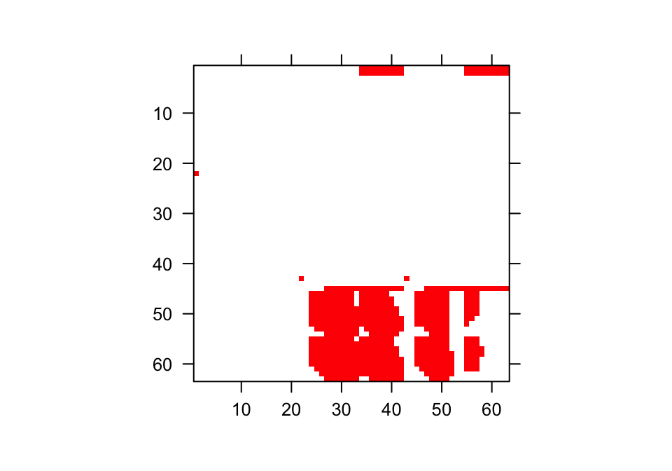
Figure 6.4: Visualization of 1st A Matrix. Red area corresponds to non-zero elements
The clear squares refer to zero elements, and the red elements refer to non-zero values corresponding to survival transitions and fecundity. The vast number of zeros may be surprising, but this matrix is a supermatrix organized by age first, with stage organizing within-age blocks. The first age is age 1, which cannot be adult, and so we find zeros in adult stages at age 1. The adult block occurs from age 2, and this block can perpetuate indefinitely. The number of elements estimated is greater now than in the typical ahistorical MPM, because now we have added age as a major factor for analysis. This matrix is overwhelmingly composed of elements that must be zero, and so it is a rather sparse matrix ((717 + 36) / 3969 = 19.0% of elements).
Given the amount of white space, we might prefer to remove impossible age-stage combinations and reduce the size of the matrices. We can do this by recreating our matrices with reduce = TRUE. Let’s try that with the main population set.
lathmat2age_red <- aflefko2(year = "all", stageframe = lathframeln,
  modelsuite = lathmodelsln2, data = lathvertln_small, supplement = lathsupp2,
  continue = TRUE, reduce = TRUE)

summary(lathmat2age_red)
>
> This ahistorical lefkoMat object contains 2 matrices.
>
> Each matrix is square with 42 rows and columns, and a total of 1764 elements.
> A total of 1434 survival transitions were estimated, with 717 per matrix.
> A total of 72 fecundity transitions were estimated, with 36 per matrix.
> This lefkoMat object covers 1 population, 1 patch, and 2 time steps.
>
> The dataset contains a total of 345 unique individuals and 531 unique transitions.
>
> Vital rate modeling quality control:
>
> Survival estimated with 247 individuals and 347 individual transitions.
> Observation estimated with 203 individuals and 294 individual transitions.
> Primary size estimated with 191 individuals and 266 individual transitions.
> Secondary size transition not estimated.
> Tertiary size transition not estimated.
> Reproductive status estimated with 191 individuals and 266 individual transitions.
> Fecundity estimated with 16 individuals and 19 individual transitions.
> Juvenile survival estimated with 184 individuals and 184 individual transitions.
> Juvenile observation estimated with 137 individuals and 137 individual transitions.
> Juvenile primary size estimated with 130 individuals and 130 individual transitions.
> Juvenile secondary size transition not estimated.
> Juvenile tertiary size transition not estimated.
> Juvenile reproduction probability not estimated.
> Juvenile maturity transition probability not estimated.
>
> Survival probability sum check (each matrix represented by column in order):
>          [,1]  [,2]
> Min.    0.000 0.000
> 1st Qu. 0.185 0.185
> Median  0.345 0.345
> Mean    0.529 0.547
> 3rd Qu. 0.995 0.996
> Max.    1.000 1.000
>
>
> Age-stages without connections leading to the rest of the life cycle found in matrices: 1 2
This exercise has eliminated 21 rows and columns, yielding a matrix with 42 rows and 42 columns. The total number of estimated elements has not changed, meaning that our matrices are much denser ((717 + 36) / 1764 = 42.7%). Let’s take a look at an image of the first matrix again (figure 6.5).
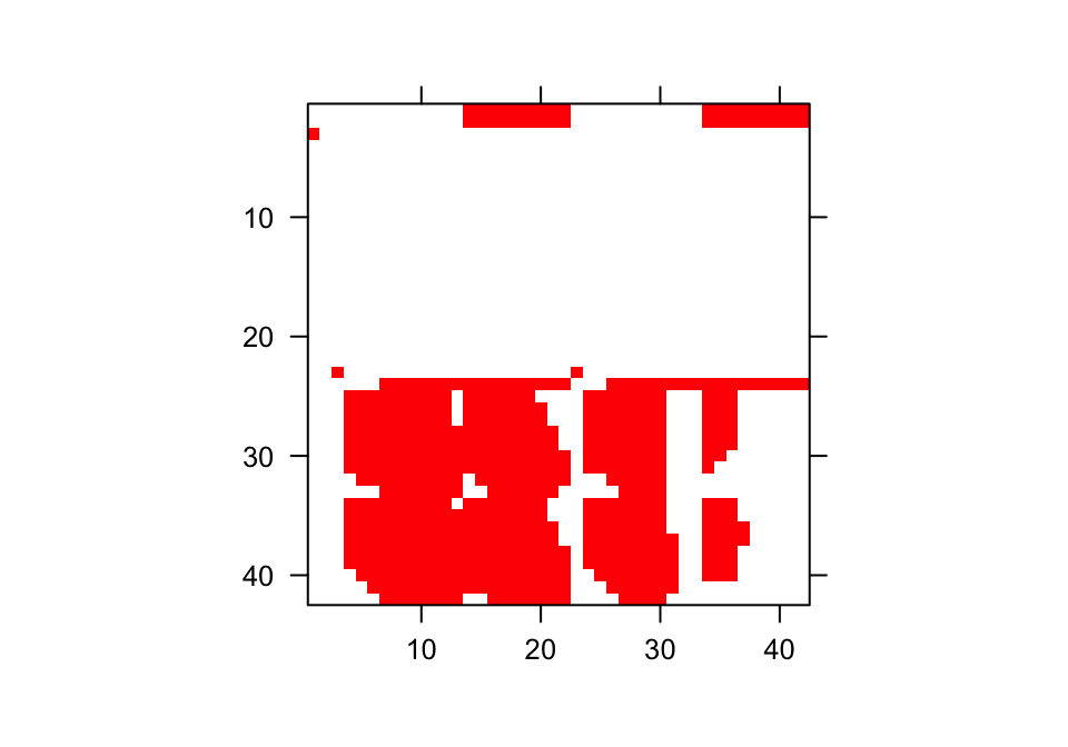
Figure 6.5: Visualization of 1st A Matrix (reduced). Red area corresponds to non-zero elements
Some of the white space has been reduced, and we see greater coverage of the matrix by non-zero elements.
We can see the order of ages and stages using the agestages element of the lefkoMat object we produced, as below. Note that our matrix is 42 rows by 42 columns, and this object gives us the exact order used.
lathmat2age_red$agestages
>    stage_id stage age
> 1         1    Sd   1
> 2         2   Sdl   1
> 3         1    Sd   2
> 4         3  Dorm   2
> 5         4 Sz1nr   2
> 6         5 Sz2nr   2
> 7         6 Sz3nr   2
> 8         7 Sz4nr   2
> 9         8 Sz5nr   2
> 10        9 Sz6nr   2
> 11       10 Sz7nr   2
> 12       11 Sz8nr   2
> 13       12 Sz9nr   2
> 14       13  Sz1r   2
> 15       14  Sz2r   2
> 16       15  Sz3r   2
> 17       16  Sz4r   2
> 18       17  Sz5r   2
> 19       18  Sz6r   2
> 20       19  Sz7r   2
> 21       20  Sz8r   2
> 22       21  Sz9r   2
> 23        1    Sd   3
> 24        3  Dorm   3
> 25        4 Sz1nr   3
> 26        5 Sz2nr   3
> 27        6 Sz3nr   3
> 28        7 Sz4nr   3
> 29        8 Sz5nr   3
> 30        9 Sz6nr   3
> 31       10 Sz7nr   3
> 32       11 Sz8nr   3
> 33       12 Sz9nr   3
> 34       13  Sz1r   3
> 35       14  Sz2r   3
> 36       15  Sz3r   3
> 37       16  Sz4r   3
> 38       17  Sz5r   3
> 39       18  Sz6r   3
> 40       19  Sz7r   3
> 41       20  Sz8r   3
> 42       21  Sz9r   3
Now let’s estimate the element-wise arithmetic mean matrices. The first lefkoMat object created will include a single mean matrix, while the second will include six mean matrices for the patches followed by a grand mean matrix, yielding a total of seven matrices.
lathmat2mean <- lmean(lathmat2age)
lathmat2pmean <- lmean(lathmat2agep)

summary(lathmat2mean)
>
> This ahistorical lefkoMat object contains 1 matrix.
>
> Each matrix is square with 63 rows and columns, and a total of 3969 elements.
> A total of 721 survival transitions were estimated, with 721 per matrix.
> A total of 36 fecundity transitions were estimated, with 36 per matrix.
> This lefkoMat object covers 1 population, 1 patch, and 0 time steps.
>
> The dataset contains a total of 345 unique individuals and 531 unique transitions.
>
> Vital rate modeling quality control:
>
> Survival estimated with 247 individuals and 347 individual transitions.
> Observation estimated with 203 individuals and 294 individual transitions.
> Primary size estimated with 191 individuals and 266 individual transitions.
> Secondary size transition not estimated.
> Tertiary size transition not estimated.
> Reproductive status estimated with 191 individuals and 266 individual transitions.
> Fecundity estimated with 16 individuals and 19 individual transitions.
> Juvenile survival estimated with 184 individuals and 184 individual transitions.
> Juvenile observation estimated with 137 individuals and 137 individual transitions.
> Juvenile primary size estimated with 130 individuals and 130 individual transitions.
> Juvenile secondary size transition not estimated.
> Juvenile tertiary size transition not estimated.
> Juvenile reproduction probability not estimated.
> Juvenile maturity transition probability not estimated.
>
> Survival probability sum check (each matrix represented by column in order):
>          [,1]
> Min.    0.000
> 1st Qu. 0.000
> Median  0.184
> Mean    0.359
> 3rd Qu. 0.912
> Max.    1.000
>
>
> Age-stages without connections leading to the rest of the life cycle found in matrices: 1
summary(lathmat2pmean)
>
> This ahistorical lefkoMat object contains 7 matrices.
>
> Each matrix is square with 63 rows and columns, and a total of 3969 elements.
> A total of 5047 survival transitions were estimated, with 721 per matrix.
> A total of 252 fecundity transitions were estimated, with 36 per matrix.
> This lefkoMat object covers 1 population, 7 patches, and 0 time steps.
>
> The dataset contains a total of 345 unique individuals and 531 unique transitions.
>
> Vital rate modeling quality control:
>
> Survival estimated with 247 individuals and 347 individual transitions.
> Observation estimated with 203 individuals and 294 individual transitions.
> Primary size estimated with 191 individuals and 266 individual transitions.
> Secondary size transition not estimated.
> Tertiary size transition not estimated.
> Reproductive status estimated with 191 individuals and 266 individual transitions.
> Fecundity estimated with 16 individuals and 19 individual transitions.
> Juvenile survival estimated with 184 individuals and 184 individual transitions.
> Juvenile observation estimated with 137 individuals and 137 individual transitions.
> Juvenile primary size estimated with 130 individuals and 130 individual transitions.
> Juvenile secondary size transition not estimated.
> Juvenile tertiary size transition not estimated.
> Juvenile reproduction probability not estimated.
> Juvenile maturity transition probability not estimated.
>
> Survival probability sum check (each matrix represented by column in order):
>          [,1]  [,2]  [,3]  [,4]  [,5]  [,6]  [,7]
> Min.    0.000 0.000 0.000 0.000 0.000 0.000 0.000
> 1st Qu. 0.000 0.000 0.000 0.000 0.000 0.000 0.000
> Median  0.881 0.823 0.874 0.757 0.816 0.861 0.843
> Mean    0.567 0.545 0.564 0.524 0.542 0.561 0.551
> 3rd Qu. 0.939 0.912 0.936 0.913 0.912 0.929 0.912
> Max.    1.000 1.000 1.000 1.000 1.000 1.000 1.000
>
>
> Age-stages without connections leading to the rest of the life cycle found in matrices: 1 2 3 4 5 6 7
We see one overall population mean in the first case, and a set of six patch-level means followed by one population mean in the second case. Note that the population mean in each case should be a little different, because the population mean in the second set weights each patch equally, while the overall population mean in the first case weights individual transitions equally regardless of patch of origin.
6.3 Developing raw age-by-stage MPMs
Now let’s focus our attention on raw (empirical) age-by-stage MPMs. For this, we will use the function arlefko2(). Raw MPMs generally require a great deal more data to parameterize properly than function-based MPMs, but we will use the same dataset as above for comparison purposes. We will also need a stageframe with fewer stages, in order to limit the number of artificial zeros entering our matrices. Let’s start with the following life history model (6.6), which assumes a total of only seven stages.
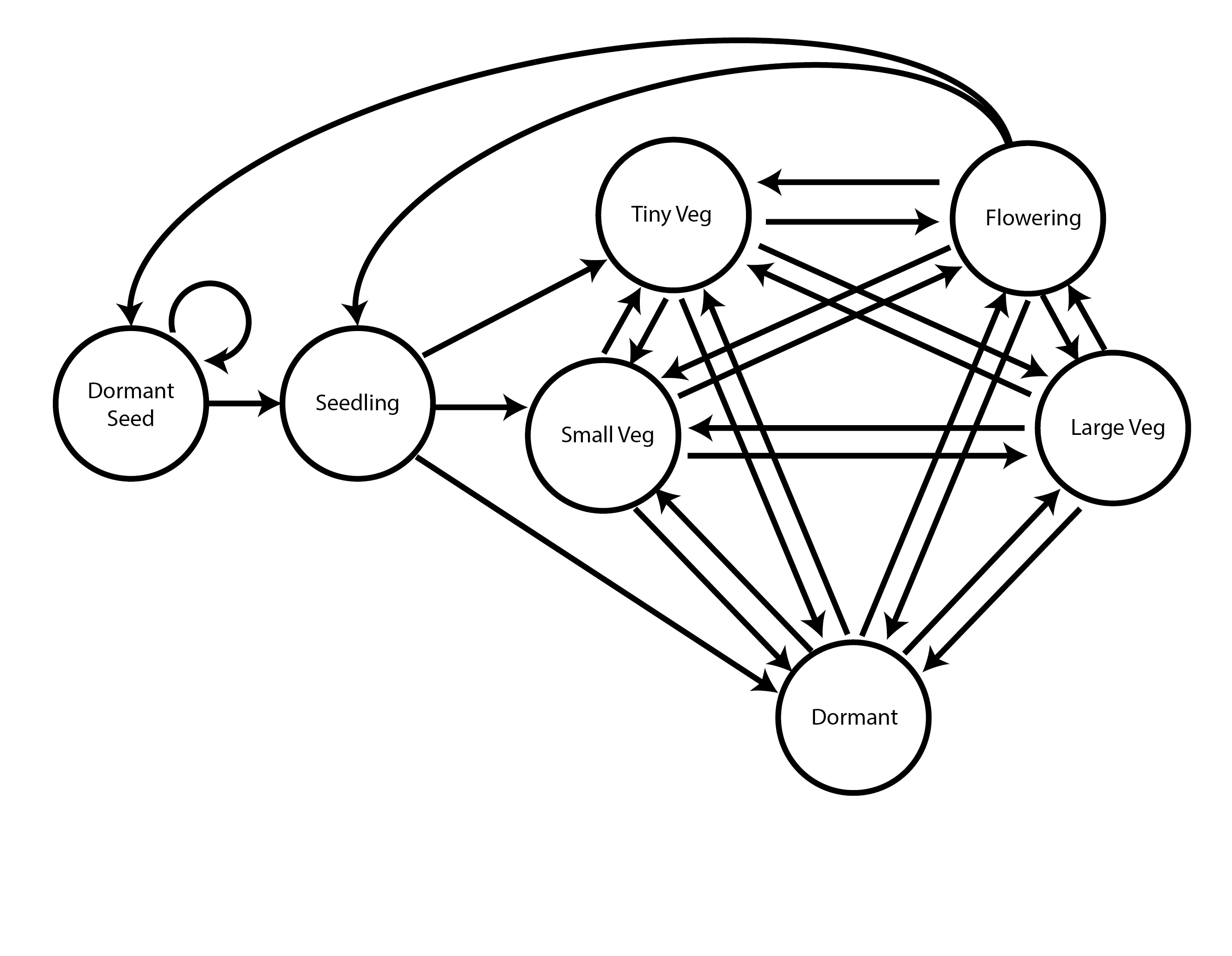
Let’s now look at our stageframe for this model. The actual stage definitions in terms of size bins are no longer based on the log leaf volume. Instead, they are based on the raw leaf volume. In order to deal with the fact that small plants are far more common than large plants, the bins have increasing widths with increasing leaf size. This will decrease the chances of missing transitions. We will also lump all reproduction into a single flowering class that can include individuals of any size, provided that they have sprouted.
sizevector <- c(0, 100, 13, 127, 3730, 3800, 0)
stagevector <- c("Sd", "Sdl", "VSm", "Sm", "VLa", "Flo", "Dorm")
repvector <- c(0, 0, 0, 0, 0, 1, 0)
obsvector <- c(0, 1, 1, 1, 1, 1, 0)
matvector <- c(0, 0, 1, 1, 1, 1, 1)
immvector <- c(1, 1, 0, 0, 0, 0, 0)
propvector <- c(1, 0, 0, 0, 0, 0, 0)
indataset <- c(0, 1, 1, 1, 1, 1, 1)
binvec <- c(0, 100, 11, 103, 3500, 3800, 0.5)

lathframe_raw <- sf_create(sizes = sizevector, stagenames = stagevector,
  repstatus = repvector, obsstatus = obsvector, matstatus = matvector,
  immstatus = immvector, indataset = indataset, binhalfwidth = binvec,
  propstatus = propvector)
lathframe_raw
>   stage size size_b size_c min_age max_age repstatus obsstatus propstatus
> 1    Sd    0     NA     NA      NA      NA         0         0          1
> 2   Sdl  100     NA     NA      NA      NA         0         1          0
> 3   VSm   13     NA     NA      NA      NA         0         1          0
> 4    Sm  127     NA     NA      NA      NA         0         1          0
> 5   VLa 3730     NA     NA      NA      NA         0         1          0
> 6   Flo 3800     NA     NA      NA      NA         1         1          0
> 7  Dorm    0     NA     NA      NA      NA         0         0          0
>   immstatus matstatus indataset binhalfwidth_raw sizebin_min sizebin_max
> 1         1         0         0              0.0         0.0         0.0
> 2         1         0         1            100.0         0.0       200.0
> 3         0         1         1             11.0         2.0        24.0
> 4         0         1         1            103.0        24.0       230.0
> 5         0         1         1           3500.0       230.0      7230.0
> 6         0         1         1           3800.0         0.0      7600.0
> 7         0         1         1              0.5        -0.5         0.5
>   sizebin_center sizebin_width binhalfwidthb_raw sizebinb_min sizebinb_max
> 1              0             0                NA           NA           NA
> 2            100           200                NA           NA           NA
> 3             13            22                NA           NA           NA
> 4            127           206                NA           NA           NA
> 5           3730          7000                NA           NA           NA
> 6           3800          7600                NA           NA           NA
> 7              0             1                NA           NA           NA
>   sizebinb_center sizebinb_width binhalfwidthc_raw sizebinc_min sizebinc_max
> 1              NA             NA                NA           NA           NA
> 2              NA             NA                NA           NA           NA
> 3              NA             NA                NA           NA           NA
> 4              NA             NA                NA           NA           NA
> 5              NA             NA                NA           NA           NA
> 6              NA             NA                NA           NA           NA
> 7              NA             NA                NA           NA           NA
>   sizebinc_center sizebinc_width group       comments
> 1              NA             NA     0 No description
> 2              NA             NA     0 No description
> 3              NA             NA     0 No description
> 4              NA             NA     0 No description
> 5              NA             NA     0 No description
> 6              NA             NA     0 No description
> 7              NA             NA     0 No description
Let’s now restandardize our core dataset, using the new stageframe for stage assignment and the original size variable for size classification. We will also cut sightings of individuals in the first year, as before, to result in a dataset in which individuals have estimated ages that we can be reasonably certain about.
lathvert_raw <- verticalize3(lathyrus, noyears = 4, firstyear = 1988,
  patchidcol = "SUBPLOT", individcol = "indiv_id", blocksize = 9,
  juvcol = "Seedling1988", sizeacol = "Volume88", repstracol = "FCODE88",
  fecacol = "Intactseed88", deadacol = "Dead1988", nonobsacol = "Dormant1988",
  stageassign = lathframe_raw, stagesize = "sizea", censorcol = "Missing1988",
  censorkeep = NA, censorRepeat = TRUE, censor = TRUE)

lathvert_raw_small <- subset(lathvert_raw, firstseen > 1988)
dim(lathvert_raw_small)
> [1] 531  54
summary_hfv(lathvert_raw_small, full = TRUE)
>
> This hfv dataset contains 531 rows, 54 variables, 1 population,
> 6 patches, 345 individuals, and 2 time steps.
>      rowid           popid              patchid        individ
>  Min.   :  30.0   Length:531         Min.   :1.000   Length:531
>  1st Qu.: 301.0   Class :character   1st Qu.:2.000   Class :character
>  Median : 582.0   Mode  :character   Median :3.000   Mode  :character
>  Mean   : 585.3                      Mean   :3.077
>  3rd Qu.: 800.5                      3rd Qu.:4.000
>  Max.   :1097.0                      Max.   :6.000
>
>      year2        firstseen       lastseen        obsage      obslifespan
>  Min.   :1989   Min.   :1989   Min.   :1989   Min.   :1.00   Min.   :0.000
>  1st Qu.:1989   1st Qu.:1989   1st Qu.:1990   1st Qu.:1.00   1st Qu.:1.000
>  Median :1990   Median :1989   Median :1991   Median :1.00   Median :2.000
>  Mean   :1990   Mean   :1989   Mean   :1991   Mean   :1.35   Mean   :1.367
>  3rd Qu.:1990   3rd Qu.:1989   3rd Qu.:1991   3rd Qu.:2.00   3rd Qu.:2.000
>  Max.   :1990   Max.   :1990   Max.   :1991   Max.   :2.00   Max.   :2.000
>
>      sizea1          size1added         repstra1        repstr1added
>  Min.   :   3.60   Min.   :   0.00   Min.   :0.00000   Min.   :0.00000
>  1st Qu.:   9.00   1st Qu.:   0.00   1st Qu.:0.00000   1st Qu.:0.00000
>  Median :  12.60   Median :   0.00   Median :0.00000   Median :0.00000
>  Mean   : 168.22   Mean   :  58.92   Mean   :0.05914   Mean   :0.02072
>  3rd Qu.:  65.22   3rd Qu.:   9.00   3rd Qu.:0.00000   3rd Qu.:0.00000
>  Max.   :4394.20   Max.   :4394.20   Max.   :1.00000   Max.   :1.00000
>  NA's   :345                         NA's   :345
>      feca1       fec1added          censor1    juvgiven1       obsstatus1
>  Min.   : 0    Min.   : 0.0000   Min.   :0   Min.   :0.000   Min.   :0.0000
>  1st Qu.: 0    1st Qu.: 0.0000   1st Qu.:0   1st Qu.:0.000   1st Qu.:0.0000
>  Median : 4    Median : 0.0000   Median :0   Median :0.000   Median :0.0000
>  Mean   : 6    Mean   : 0.1243   Mean   :0   Mean   :0.162   Mean   :0.3503
>  3rd Qu.: 6    3rd Qu.: 0.0000   3rd Qu.:0   3rd Qu.:0.000   3rd Qu.:1.0000
>  Max.   :34    Max.   :34.0000   Max.   :0   Max.   :1.000   Max.   :1.0000
>  NA's   :520
>    repstatus1        fecstatus1        matstatus1         alive1
>  Min.   :0.00000   Min.   :0.00000   Min.   :0.0000   Min.   :0.0000
>  1st Qu.:0.00000   1st Qu.:0.00000   1st Qu.:0.0000   1st Qu.:0.0000
>  Median :0.00000   Median :0.00000   Median :0.0000   Median :0.0000
>  Mean   :0.02072   Mean   :0.01318   Mean   :0.1883   Mean   :0.3503
>  3rd Qu.:0.00000   3rd Qu.:0.00000   3rd Qu.:0.0000   3rd Qu.:1.0000
>  Max.   :1.00000   Max.   :1.00000   Max.   :1.0000   Max.   :1.0000
>
>     stage1           stage1index       sizea2          size2added
>  Length:531         Min.   :0.00   Min.   :   1.80   Min.   :   0.00
>  Class :character   1st Qu.:0.00   1st Qu.:   9.00   1st Qu.:   9.00
>  Mode  :character   Median :0.00   Median :  12.60   Median :  12.60
>                     Mean   :1.09   Mean   :  99.38   Mean   :  97.88
>                     3rd Qu.:2.00   3rd Qu.:  40.80   3rd Qu.:  37.40
>                     Max.   :6.00   Max.   :4394.20   Max.   :4394.20
>                                    NA's   :8
>     repstra2        repstr2added         feca2          fec2added
>  Min.   :0.00000   Min.   :0.00000   Min.   : 0.000   Min.   : 0.000
>  1st Qu.:0.00000   1st Qu.:0.00000   1st Qu.: 0.000   1st Qu.: 0.000
>  Median :0.00000   Median :0.00000   Median : 0.000   Median : 0.000
>  Mean   :0.03633   Mean   :0.03578   Mean   : 4.053   Mean   : 0.145
>  3rd Qu.:0.00000   3rd Qu.:0.00000   3rd Qu.: 6.000   3rd Qu.: 0.000
>  Max.   :1.00000   Max.   :1.00000   Max.   :34.000   Max.   :34.000
>  NA's   :8                           NA's   :512
>     censor2    juvgiven2        obsstatus2       repstatus2
>  Min.   :0   Min.   :0.0000   Min.   :0.0000   Min.   :0.00000
>  1st Qu.:0   1st Qu.:0.0000   1st Qu.:1.0000   1st Qu.:0.00000
>  Median :0   Median :0.0000   Median :1.0000   Median :0.00000
>  Mean   :0   Mean   :0.3465   Mean   :0.9849   Mean   :0.03578
>  3rd Qu.:0   3rd Qu.:1.0000   3rd Qu.:1.0000   3rd Qu.:0.00000
>  Max.   :0   Max.   :1.0000   Max.   :1.0000   Max.   :1.00000
>
>    fecstatus2        matstatus2         alive2     stage2
>  Min.   :0.00000   Min.   :0.0000   Min.   :1   Length:531
>  1st Qu.:0.00000   1st Qu.:0.0000   1st Qu.:1   Class :character
>  Median :0.00000   Median :1.0000   Median :1   Mode  :character
>  Mean   :0.01695   Mean   :0.6535   Mean   :1
>  3rd Qu.:0.00000   3rd Qu.:1.0000   3rd Qu.:1
>  Max.   :1.00000   Max.   :1.0000   Max.   :1
>
>   stage2index        sizea3         size3added         repstra3
>  Min.   :2.000   Min.   :   2.1   Min.   :   0.00   Min.   :0.00000
>  1st Qu.:2.000   1st Qu.:  10.0   1st Qu.:   0.00   1st Qu.:0.00000
>  Median :3.000   Median :  12.6   Median :  10.50   Median :0.00000
>  Mean   :3.149   Mean   : 104.3   Mean   :  77.79   Mean   :0.05556
>  3rd Qu.:4.000   3rd Qu.:  41.1   3rd Qu.:  24.50   3rd Qu.:0.00000
>  Max.   :7.000   Max.   :6645.8   Max.   :6645.80   Max.   :1.00000
>                  NA's   :135                        NA's   :135
>   repstr3added         feca3          fec3added          censor3    juvgiven3
>  Min.   :0.00000   Min.   : 0.000   Min.   : 0.0000   Min.   :0   Min.   :0
>  1st Qu.:0.00000   1st Qu.: 0.000   1st Qu.: 0.0000   1st Qu.:0   1st Qu.:0
>  Median :0.00000   Median : 0.000   Median : 0.0000   Median :0   Median :0
>  Mean   :0.04143   Mean   : 6.045   Mean   : 0.2505   Mean   :0   Mean   :0
>  3rd Qu.:0.00000   3rd Qu.: 7.500   3rd Qu.: 0.0000   3rd Qu.:0   3rd Qu.:0
>  Max.   :1.00000   Max.   :48.000   Max.   :48.0000   Max.   :0   Max.   :0
>                    NA's   :509
>    obsstatus3       repstatus3        fecstatus3        matstatus3
>  Min.   :0.0000   Min.   :0.00000   Min.   :0.00000   Min.   :1
>  1st Qu.:0.0000   1st Qu.:0.00000   1st Qu.:0.00000   1st Qu.:1
>  Median :1.0000   Median :0.00000   Median :0.00000   Median :1
>  Mean   :0.7458   Mean   :0.04143   Mean   :0.01318   Mean   :1
>  3rd Qu.:1.0000   3rd Qu.:0.00000   3rd Qu.:0.00000   3rd Qu.:1
>  Max.   :1.0000   Max.   :1.00000   Max.   :1.00000   Max.   :1
>
>      alive3          stage3           stage3index
>  Min.   :0.0000   Length:531         Min.   :0.000
>  1st Qu.:1.0000   Class :character   1st Qu.:3.000
>  Median :1.0000   Mode  :character   Median :3.000
>  Mean   :0.8117                      Mean   :3.073
>  3rd Qu.:1.0000                      3rd Qu.:4.000
>  Max.   :1.0000                      Max.   :7.000
>
Once again we have a reduced dataset with 531 rows and 345 individuals.
Now let’s build our matrices. We will use essentially the same supplement table as before in ahistorical analysis, but we will redefine it for our new stageframe.
lathsupp2 <- supplemental(stage3 = c("Sd", "Sdl", "Sd", "Sdl"),
  stage2 = c("Sd", "Sd", "rep", "rep"), givenrate = c(0.345, 0.054, NA, NA),
  multiplier = c(NA, NA, 0.345, 0.054), type = c(1, 1, 3, 3),
  stageframe = lathframe_raw, historical = FALSE, stagebased = TRUE,
  agebased = TRUE)
> Warning: NA values in argument multiplier will be treated as 1 values.

lathmat2p_raw <- arlefko2(data = lathvert_raw_small, stageframe = lathframe_raw,
  supplement = lathsupp2, stages = c("stage3", "stage2", "stage1"),
  patch = "all", patchcol = "patchid", yearcol = "year2", agecol = "obsage",
  indivcol = "individ")

summary(lathmat2p_raw)
>
> This ahistorical lefkoMat object contains 12 matrices.
>
> Each matrix is square with 21 rows and columns, and a total of 441 elements.
> A total of 209 survival transitions were estimated, with 17.417 per matrix.
> A total of 12 fecundity transitions were estimated, with 1 per matrix.
> This lefkoMat object covers 1 population, 6 patches, and 2 time steps.
>
> The dataset contains a total of 345 unique individuals and 531 unique transitions.
>
> Survival probability sum check (each matrix represented by column in order):
>          [,1]  [,2]  [,3]  [,4]  [,5]  [,6]  [,7]  [,8]  [,9] [,10] [,11] [,12]
> Min.    0.000 0.000 0.000 0.000 0.000 0.000 0.000 0.000 0.000 0.000 0.000 0.000
> 1st Qu. 0.000 0.000 0.000 0.000 0.000 0.000 0.000 0.000 0.000 0.000 0.000 0.000
> Median  0.000 0.000 0.000 0.399 0.000 0.399 0.000 0.399 0.000 0.399 0.000 0.000
> Mean    0.281 0.349 0.261 0.385 0.274 0.463 0.268 0.423 0.223 0.388 0.234 0.279
> 3rd Qu. 0.399 0.778 0.399 0.750 0.399 1.000 0.399 0.778 0.399 0.818 0.399 0.399
> Max.    1.000 1.000 1.000 1.000 1.000 1.000 1.000 1.000 1.000 1.000 1.000 1.000
>
>
> Age-stages without connections leading to the rest of the life cycle found in matrices: 1 2 3 4 5 6 7 8 9 10 11 12
Here we have 12 matrices, each with 21 rows and columns reflecting seven stages and three ages. There are a total of 441 elements per matrix, but only an average of 18.42 are estimated per matrix due to the sparsity of data relative to the size of the matrix. Let’s take a look at the first matrix.
lathmat2p_raw$A[[1]]
>        [,1]      [,2]      [,3]   [,4]  [,5] [,6]  [,7]  [,8] [,9] [,10] [,11]
>  [1,] 0.000 0.0000000 0.0000000 0.0000 0.000    0 1.035 0.000    0     0     0
>  [2,] 0.000 0.0000000 0.0000000 0.0000 0.000    0 0.162 0.000    0     0     0
>  [3,] 0.000 0.0000000 0.0000000 0.0000 0.000    0 0.000 0.000    0     0     0
>  [4,] 0.000 0.0000000 0.0000000 0.0000 0.000    0 0.000 0.000    0     0     0
>  [5,] 0.000 0.0000000 0.0000000 0.0000 0.000    0 0.000 0.000    0     0     0
>  [6,] 0.000 0.0000000 0.0000000 0.0000 0.000    0 0.000 0.000    0     0     0
>  [7,] 0.000 0.0000000 0.0000000 0.0000 0.000    0 0.000 0.000    0     0     0
>  [8,] 0.345 0.0000000 0.0000000 0.0000 0.000    0 0.000 0.000    0     0     0
>  [9,] 0.054 0.0000000 0.0000000 0.0000 0.000    0 0.000 0.000    0     0     0
> [10,] 0.000 0.9047619 0.7142857 0.1875 0.250    0 0.000 0.000    0     0     0
> [11,] 0.000 0.0000000 0.1428571 0.6875 0.500    0 1.000 0.000    0     0     0
> [12,] 0.000 0.0000000 0.0000000 0.0000 0.000    0 0.000 0.000    0     0     0
> [13,] 0.000 0.0000000 0.0000000 0.0625 0.125    0 0.000 0.000    0     0     0
> [14,] 0.000 0.0000000 0.0000000 0.0000 0.125    0 0.000 0.000    0     0     0
> [15,] 0.000 0.0000000 0.0000000 0.0000 0.000    0 0.000 0.345    0     0     0
> [16,] 0.000 0.0000000 0.0000000 0.0000 0.000    0 0.000 0.054    0     0     0
> [17,] 0.000 0.0000000 0.0000000 0.0000 0.000    0 0.000 0.000    0     0     0
> [18,] 0.000 0.0000000 0.0000000 0.0000 0.000    0 0.000 0.000    0     0     0
> [19,] 0.000 0.0000000 0.0000000 0.0000 0.000    0 0.000 0.000    0     0     0
> [20,] 0.000 0.0000000 0.0000000 0.0000 0.000    0 0.000 0.000    0     0     0
> [21,] 0.000 0.0000000 0.0000000 0.0000 0.000    0 0.000 0.000    0     0     0
>       [,12] [,13] [,14] [,15] [,16] [,17] [,18] [,19] [,20] [,21]
>  [1,]     0     0     0 0.000     0     0     0     0     0     0
>  [2,]     0     0     0 0.000     0     0     0     0     0     0
>  [3,]     0     0     0 0.000     0     0     0     0     0     0
>  [4,]     0     0     0 0.000     0     0     0     0     0     0
>  [5,]     0     0     0 0.000     0     0     0     0     0     0
>  [6,]     0     0     0 0.000     0     0     0     0     0     0
>  [7,]     0     0     0 0.000     0     0     0     0     0     0
>  [8,]     0     0     0 0.000     0     0     0     0     0     0
>  [9,]     0     0     0 0.000     0     0     0     0     0     0
> [10,]     0     0     0 0.000     0     0     0     0     0     0
> [11,]     0     0     0 0.000     0     0     0     0     0     0
> [12,]     0     0     0 0.000     0     0     0     0     0     0
> [13,]     0     0     0 0.000     0     0     0     0     0     0
> [14,]     0     0     0 0.000     0     0     0     0     0     0
> [15,]     0     0     0 0.345     0     0     0     0     0     0
> [16,]     0     0     0 0.054     0     0     0     0     0     0
> [17,]     0     0     0 0.000     0     0     0     0     0     0
> [18,]     0     0     0 0.000     0     0     0     0     0     0
> [19,]     0     0     0 0.000     0     0     0     0     0     0
> [20,]     0     0     0 0.000     0     0     0     0     0     0
> [21,]     0     0     0 0.000     0     0     0     0     0     0
One of the more interesting problems that we can see here is the fact that since this matrix reflects a very small dataset, both in terms of numbers of observed transitions and in terms of years of observation, we cannot really estimate transitions staying within the final age. To yield such transitions, we would typically need a large and long enough dataset that we could deliberately reduce the number of ages to a number less than the longest seen, perhaps reflecting stable demographic patterns beyond some age. Clearly, here is one area in which function-based MPMs have an advantage.
To attempt to increase the number of estimated elements, let’s develop an MPM that does not differentiate patches.
lathmat2_raw <- arlefko2(data = lathvert_raw_small, stageframe = lathframe_raw,
  supplement = lathsupp2, stages = c("stage3", "stage2", "stage1"),
  yearcol = "year2", agecol = "obsage", indivcol = "individ")

summary(lathmat2_raw)
>
> This ahistorical lefkoMat object contains 2 matrices.
>
> Each matrix is square with 21 rows and columns, and a total of 441 elements.
> A total of 59 survival transitions were estimated, with 29.5 per matrix.
> A total of 6 fecundity transitions were estimated, with 3 per matrix.
> This lefkoMat object covers 1 population, 1 patch, and 2 time steps.
>
> The dataset contains a total of 345 unique individuals and 531 unique transitions.
>
> Survival probability sum check (each matrix represented by column in order):
>          [,1]  [,2]
> Min.    0.000 0.000
> 1st Qu. 0.000 0.000
> Median  0.000 0.399
> Mean    0.271 0.481
> 3rd Qu. 0.399 0.913
> Max.    1.000 1.000
>
>
> Age-stages without connections leading to the rest of the life cycle found in matrices: 1 2
Note the increase in estimated elements - now we have 32.5 elements per matrix, but only two matrices. Let’s take a look at the first matrix here.
lathmat2_raw$A[[1]]
>        [,1]       [,2]       [,3]       [,4]      [,5] [,6]       [,7]  [,8]
>  [1,] 0.000 0.00000000 0.00000000 0.00000000 0.0000000    0 2.07000000 0.000
>  [2,] 0.000 0.00000000 0.00000000 0.00000000 0.0000000    0 0.32400000 0.000
>  [3,] 0.000 0.00000000 0.00000000 0.00000000 0.0000000    0 0.00000000 0.000
>  [4,] 0.000 0.00000000 0.00000000 0.00000000 0.0000000    0 0.00000000 0.000
>  [5,] 0.000 0.00000000 0.00000000 0.00000000 0.0000000    0 0.00000000 0.000
>  [6,] 0.000 0.00000000 0.00000000 0.00000000 0.0000000    0 0.00000000 0.000
>  [7,] 0.000 0.00000000 0.00000000 0.00000000 0.0000000    0 0.00000000 0.000
>  [8,] 0.345 0.00000000 0.00000000 0.00000000 0.0000000    0 0.00000000 0.000
>  [9,] 0.054 0.00000000 0.00000000 0.00000000 0.0000000    0 0.00000000 0.000
> [10,] 0.000 0.70085470 0.78787879 0.25490196 0.1111111    0 0.00000000 0.000
> [11,] 0.000 0.02564103 0.12121212 0.52941176 0.3333333    0 0.36363636 0.000
> [12,] 0.000 0.00000000 0.00000000 0.00000000 0.2222222    0 0.27272727 0.000
> [13,] 0.000 0.02564103 0.03030303 0.05882353 0.1111111    0 0.09090909 0.000
> [14,] 0.000 0.00000000 0.00000000 0.01960784 0.1666667    0 0.27272727 0.000
> [15,] 0.000 0.00000000 0.00000000 0.00000000 0.0000000    0 0.00000000 0.345
> [16,] 0.000 0.00000000 0.00000000 0.00000000 0.0000000    0 0.00000000 0.054
> [17,] 0.000 0.00000000 0.00000000 0.00000000 0.0000000    0 0.00000000 0.000
> [18,] 0.000 0.00000000 0.00000000 0.00000000 0.0000000    0 0.00000000 0.000
> [19,] 0.000 0.00000000 0.00000000 0.00000000 0.0000000    0 0.00000000 0.000
> [20,] 0.000 0.00000000 0.00000000 0.00000000 0.0000000    0 0.00000000 0.000
> [21,] 0.000 0.00000000 0.00000000 0.00000000 0.0000000    0 0.00000000 0.000
>       [,9] [,10] [,11] [,12] [,13] [,14] [,15] [,16] [,17] [,18] [,19] [,20]
>  [1,]    0     0     0     0     0     0 0.000     0     0     0     0     0
>  [2,]    0     0     0     0     0     0 0.000     0     0     0     0     0
>  [3,]    0     0     0     0     0     0 0.000     0     0     0     0     0
>  [4,]    0     0     0     0     0     0 0.000     0     0     0     0     0
>  [5,]    0     0     0     0     0     0 0.000     0     0     0     0     0
>  [6,]    0     0     0     0     0     0 0.000     0     0     0     0     0
>  [7,]    0     0     0     0     0     0 0.000     0     0     0     0     0
>  [8,]    0     0     0     0     0     0 0.000     0     0     0     0     0
>  [9,]    0     0     0     0     0     0 0.000     0     0     0     0     0
> [10,]    0     0     0     0     0     0 0.000     0     0     0     0     0
> [11,]    0     0     0     0     0     0 0.000     0     0     0     0     0
> [12,]    0     0     0     0     0     0 0.000     0     0     0     0     0
> [13,]    0     0     0     0     0     0 0.000     0     0     0     0     0
> [14,]    0     0     0     0     0     0 0.000     0     0     0     0     0
> [15,]    0     0     0     0     0     0 0.345     0     0     0     0     0
> [16,]    0     0     0     0     0     0 0.054     0     0     0     0     0
> [17,]    0     0     0     0     0     0 0.000     0     0     0     0     0
> [18,]    0     0     0     0     0     0 0.000     0     0     0     0     0
> [19,]    0     0     0     0     0     0 0.000     0     0     0     0     0
> [20,]    0     0     0     0     0     0 0.000     0     0     0     0     0
> [21,]    0     0     0     0     0     0 0.000     0     0     0     0     0
>       [,21]
>  [1,]     0
>  [2,]     0
>  [3,]     0
>  [4,]     0
>  [5,]     0
>  [6,]     0
>  [7,]     0
>  [8,]     0
>  [9,]     0
> [10,]     0
> [11,]     0
> [12,]     0
> [13,]     0
> [14,]     0
> [15,]     0
> [16,]     0
> [17,]     0
> [18,]     0
> [19,]     0
> [20,]     0
> [21,]     0
6.4 Using supplements with age-by-stage MPMs
Supplement tables can be used to provide extra data for matrix construction according to ages as well as stages. Let’s take an example. In the previous function-based and raw MPM construction scenarios, we assumed that dormant seeds stayed dormant seeds at a rate of 0.345, and germinated at a rate of 0.054. However, suppose that we had data suggesting that two- and three-year old seed survived and germinated at only half those rates. In those cases, we would include an age vector holding the ages in time t associated with the transitions to modify, as below.
lathsupp2_age <- supplemental(stage3 =
    c("Sd", "Sdl", "Sd", "Sdl", "Sd", "Sdl", "Sd", "Sdl"),
  stage2 = c("Sd", "Sd", "Sd", "Sd", "Sd", "Sd", "rep", "rep"),
  age2 = c(1, 1, 2, 2, 3, 3, NA, NA),
  givenrate = c(0.345, 0.054, 0.173, 0.027, 0.173, 0.027, NA, NA),
  multiplier = c(NA, NA, NA, NA, NA, NA, 0.345, 0.054),
  type = c(1, 1, 1, 1, 1, 1, 3, 3), stageframe = lathframeln,
  historical = FALSE, stagebased = TRUE, agebased = TRUE)
> Warning: NA values in argument multiplier will be treated as 1 values.

lathsupp2_age
>   stage3 stage2 stage1 age2 eststage3 eststage2 eststage1 estage2 givenrate
> 1     Sd     Sd   <NA>    1      <NA>      <NA>      <NA>      NA     0.345
> 2    Sdl     Sd   <NA>    1      <NA>      <NA>      <NA>      NA     0.054
> 3     Sd     Sd   <NA>    2      <NA>      <NA>      <NA>      NA     0.173
> 4    Sdl     Sd   <NA>    2      <NA>      <NA>      <NA>      NA     0.027
> 5     Sd     Sd   <NA>    3      <NA>      <NA>      <NA>      NA     0.173
> 6    Sdl     Sd   <NA>    3      <NA>      <NA>      <NA>      NA     0.027
> 7     Sd    rep   <NA>   NA      <NA>      <NA>      <NA>      NA        NA
> 8    Sdl    rep   <NA>   NA      <NA>      <NA>      <NA>      NA        NA
>   offset multiplier convtype convtype_t12
> 1     NA      1.000        1            1
> 2     NA      1.000        1            1
> 3     NA      1.000        1            1
> 4     NA      1.000        1            1
> 5     NA      1.000        1            1
> 6     NA      1.000        1            1
> 7     NA      0.345        3            1
> 8     NA      0.054        3            1
Let’s use this new supplement to create a new raw MPM.
lathmat2p_raw_age <- arlefko2(data = lathvert_raw_small, stageframe = lathframe_raw,
  supplement = lathsupp2_age, stages = c("stage3", "stage2", "stage1"),
  patch = "all", patchcol = "patchid", yearcol = "year2", agecol = "obsage",
  indivcol = "individ")

summary(lathmat2p_raw_age)
>
> This ahistorical lefkoMat object contains 12 matrices.
>
> Each matrix is square with 21 rows and columns, and a total of 441 elements.
> A total of 209 survival transitions were estimated, with 17.417 per matrix.
> A total of 12 fecundity transitions were estimated, with 1 per matrix.
> This lefkoMat object covers 1 population, 6 patches, and 2 time steps.
>
> The dataset contains a total of 345 unique individuals and 531 unique transitions.
>
> Survival probability sum check (each matrix represented by column in order):
>          [,1]  [,2]  [,3]  [,4]  [,5]  [,6]  [,7]  [,8]  [,9] [,10] [,11] [,12]
> Min.    0.000 0.000 0.000 0.000 0.000 0.000 0.000 0.000 0.000 0.000 0.000 0.000
> 1st Qu. 0.000 0.000 0.000 0.000 0.000 0.000 0.000 0.000 0.000 0.000 0.000 0.000
> Median  0.000 0.000 0.000 0.200 0.000 0.200 0.000 0.200 0.000 0.200 0.000 0.000
> Mean    0.262 0.330 0.242 0.366 0.256 0.444 0.249 0.404 0.204 0.369 0.216 0.260
> 3rd Qu. 0.399 0.778 0.399 0.750 0.399 1.000 0.399 0.778 0.200 0.818 0.200 0.399
> Max.    1.000 1.000 1.000 1.000 1.000 1.000 1.000 1.000 1.000 1.000 1.000 1.000
>
>
> Age-stages without connections leading to the rest of the life cycle found in matrices: 1 2 3 4 5 6 7 8 9 10 11 12
The numbers of estimated elements are the same as before, because we are modifying the same elements as before. However, let’s take a look at one of the associated \(\mathbf{A}\) matrices to get an idea of what happened.
lathmat2p_raw_age$A[[1]]
>        [,1]      [,2]      [,3]   [,4]  [,5] [,6]  [,7]  [,8] [,9] [,10] [,11]
>  [1,] 0.000 0.0000000 0.0000000 0.0000 0.000    0 1.035 0.000    0     0     0
>  [2,] 0.000 0.0000000 0.0000000 0.0000 0.000    0 0.162 0.000    0     0     0
>  [3,] 0.000 0.0000000 0.0000000 0.0000 0.000    0 0.000 0.000    0     0     0
>  [4,] 0.000 0.0000000 0.0000000 0.0000 0.000    0 0.000 0.000    0     0     0
>  [5,] 0.000 0.0000000 0.0000000 0.0000 0.000    0 0.000 0.000    0     0     0
>  [6,] 0.000 0.0000000 0.0000000 0.0000 0.000    0 0.000 0.000    0     0     0
>  [7,] 0.000 0.0000000 0.0000000 0.0000 0.000    0 0.000 0.000    0     0     0
>  [8,] 0.345 0.0000000 0.0000000 0.0000 0.000    0 0.000 0.000    0     0     0
>  [9,] 0.054 0.0000000 0.0000000 0.0000 0.000    0 0.000 0.000    0     0     0
> [10,] 0.000 0.9047619 0.7142857 0.1875 0.250    0 0.000 0.000    0     0     0
> [11,] 0.000 0.0000000 0.1428571 0.6875 0.500    0 1.000 0.000    0     0     0
> [12,] 0.000 0.0000000 0.0000000 0.0000 0.000    0 0.000 0.000    0     0     0
> [13,] 0.000 0.0000000 0.0000000 0.0625 0.125    0 0.000 0.000    0     0     0
> [14,] 0.000 0.0000000 0.0000000 0.0000 0.125    0 0.000 0.000    0     0     0
> [15,] 0.000 0.0000000 0.0000000 0.0000 0.000    0 0.000 0.173    0     0     0
> [16,] 0.000 0.0000000 0.0000000 0.0000 0.000    0 0.000 0.027    0     0     0
> [17,] 0.000 0.0000000 0.0000000 0.0000 0.000    0 0.000 0.000    0     0     0
> [18,] 0.000 0.0000000 0.0000000 0.0000 0.000    0 0.000 0.000    0     0     0
> [19,] 0.000 0.0000000 0.0000000 0.0000 0.000    0 0.000 0.000    0     0     0
> [20,] 0.000 0.0000000 0.0000000 0.0000 0.000    0 0.000 0.000    0     0     0
> [21,] 0.000 0.0000000 0.0000000 0.0000 0.000    0 0.000 0.000    0     0     0
>       [,12] [,13] [,14] [,15] [,16] [,17] [,18] [,19] [,20] [,21]
>  [1,]     0     0     0 0.000     0     0     0     0     0     0
>  [2,]     0     0     0 0.000     0     0     0     0     0     0
>  [3,]     0     0     0 0.000     0     0     0     0     0     0
>  [4,]     0     0     0 0.000     0     0     0     0     0     0
>  [5,]     0     0     0 0.000     0     0     0     0     0     0
>  [6,]     0     0     0 0.000     0     0     0     0     0     0
>  [7,]     0     0     0 0.000     0     0     0     0     0     0
>  [8,]     0     0     0 0.000     0     0     0     0     0     0
>  [9,]     0     0     0 0.000     0     0     0     0     0     0
> [10,]     0     0     0 0.000     0     0     0     0     0     0
> [11,]     0     0     0 0.000     0     0     0     0     0     0
> [12,]     0     0     0 0.000     0     0     0     0     0     0
> [13,]     0     0     0 0.000     0     0     0     0     0     0
> [14,]     0     0     0 0.000     0     0     0     0     0     0
> [15,]     0     0     0 0.173     0     0     0     0     0     0
> [16,]     0     0     0 0.027     0     0     0     0     0     0
> [17,]     0     0     0 0.000     0     0     0     0     0     0
> [18,]     0     0     0 0.000     0     0     0     0     0     0
> [19,]     0     0     0 0.000     0     0     0     0     0     0
> [20,]     0     0     0 0.000     0     0     0     0     0     0
> [21,]     0     0     0 0.000     0     0     0     0     0     0
We can see the modified elements in columns 8 and 15, and these are repeated in the other \(\mathbf{A}\) and \(\mathbf{U}\) matrices. To single out the differences, let’s see the matrix difference between the MPM produced with the original supplement table, and the new MPM.
lathmat2p_raw$A[[1]] - lathmat2p_raw_age$A[[1]]
>       [,1] [,2] [,3] [,4] [,5] [,6] [,7]  [,8] [,9] [,10] [,11] [,12] [,13]
>  [1,]    0    0    0    0    0    0    0 0.000    0     0     0     0     0
>  [2,]    0    0    0    0    0    0    0 0.000    0     0     0     0     0
>  [3,]    0    0    0    0    0    0    0 0.000    0     0     0     0     0
>  [4,]    0    0    0    0    0    0    0 0.000    0     0     0     0     0
>  [5,]    0    0    0    0    0    0    0 0.000    0     0     0     0     0
>  [6,]    0    0    0    0    0    0    0 0.000    0     0     0     0     0
>  [7,]    0    0    0    0    0    0    0 0.000    0     0     0     0     0
>  [8,]    0    0    0    0    0    0    0 0.000    0     0     0     0     0
>  [9,]    0    0    0    0    0    0    0 0.000    0     0     0     0     0
> [10,]    0    0    0    0    0    0    0 0.000    0     0     0     0     0
> [11,]    0    0    0    0    0    0    0 0.000    0     0     0     0     0
> [12,]    0    0    0    0    0    0    0 0.000    0     0     0     0     0
> [13,]    0    0    0    0    0    0    0 0.000    0     0     0     0     0
> [14,]    0    0    0    0    0    0    0 0.000    0     0     0     0     0
> [15,]    0    0    0    0    0    0    0 0.172    0     0     0     0     0
> [16,]    0    0    0    0    0    0    0 0.027    0     0     0     0     0
> [17,]    0    0    0    0    0    0    0 0.000    0     0     0     0     0
> [18,]    0    0    0    0    0    0    0 0.000    0     0     0     0     0
> [19,]    0    0    0    0    0    0    0 0.000    0     0     0     0     0
> [20,]    0    0    0    0    0    0    0 0.000    0     0     0     0     0
> [21,]    0    0    0    0    0    0    0 0.000    0     0     0     0     0
>       [,14] [,15] [,16] [,17] [,18] [,19] [,20] [,21]
>  [1,]     0 0.000     0     0     0     0     0     0
>  [2,]     0 0.000     0     0     0     0     0     0
>  [3,]     0 0.000     0     0     0     0     0     0
>  [4,]     0 0.000     0     0     0     0     0     0
>  [5,]     0 0.000     0     0     0     0     0     0
>  [6,]     0 0.000     0     0     0     0     0     0
>  [7,]     0 0.000     0     0     0     0     0     0
>  [8,]     0 0.000     0     0     0     0     0     0
>  [9,]     0 0.000     0     0     0     0     0     0
> [10,]     0 0.000     0     0     0     0     0     0
> [11,]     0 0.000     0     0     0     0     0     0
> [12,]     0 0.000     0     0     0     0     0     0
> [13,]     0 0.000     0     0     0     0     0     0
> [14,]     0 0.000     0     0     0     0     0     0
> [15,]     0 0.172     0     0     0     0     0     0
> [16,]     0 0.027     0     0     0     0     0     0
> [17,]     0 0.000     0     0     0     0     0     0
> [18,]     0 0.000     0     0     0     0     0     0
> [19,]     0 0.000     0     0     0     0     0     0
> [20,]     0 0.000     0     0     0     0     0     0
> [21,]     0 0.000     0     0     0     0     0     0
We see differences only in columns 8 and 15, as expected.
Let’s now move on to Leslie MPMs.
6.5 Age-classified (Leslie) MPMs
Package lefko3 can also be used to estimate Leslie MPMs, which are purely age-based and so include no individual history. Here, we will illustrate how to create both raw and function-based Leslie MPMs using the rleslie() and fleslie() functions, respectively. We will ignore the dormant seed stage, as including dormant seeds would require using an age-by-stage approach. Our final matrices will take the following form ((6.4)).
\[\begin{equation} \left[\begin{array} {rrrr} F _{0,0} & F _{0,1} & F _{0,2} & F _{0,3} \\ S _{1,0} & 0 & 0 & 0 \\ 0 & S _{2,1} & 0 & 0 \\ 0 & 0 & S _{3,2} & S_{3,3} \\ \end{array}\right] \tag{6.4} \end{equation}\]
Normally, we would need to develop a stageframe. However, in the purely age-based case, a stageframe is unnecessary and instead all we need is the standardized hfv dataset. So, let’s start by creating that. Most of the settings will be as before. However, we need to include both NRasRep = TRUE and NOasObs = TRUE to make sure that stage classification ignores whether the individual was actually reproductive and actually observed at each time (the latter has to do with the fact that individuals can be alive with a size of zero if they are vegetatively dormant). We will also subset our data to only those individuals whose age we are reasonably sure of, by eliminating those individuals first observed in the first monitoring session.
lathvert_base <- verticalize3(lathyrus, noyears = 4, firstyear = 1988,
  patchidcol = "SUBPLOT", individcol = "indiv_id", blocksize = 9,
  sizeacol = "Volume88", repstracol = "FCODE88", fecacol = "Intactseed88",
  deadacol = "Dead1988", censorcol = "Missing1988", censorkeep = NA,
  censorRepeat= TRUE, censor = TRUE, NAas0 = TRUE, NRasRep = TRUE,
  NOasObs = TRUE)
lathvert_age <- subset(lathvert_base, firstseen > 1988)

summary_hfv(lathvert_age, full = TRUE)
>
> This hfv dataset contains 531 rows, 51 variables, 1 population,
> 6 patches, 345 individuals, and 2 time steps.
>      rowid           popid              patchid        individ
>  Min.   :  30.0   Length:531         Min.   :1.000   Length:531
>  1st Qu.: 301.0   Class :character   1st Qu.:2.000   Class :character
>  Median : 582.0   Mode  :character   Median :3.000   Mode  :character
>  Mean   : 585.3                      Mean   :3.077
>  3rd Qu.: 800.5                      3rd Qu.:4.000
>  Max.   :1097.0                      Max.   :6.000
>      year2        firstseen       lastseen        obsage      obslifespan
>  Min.   :1989   Min.   :1989   Min.   :1989   Min.   :1.00   Min.   :0.000
>  1st Qu.:1989   1st Qu.:1989   1st Qu.:1990   1st Qu.:1.00   1st Qu.:1.000
>  Median :1990   Median :1989   Median :1991   Median :1.00   Median :2.000
>  Mean   :1990   Mean   :1989   Mean   :1991   Mean   :1.35   Mean   :1.367
>  3rd Qu.:1990   3rd Qu.:1989   3rd Qu.:1991   3rd Qu.:2.00   3rd Qu.:2.000
>  Max.   :1990   Max.   :1990   Max.   :1991   Max.   :2.00   Max.   :2.000
>      sizea1          size1added         repstra1        repstr1added
>  Min.   :   0.00   Min.   :   0.00   Min.   :0.00000   Min.   :0.00000
>  1st Qu.:   0.00   1st Qu.:   0.00   1st Qu.:0.00000   1st Qu.:0.00000
>  Median :   0.00   Median :   0.00   Median :0.00000   Median :0.00000
>  Mean   :  58.92   Mean   :  58.92   Mean   :0.02072   Mean   :0.02072
>  3rd Qu.:   9.00   3rd Qu.:   9.00   3rd Qu.:0.00000   3rd Qu.:0.00000
>  Max.   :4394.20   Max.   :4394.20   Max.   :1.00000   Max.   :1.00000
>      feca1           fec1added          censor1    obsstatus1
>  Min.   : 0.0000   Min.   : 0.0000   Min.   :0   Min.   :0.0000
>  1st Qu.: 0.0000   1st Qu.: 0.0000   1st Qu.:0   1st Qu.:0.0000
>  Median : 0.0000   Median : 0.0000   Median :0   Median :0.0000
>  Mean   : 0.1243   Mean   : 0.1243   Mean   :0   Mean   :0.3503
>  3rd Qu.: 0.0000   3rd Qu.: 0.0000   3rd Qu.:0   3rd Qu.:1.0000
>  Max.   :34.0000   Max.   :34.0000   Max.   :0   Max.   :1.0000
>    repstatus1        fecstatus1        matstatus1     alive1
>  Min.   :0.00000   Min.   :0.00000   Min.   :1    Min.   :0.0000
>  1st Qu.:0.00000   1st Qu.:0.00000   1st Qu.:1    1st Qu.:0.0000
>  Median :0.00000   Median :0.00000   Median :1    Median :0.0000
>  Mean   :0.02072   Mean   :0.01318   Mean   :1    Mean   :0.3503
>  3rd Qu.:0.00000   3rd Qu.:0.00000   3rd Qu.:1    3rd Qu.:1.0000
>  Max.   :1.00000   Max.   :1.00000   Max.   :1    Max.   :1.0000
>     stage1           stage1index     sizea2          size2added
>  Length:531         Min.   :0    Min.   :   0.00   Min.   :   0.00
>  Class :character   1st Qu.:0    1st Qu.:   9.00   1st Qu.:   9.00
>  Mode  :character   Median :0    Median :  12.60   Median :  12.60
>                     Mean   :0    Mean   :  97.88   Mean   :  97.88
>                     3rd Qu.:0    3rd Qu.:  37.40   3rd Qu.:  37.40
>                     Max.   :0    Max.   :4394.20   Max.   :4394.20
>     repstra2        repstr2added         feca2          fec2added
>  Min.   :0.00000   Min.   :0.00000   Min.   : 0.000   Min.   : 0.000
>  1st Qu.:0.00000   1st Qu.:0.00000   1st Qu.: 0.000   1st Qu.: 0.000
>  Median :0.00000   Median :0.00000   Median : 0.000   Median : 0.000
>  Mean   :0.03578   Mean   :0.03578   Mean   : 0.145   Mean   : 0.145
>  3rd Qu.:0.00000   3rd Qu.:0.00000   3rd Qu.: 0.000   3rd Qu.: 0.000
>  Max.   :1.00000   Max.   :1.00000   Max.   :34.000   Max.   :34.000
>     censor2    obsstatus2       repstatus2        fecstatus2        matstatus2
>  Min.   :0   Min.   :0.0000   Min.   :0.00000   Min.   :0.00000   Min.   :1
>  1st Qu.:0   1st Qu.:1.0000   1st Qu.:0.00000   1st Qu.:0.00000   1st Qu.:1
>  Median :0   Median :1.0000   Median :0.00000   Median :0.00000   Median :1
>  Mean   :0   Mean   :0.9849   Mean   :0.03578   Mean   :0.01695   Mean   :1
>  3rd Qu.:0   3rd Qu.:1.0000   3rd Qu.:0.00000   3rd Qu.:0.00000   3rd Qu.:1
>  Max.   :0   Max.   :1.0000   Max.   :1.00000   Max.   :1.00000   Max.   :1
>      alive2     stage2           stage2index     sizea3
>  Min.   :1   Length:531         Min.   :0    Min.   :   0.00
>  1st Qu.:1   Class :character   1st Qu.:0    1st Qu.:   0.00
>  Median :1   Mode  :character   Median :0    Median :  10.50
>  Mean   :1                      Mean   :0    Mean   :  77.79
>  3rd Qu.:1                      3rd Qu.:0    3rd Qu.:  24.50
>  Max.   :1                      Max.   :0    Max.   :6645.80
>    size3added         repstra3        repstr3added         feca3
>  Min.   :   0.00   Min.   :0.00000   Min.   :0.00000   Min.   : 0.0000
>  1st Qu.:   0.00   1st Qu.:0.00000   1st Qu.:0.00000   1st Qu.: 0.0000
>  Median :  10.50   Median :0.00000   Median :0.00000   Median : 0.0000
>  Mean   :  77.79   Mean   :0.04143   Mean   :0.04143   Mean   : 0.2505
>  3rd Qu.:  24.50   3rd Qu.:0.00000   3rd Qu.:0.00000   3rd Qu.: 0.0000
>  Max.   :6645.80   Max.   :1.00000   Max.   :1.00000   Max.   :48.0000
>    fec3added          censor3    obsstatus3       repstatus3
>  Min.   : 0.0000   Min.   :0   Min.   :0.0000   Min.   :0.00000
>  1st Qu.: 0.0000   1st Qu.:0   1st Qu.:0.0000   1st Qu.:0.00000
>  Median : 0.0000   Median :0   Median :1.0000   Median :0.00000
>  Mean   : 0.2505   Mean   :0   Mean   :0.7458   Mean   :0.04143
>  3rd Qu.: 0.0000   3rd Qu.:0   3rd Qu.:1.0000   3rd Qu.:0.00000
>  Max.   :48.0000   Max.   :0   Max.   :1.0000   Max.   :1.00000
>    fecstatus3        matstatus3     alive3          stage3
>  Min.   :0.00000   Min.   :1    Min.   :0.0000   Length:531
>  1st Qu.:0.00000   1st Qu.:1    1st Qu.:1.0000   Class :character
>  Median :0.00000   Median :1    Median :1.0000   Mode  :character
>  Mean   :0.01318   Mean   :1    Mean   :0.7608
>  3rd Qu.:0.00000   3rd Qu.:1    3rd Qu.:1.0000
>  Max.   :1.00000   Max.   :1    Max.   :1.0000
>   stage3index
>  Min.   :0
>  1st Qu.:0
>  Median :0
>  Mean   :0
>  3rd Qu.:0
>  Max.   :0
So far so good! Now let’s create the vital rate models. This will go much more quickly than last time, because we no longer care about size and reproductive status as factors determining vital rates. So, we will set suite = "cons" to prevent these factors from being tested, and set age = "obsage" to incorporate our age at time t variable into all models. We will also use global.only = TRUE to prevent the age term from being dropped (normally we would not set this, but in our case the dataset is so small that age will drop out if we proceed with model selection).
lathmodels2_age <- modelsearch(lathvert_age, historical = FALSE,
  approach = "mixed", suite = "cons", bestfit = "AICc&k", age = "obsage",
  vitalrates = c("surv", "fec"), fecdist = "negbin", indiv = "individ",
  year = "year2", year.as.random = TRUE, patch.as.random = TRUE,
  show.model.tables = TRUE, fec.zero = TRUE, global.only = TRUE,
  test.age = TRUE, quiet = "partial")
Let’s see a summary of the models.
summary(lathmodels2_age)
> This LefkoMod object includes 2 linear models.
> Best-fit model criterion used: global model only
>
>
>
> Survival model:
> Generalized linear mixed model fit by maximum likelihood (Laplace
>   Approximation) [glmerMod]
>  Family: binomial  ( logit )
> Formula: alive3 ~ obsage + (1 | year2) + (1 | individ)
>    Data: surv.data
>       AIC       BIC    logLik -2*log(L)  df.resid
>  588.5991  605.6982 -290.2996  580.5991       527
> Random effects:
>  Groups  Name        Std.Dev.
>  individ (Intercept) 1.953e-05
>  year2   (Intercept) 2.988e-01
> Number of obs: 531, groups:  individ, 345; year2, 2
> Fixed Effects:
> (Intercept)       obsage
>     1.08983      0.09083
> optimizer (Nelder_Mead) convergence code: 0 (OK) ; 0 optimizer warnings; 1 lme4 warnings
>
>
>
> Observation model:
> [1] 1
>
>
>
> Size model:
> [1] 1
>
>
>
> Secondary size model:
> [1] 1
>
>
>
> Tertiary size model:
> [1] 1
>
>
>
> Reproductive status model:
> [1] 1
>
>
>
> Fecundity model:
> Formula:          feca2 ~ obsage + (1 | year2) + (1 | individ)
> Zero inflation:         ~.
> Data: fec.data
>       AIC       BIC    logLik -2*log(L)  df.resid
>        NA        NA        NA        NA       522
> Random-effects (co)variances:
>
> Conditional model:
>  Groups  Name        Std.Dev.
>  year2   (Intercept)  0.2884
>  individ (Intercept) 16.7683
>
> Zero-inflation model:
>  Groups  Name        Std.Dev.
>  year2   (Intercept) 0.9612
>  individ (Intercept) 2.6907
>
> Number of obs: 531 / Conditional model: year2, 2; individ, 345 / Zero-inflation model: year2, 2; individ, 345
>
> Dispersion parameter for nbinom2 family (): 25.3
>
> Fixed Effects:
>
> Conditional model:
> (Intercept)       obsage
>      0.7054       0.8148
>
> Zero-inflation model:
> (Intercept)       obsage
>       2.423        3.295
>
>
> Juvenile survival model:
> [1] 1
>
>
>
> Juvenile observation model:
> [1] 1
>
>
>
> Juvenile size model:
> [1] 1
>
>
>
> Juvenile secondary size model:
> [1] 1
>
>
>
> Juvenile tertiary size model:
> [1] 1
>
>
>
> Juvenile reproduction model:
> [1] 1
>
>
>
> Juvenile maturity model:
> [1] 1
>
>
>
>
>
> Number of models in survival table: 1
>
> Number of models in observation table: 1
>
> Number of models in size table: 1
>
> Number of models in secondary size table: 1
>
> Number of models in tertiary size table: 1
>
> Number of models in reproduction status table: 1
>
> Number of models in fecundity table: 1
>
> Number of models in juvenile survival table: 1
>
> Number of models in juvenile observation table: 1
>
> Number of models in juvenile size table: 1
>
> Number of models in juvenile secondary size table: 1
>
> Number of models in juvenile tertiary size table: 1
>
> Number of models in juvenile reproduction table: 1
>
> Number of models in juvenile maturity table: 1
>
>
>
>
>
> General model parameter names (column 1), and
> specific names used in these models (column 2):
>                       parameter_names mainparams
> 1                              time t      year2
> 2                          individual    individ
> 3                               patch      patch
> 4                   alive in time t+1      surv3
> 5                observed in time t+1       obs3
> 6                   sizea in time t+1      size3
> 7                   sizeb in time t+1     sizeb3
> 8                   sizec in time t+1     sizec3
> 9     reproductive status in time t+1     repst3
> 10              fecundity in time t+1       fec3
> 11                fecundity in time t       fec2
> 12                    sizea in time t      size2
> 13                  sizea in time t-1      size1
> 14                    sizeb in time t     sizeb2
> 15                  sizeb in time t-1     sizeb1
> 16                    sizec in time t     sizec2
> 17                  sizec in time t-1     sizec1
> 18      reproductive status in time t     repst2
> 19    reproductive status in time t-1     repst1
> 20        maturity status in time t+1     matst3
> 21          maturity status in time t     matst2
> 22                      age in time t        age
> 23                  density in time t    density
> 24   individual covariate a in time t   indcova2
> 25 individual covariate a in time t-1   indcova1
> 26   individual covariate b in time t   indcovb2
> 27 individual covariate b in time t-1   indcovb1
> 28   individual covariate c in time t   indcovc2
> 29 individual covariate c in time t-1   indcovc1
> 30              stage group in time t     group2
> 31            stage group in time t-1     group1
> 32       annual covariate a in time t  annucova2
> 33     annual covariate a in time t-1  annucova1
> 34       annual covariate b in time t  annucovb2
> 35     annual covariate b in time t-1  annucovb1
> 36       annual covariate c in time t  annucovc2
> 37     annual covariate c in time t-1  annucovc1
>
>
>
>
>
> Quality control:
>
> Survival model estimated with 345 individuals and 531 individual transitions.
> Survival model accuracy is 0.761.
> Observation status model not estimated.
> Primary size model not estimated.
> Secondary size model not estimated.
> Tertiary size model not estimated.
> Reproductive status model not estimated.
> Fecundity model estimated with 345 individuals and 531 individual transitions.
> Fecundity model R-squared is 0.655.
> Juvenile survival model not estimated.
> Juvenile observation status model not estimated.
> Juvenile primary size model not estimated.
> Juvenile secondary size model not estimated.
> Juvenile tertiary size model not estimated.
> Juvenile reproductive status model not estimated.
> Juvenile maturity status model not estimated.
Let’s now build a supplement table. Here, we will ignore dormant seeds and focus only on individuals from the point of germination. Thus, we no longer care about the survival rate of dormant seeds. Instead, we wish to incorporate a fecundity multiplier accounting for the germination rate. Let’s try that, as below. Note that we need to include the historical = FALSE, stagebased = FALSE, agebased = TRUE set of options for this to work properly.
lathsupp2_ageonly <- supplemental(age2 = c(2, 3), multiplier = c(0.345, 0.345),
  type = c(3, 3), historical = FALSE, stagebased = FALSE, agebased = TRUE)

lathsupp2_ageonly
>   stage3 stage2 stage1 age2 eststage3 eststage2 eststage1 estage2 givenrate
> 1   <NA>   <NA>   <NA>    2      <NA>      <NA>      <NA>      NA        NA
> 2   <NA>   <NA>   <NA>    3      <NA>      <NA>      <NA>      NA        NA
>   offset multiplier convtype convtype_t12
> 1     NA      0.345        3            1
> 2     NA      0.345        3            1
Now we will create the raw matrices. Note that this MPM does not require any set of vital rate models - only the dataset and, if appropriate, a supplement table.
lathmat2ageonly_raw <- rleslie(data = lathvert_age, year = "all",
  supplement = lathsupp2_ageonly, yearcol = "year2", indivcol = "individ")

summary(lathmat2ageonly_raw)
>
> This ahistorical lefkoMat object contains 2 matrices.
>
> Each matrix is square with 3 rows and columns, and a total of 9 elements.
> A total of 3 survival transitions were estimated, with 1.5 per matrix.
> A total of 3 fecundity transitions were estimated, with 1.5 per matrix.
> This lefkoMat object covers 1 population, 1 patch, and 2 time steps.
>
> The dataset contains a total of 345 unique individuals and 531 unique transitions.
>
> Survival probability sum check (each matrix represented by column in order):
>          [,1]  [,2]
> Min.    0.000 0.000
> 1st Qu. 0.000 0.343
> Median  0.000 0.687
> Mean    0.274 0.473
> 3rd Qu. 0.411 0.709
> Max.    0.822 0.731
>
>
> Stages without connections leading to the rest of the life cycle found in matrices: 1 2
We have just created the raw Leslie MPM. We have two matrices, because we needed to eliminate the first year of data to estimate age properly, leaving only three observation periods. The quality control looks reasonable in terms of the survival-transition probabilities falling within the range of 0.0 to 1.0. Let’s also take a look at one of the matrices, to get a handle on its structure.
lathmat2ageonly_raw$A[[2]]
>            [,1]       [,2] [,3]
> [1,] 0.02608696 0.01483871    0
> [2,] 0.68695652 0.00000000    0
> [3,] 0.00000000 0.73118280    0
Our matrix certainly looks like a valid Leslie matrix, with survival transitions in the subdiagonal and fecundity at the top. The last column is entirely composed of zeros, and that is likely due to a combination of a small dataset and a short study duration in which we cannot find individuals whom we know are older than three years old. If we view the first matrix, we will see a further column full of zeroes, as well.
Let’s now build the function-based versions and see what happens.
lathmat2ageonly_func <- fleslie(year = "all", data = lathvert_age,
  supplement = lathsupp2_ageonly, modelsuite = lathmodels2_age)

summary(lathmat2ageonly_func)
>
> This ahistorical lefkoMat object contains 2 matrices.
>
> Each matrix is square with 3 rows and columns, and a total of 9 elements.
> A total of 6 survival transitions were estimated, with 3 per matrix.
> A total of 6 fecundity transitions were estimated, with 3 per matrix.
> This lefkoMat object covers 1 population, 1 patch, and 2 time steps.
>
> The dataset contains a total of 345 unique individuals and 531 unique transitions.
>
> Vital rate modeling quality control:
>
> Survival estimated with 345 individuals and 531 individual transitions.
> Observation probability not estimated.
> Primary size transition not estimated.
> Secondary size transition not estimated.
> Tertiary size transition not estimated.
> Reproduction probability not estimated.
> Fecundity estimated with 345 individuals and 531 individual transitions.
> Juvenile survival not estimated.
> Juvenile observation probability not estimated.
> Juvenile primary size transition not estimated.
> Juvenile secondary size transition not estimated.
> Juvenile tertiary size transition not estimated.
> Juvenile reproduction probability not estimated.
> Juvenile maturity transition probability not estimated.
>
> Survival probability sum check (each matrix represented by column in order):
>          [,1]  [,2]
> Min.    0.809 0.713
> 1st Qu. 0.816 0.722
> Median  0.823 0.731
> Mean    0.822 0.731
> 3rd Qu. 0.829 0.740
> Max.    0.835 0.749
>
>
> All matrices have no stage discontinuities.
Now we have two matrices (reflecting the two estimable years). Let’s take a look at one of these matrices.
lathmat2ageonly_func$A[[2]]
>           [,1]      [,2]      [,3]
> [1,] 0.9937995 0.3449203 0.3449970
> [2,] 0.7130815 0.0000000 0.0000000
> [3,] 0.0000000 0.7312994 0.7487682
Clearly, function-based approaches have an advantage in this small, short dataset.
6.6 Age-hybrid MPMs
In some cases, we may wish to create an MPM that mostly conforms to Leslie format, but has a single stage thrown in. Such a situation may occur, for example, if we wish to build an MPM that has a dormant propagule stage, such as a plant with a dormant seed. In this case, the life of the plant from germination onward might be purely age-based, but prior to that the plant might spend an unknown number of years as a dormant seed with its own particular survival probability. Here is a sample matrix corresponding to that situation ((6.5)).
\[\begin{equation} \left[\begin{array} {rrrr} S _{1,1} & 0 & 0 & F _{1,4} \\ S _{2,1} & 0 & 0 & F _{2,4} \\ 0 & S _{3,2} & 0 & 0 \\ 0 & 0 & S _{4,3} & S _{4,4} \\ \end{array}\right] \tag{6.5} \end{equation}\]
Note that this is the same matrix as equation (6.2).
Fortunately, this is an easy situation to deal with in lefko3. First, we create a Leslie MPM without the added stage. In this case, that means repeating either the function-based or raw Leslie MPM that we already created in section 6.5. For example, here is our function-based MPM:
lathmat2ageonly_func
> $A
> $A[[1]]
>           [,1]      [,2]      [,3]
> [1,] 0.9884574 0.3448508 0.3449945
> [2,] 0.8089559 0.0000000 0.0000000
> [3,] 0.0000000 0.8226008 0.8354693
>
> $A[[2]]
>           [,1]      [,2]      [,3]
> [1,] 0.9937995 0.3449203 0.3449970
> [2,] 0.7130815 0.0000000 0.0000000
> [3,] 0.0000000 0.7312994 0.7487682
>
>
> $U
> $U[[1]]
>           [,1]      [,2]      [,3]
> [1,] 0.0000000 0.0000000 0.0000000
> [2,] 0.8089559 0.0000000 0.0000000
> [3,] 0.0000000 0.8226008 0.8354693
>
> $U[[2]]
>           [,1]      [,2]      [,3]
> [1,] 0.0000000 0.0000000 0.0000000
> [2,] 0.7130815 0.0000000 0.0000000
> [3,] 0.0000000 0.7312994 0.7487682
>
>
> $F
> $F[[1]]
>           [,1]      [,2]      [,3]
> [1,] 0.9884574 0.3448508 0.3449945
> [2,] 0.0000000 0.0000000 0.0000000
> [3,] 0.0000000 0.0000000 0.0000000
>
> $F[[2]]
>           [,1]      [,2]     [,3]
> [1,] 0.9937995 0.3449203 0.344997
> [2,] 0.0000000 0.0000000 0.000000
> [3,] 0.0000000 0.0000000 0.000000
>
>
> $ahstages
>   stage_id stage original_size original_size_b original_size_c min_age max_age
> 1        1  Age1            NA              NA              NA       1       1
> 2        2  Age2            NA              NA              NA       2       2
> 3        3  Age3            NA              NA              NA       3      NA
>   repstatus obsstatus propstatus immstatus matstatus entrystage indataset
> 1         1         1          0         0         1          1         1
> 2         1         1          0         0         1          0         1
> 3         1         1          0         0         1          0         1
>   binhalfwidth_raw sizebin_min sizebin_max sizebin_center sizebin_width
> 1               NA          NA          NA             NA            NA
> 2               NA          NA          NA             NA            NA
> 3               NA          NA          NA             NA            NA
>   binhalfwidthb_raw sizebinb_min sizebinb_max sizebinb_center sizebinb_width
> 1                NA           NA           NA              NA             NA
> 2                NA           NA           NA              NA             NA
> 3                NA           NA           NA              NA             NA
>   binhalfwidthc_raw sizebinc_min sizebinc_max sizebinc_center sizebinc_width
> 1                NA           NA           NA              NA             NA
> 2                NA           NA           NA              NA             NA
> 3                NA           NA           NA              NA             NA
>   group       comments alive almostborn
> 1     0 No description     1          0
> 2     0 No description     1          0
> 3     0 No description     1          0
>
> $agestages
>   X1
> 1 NA
>
> $hstages
>   X1
> 1 NA
>
> $labels
>   pop patch year2
> 1   1     1  1989
> 2   1     1  1990
>
> $matrixqc
> [1] 6 6 2
>
> $modelqc
>               vital_rate individuals transitions distribution  accuracy
> 1               survival         345         531     binomial 0.7608286
> 2            observation           0           0     binomial        NA
> 3                   size           0           0     gaussian        NA
> 4                  sizeb           0           0         <NA>        NA
> 5                  sizec           0           0         <NA>        NA
> 6           reproduction           0           0     binomial        NA
> 7              fecundity         345         531       negbin 0.6548547
> 8      juvenile_survival           0           0     binomial        NA
> 9    juvnile_observation           0           0     binomial        NA
> 10         juvenile_size           0           0     gaussian        NA
> 11        juvenile_sizeb           0           0         <NA>        NA
> 12        juvenile_sizec           0           0         <NA>        NA
> 13 juvenile_reproduction           0           0     binomial        NA
> 14     juvenile_maturity           0           0     binomial        NA
>
> $dataqc
> [1] 345 531
>
> attr(,"class")
> [1] "lefkoMat"
Now let’s copy this over to a new MPM with a more appropriate name for what we wish to do.
One thing to note about this MPM is that, although we did not build a stageframe for this MPM, there is nonetheless a stageframe included as this MPM’s ahstages object. Let’s take a look at that.
lathmat2_agehybrid$ahstages
>   stage_id stage original_size original_size_b original_size_c min_age max_age
> 1        1  Age1            NA              NA              NA       1       1
> 2        2  Age2            NA              NA              NA       2       2
> 3        3  Age3            NA              NA              NA       3      NA
>   repstatus obsstatus propstatus immstatus matstatus entrystage indataset
> 1         1         1          0         0         1          1         1
> 2         1         1          0         0         1          0         1
> 3         1         1          0         0         1          0         1
>   binhalfwidth_raw sizebin_min sizebin_max sizebin_center sizebin_width
> 1               NA          NA          NA             NA            NA
> 2               NA          NA          NA             NA            NA
> 3               NA          NA          NA             NA            NA
>   binhalfwidthb_raw sizebinb_min sizebinb_max sizebinb_center sizebinb_width
> 1                NA           NA           NA              NA             NA
> 2                NA           NA           NA              NA             NA
> 3                NA           NA           NA              NA             NA
>   binhalfwidthc_raw sizebinc_min sizebinc_max sizebinc_center sizebinc_width
> 1                NA           NA           NA              NA             NA
> 2                NA           NA           NA              NA             NA
> 3                NA           NA           NA              NA             NA
>   group       comments alive almostborn
> 1     0 No description     1          0
> 2     0 No description     1          0
> 3     0 No description     1          0
Next, let’s use function add_stage() to add a new stage before the first age, which is shown as Age1 in the stageframe above.
lathmat2_agehybrid <- add_stage(lathmat2_agehybrid, add_before = 1,
  stage_name = "DormSeed")

lathmat2_agehybrid
> $A
> $A[[1]]
>      [,1]      [,2]      [,3]      [,4]
> [1,]    0 0.0000000 0.0000000 0.0000000
> [2,]    0 0.9884574 0.3448508 0.3449945
> [3,]    0 0.8089559 0.0000000 0.0000000
> [4,]    0 0.0000000 0.8226008 0.8354693
>
> $A[[2]]
>      [,1]      [,2]      [,3]      [,4]
> [1,]    0 0.0000000 0.0000000 0.0000000
> [2,]    0 0.9937995 0.3449203 0.3449970
> [3,]    0 0.7130815 0.0000000 0.0000000
> [4,]    0 0.0000000 0.7312994 0.7487682
>
>
> $U
> $U[[1]]
>      [,1]      [,2]      [,3]      [,4]
> [1,]    0 0.0000000 0.0000000 0.0000000
> [2,]    0 0.0000000 0.0000000 0.0000000
> [3,]    0 0.8089559 0.0000000 0.0000000
> [4,]    0 0.0000000 0.8226008 0.8354693
>
> $U[[2]]
>      [,1]      [,2]      [,3]      [,4]
> [1,]    0 0.0000000 0.0000000 0.0000000
> [2,]    0 0.0000000 0.0000000 0.0000000
> [3,]    0 0.7130815 0.0000000 0.0000000
> [4,]    0 0.0000000 0.7312994 0.7487682
>
>
> $F
> $F[[1]]
>      [,1]      [,2]      [,3]      [,4]
> [1,]    0 0.0000000 0.0000000 0.0000000
> [2,]    0 0.9884574 0.3448508 0.3449945
> [3,]    0 0.0000000 0.0000000 0.0000000
> [4,]    0 0.0000000 0.0000000 0.0000000
>
> $F[[2]]
>      [,1]      [,2]      [,3]     [,4]
> [1,]    0 0.0000000 0.0000000 0.000000
> [2,]    0 0.9937995 0.3449203 0.344997
> [3,]    0 0.0000000 0.0000000 0.000000
> [4,]    0 0.0000000 0.0000000 0.000000
>
>
> $ahstages
>   stage_id    stage original_size original_size_b original_size_c min_age
> 1        4 DormSeed             0               0               0       0
> 2        1     Age1            NA              NA              NA       1
> 3        2     Age2            NA              NA              NA       2
> 4        3     Age3            NA              NA              NA       3
>   max_age repstatus obsstatus propstatus immstatus matstatus entrystage
> 1       0         0         1          0         1         0          1
> 2       1         1         1          0         0         1          1
> 3       2         1         1          0         0         1          0
> 4      NA         1         1          0         0         1          0
>   indataset binhalfwidth_raw sizebin_min sizebin_max sizebin_center
> 1         0                1         0.5         1.5              1
> 2         1               NA          NA          NA             NA
> 3         1               NA          NA          NA             NA
> 4         1               NA          NA          NA             NA
>   sizebin_width binhalfwidthb_raw sizebinb_min sizebinb_max sizebinb_center
> 1           0.5                 1          0.5          1.5               1
> 2            NA                NA           NA           NA              NA
> 3            NA                NA           NA           NA              NA
> 4            NA                NA           NA           NA              NA
>   sizebinb_width binhalfwidthc_raw sizebinc_min sizebinc_max sizebinc_center
> 1            0.5                 1          0.5          1.5               1
> 2             NA                NA           NA           NA              NA
> 3             NA                NA           NA           NA              NA
> 4             NA                NA           NA           NA              NA
>   sizebinc_width group       comments alive almostborn
> 1            0.5     0      new stage     1          0
> 2             NA     0 No description     1          0
> 3             NA     0 No description     1          0
> 4             NA     0 No description     1          0
>
> $agestages
>   X1
> 1 NA
>
> $hstages
>   X1
> 1 NA
>
> $labels
>   pop patch year2
> 1   1     1  1989
> 2   1     1  1990
>
> $matrixqc
> [1] 6 6 2
>
> $modelqc
>               vital_rate individuals transitions distribution  accuracy
> 1               survival         345         531     binomial 0.7608286
> 2            observation           0           0     binomial        NA
> 3                   size           0           0     gaussian        NA
> 4                  sizeb           0           0         <NA>        NA
> 5                  sizec           0           0         <NA>        NA
> 6           reproduction           0           0     binomial        NA
> 7              fecundity         345         531       negbin 0.6548547
> 8      juvenile_survival           0           0     binomial        NA
> 9    juvnile_observation           0           0     binomial        NA
> 10         juvenile_size           0           0     gaussian        NA
> 11        juvenile_sizeb           0           0         <NA>        NA
> 12        juvenile_sizec           0           0         <NA>        NA
> 13 juvenile_reproduction           0           0     binomial        NA
> 14     juvenile_maturity           0           0     binomial        NA
>
> $dataqc
> [1] 345 531
>
> attr(,"class")
> [1] "lefkoMat"
We now have a new MPM, but although the new stage that we have added is represented in the MPM, and the dimensions of the matrices have changed to 4-by-4, we still need to edit the matrix to reflect the demography of this new stage. Here, we add new survival transition probabilities and split the fecundity values between the dormant stage and the first germinated age using the edit_lM() function.
lathmat2_agehybrid$ahstages$propstatus[1] <- 1 # Dormant seeds are propagules

lathmat2_agehybrid <- edit_lM(lathmat2_agehybrid,
  stage3 = c("DormSeed", "Age1", "Age1", "DormSeed"),
  stage2 = c("DormSeed", "DormSeed", "Age3", "Age3"),
  eststage3 = c(NA, NA, NA, "Age1"),
  eststage2 = c(NA, NA, NA, "Age3"),
  givenrate = c(0.5, 0.2, NA, NA),
  multiplier = c(NA, NA, 0.5, 1),
  type = c(1, 1, 3, 2))

lathmat2_agehybrid
> $A
> $A[[1]]
>      [,1]      [,2]      [,3]      [,4]
> [1,]  0.5 0.0000000 0.0000000 0.1724972
> [2,]  0.2 0.9884574 0.3448508 0.1724972
> [3,]  0.0 0.8089559 0.0000000 0.0000000
> [4,]  0.0 0.0000000 0.8226008 0.8354693
>
> $A[[2]]
>      [,1]      [,2]      [,3]      [,4]
> [1,]  0.5 0.0000000 0.0000000 0.1724985
> [2,]  0.2 0.9937995 0.3449203 0.1724985
> [3,]  0.0 0.7130815 0.0000000 0.0000000
> [4,]  0.0 0.0000000 0.7312994 0.7487682
>
>
> $U
> $U[[1]]
>      [,1]      [,2]      [,3]      [,4]
> [1,]  0.5 0.0000000 0.0000000 0.0000000
> [2,]  0.2 0.0000000 0.0000000 0.0000000
> [3,]  0.0 0.8089559 0.0000000 0.0000000
> [4,]  0.0 0.0000000 0.8226008 0.8354693
>
> $U[[2]]
>      [,1]      [,2]      [,3]      [,4]
> [1,]  0.5 0.0000000 0.0000000 0.0000000
> [2,]  0.2 0.0000000 0.0000000 0.0000000
> [3,]  0.0 0.7130815 0.0000000 0.0000000
> [4,]  0.0 0.0000000 0.7312994 0.7487682
>
>
> $F
> $F[[1]]
>      [,1]      [,2]      [,3]      [,4]
> [1,]    0 0.0000000 0.0000000 0.1724972
> [2,]    0 0.9884574 0.3448508 0.1724972
> [3,]    0 0.0000000 0.0000000 0.0000000
> [4,]    0 0.0000000 0.0000000 0.0000000
>
> $F[[2]]
>      [,1]      [,2]      [,3]      [,4]
> [1,]    0 0.0000000 0.0000000 0.1724985
> [2,]    0 0.9937995 0.3449203 0.1724985
> [3,]    0 0.0000000 0.0000000 0.0000000
> [4,]    0 0.0000000 0.0000000 0.0000000
>
>
> $ahstages
>   stage_id    stage original_size original_size_b original_size_c min_age
> 1        4 DormSeed             0               0               0       0
> 2        1     Age1            NA              NA              NA       1
> 3        2     Age2            NA              NA              NA       2
> 4        3     Age3            NA              NA              NA       3
>   max_age repstatus obsstatus propstatus immstatus matstatus entrystage
> 1       0         0         1          1         1         0          1
> 2       1         1         1          0         0         1          1
> 3       2         1         1          0         0         1          0
> 4      NA         1         1          0         0         1          0
>   indataset binhalfwidth_raw sizebin_min sizebin_max sizebin_center
> 1         0                1         0.5         1.5              1
> 2         1               NA          NA          NA             NA
> 3         1               NA          NA          NA             NA
> 4         1               NA          NA          NA             NA
>   sizebin_width binhalfwidthb_raw sizebinb_min sizebinb_max sizebinb_center
> 1           0.5                 1          0.5          1.5               1
> 2            NA                NA           NA           NA              NA
> 3            NA                NA           NA           NA              NA
> 4            NA                NA           NA           NA              NA
>   sizebinb_width binhalfwidthc_raw sizebinc_min sizebinc_max sizebinc_center
> 1            0.5                 1          0.5          1.5               1
> 2             NA                NA           NA           NA              NA
> 3             NA                NA           NA           NA              NA
> 4             NA                NA           NA           NA              NA
>   sizebinc_width group       comments alive almostborn
> 1            0.5     0      new stage     1          0
> 2             NA     0 No description     1          0
> 3             NA     0 No description     1          0
> 4             NA     0 No description     1          0
>
> $hstages
>   X1
> 1 NA
>
> $agestages
>   X1
> 1 NA
>
> $labels
>   pop patch year2
> 1   1     1  1989
> 2   1     1  1990
>
> $dataqc
> [1] 345 531
>
> $matrixqc
> [1] 10  6  2
>
> $modelqc
>               vital_rate individuals transitions distribution  accuracy
> 1               survival         345         531     binomial 0.7608286
> 2            observation           0           0     binomial        NA
> 3                   size           0           0     gaussian        NA
> 4                  sizeb           0           0         <NA>        NA
> 5                  sizec           0           0         <NA>        NA
> 6           reproduction           0           0     binomial        NA
> 7              fecundity         345         531       negbin 0.6548547
> 8      juvenile_survival           0           0     binomial        NA
> 9    juvnile_observation           0           0     binomial        NA
> 10         juvenile_size           0           0     gaussian        NA
> 11        juvenile_sizeb           0           0         <NA>        NA
> 12        juvenile_sizec           0           0         <NA>        NA
> 13 juvenile_reproduction           0           0     binomial        NA
> 14     juvenile_maturity           0           0     binomial        NA
>
> attr(,"class")
> [1] "lefkoMat"
Everything looks quite good! Congratulations on creating your first Leslie MPMs, age-hybrid MPMs, and age-by-stage MPMs with lefko3!
6.7 Bootstrapping age-based, age-hybrid, and age-by-stage MPMs
The rules governing bootstrapping with age-based, age-hybrid, and age-by-stage MPMs are the same as those governing all other MPMs with lefko3. We initially bootstrap the hfv dataset, and use it to create the bootstrapped MPMs with the same functions we would use to make single MPMs. If we wish to create function-based MPMs, then we also need to create bootstrapped modelsuites from the bootstrapped demographic data.
Let’s start by bootstrapping raw Leslie MPMs. First, we will bootstrap the data. To make this manageable, we will only create 10 replicates.
lathvert_age_boot <- bootstrap3(lathvert_age, reps = 10)

summary_hfv(lathvert_age_boot)
>
> This hfvlist object contains 10 hfvdata demographic data frames.
> Each data frame contains an average of 526 rows, 51 variables, 1 population,
> 6 patches, 220.9 individuals, and 2 time steps.
>
> Across all data frames, there are 1 unique population, 6 unique patches, 345 unique individuals, and 2 unique time steps.
Now that we have our bootstrapped data, we just fit that into our matrix creation call.
lathmat2ageonly_raw_boot <- rleslie(data = lathvert_age_boot, year = "all",
  supplement = lathsupp2_ageonly, yearcol = "year2", indivcol = "individ")

summary(lathmat2ageonly_raw_boot)
>
> This lefkoMatList object contains 10 ahistorical lefkoMat objects.
> The average lefkoMat object contains 2 matrices.
>
> This lefkoMatList object covers an average of 1 population, 1 patch, and 2 time steps.
> Each matrix is square with 3 rows and columns, and a total of 9 elements.
> An average of 3 survival transitions were estimated in each lefkoMat object,
> with an average of 1.5 per matrix.
> An average of 2.2 fecundity transitions were estimated in each lefkoMat object,
> with an average of 1.1 per matrix.
>
> The datasets contain an average total of 215 unique individuals and 523 unique transitions.
So we have created our bootstrapped raw Leslie MPMs. What about the function-based case? For that, we will also need to create modelsuites for each of the bootstrapped data sets, as below.
set.seed(42)

lathmodels2_age_boot <- modelsearch(lathvert_age_boot, historical = FALSE,
  approach = "mixed", suite = "cons", bestfit = "AICc&k", age = "obsage",
  vitalrates = c("surv", "fec"), fecdist = "negbin", indiv = "individ",
  year = "year2", year.as.random = TRUE, patch.as.random = TRUE,
  show.model.tables = TRUE, fec.zero = TRUE, global.only = TRUE,
  test.age = TRUE, quiet = "partial")
Let’s see a summary of the bootstrapped modelsuites.
summary(lathmodels2_age_boot)
>       Length Class    Mode
>  [1,] 31     lefkoMod list
>  [2,] 31     lefkoMod list
>  [3,] 31     lefkoMod list
>  [4,] 31     lefkoMod list
>  [5,] 31     lefkoMod list
>  [6,] 31     lefkoMod list
>  [7,] 31     lefkoMod list
>  [8,] 31     lefkoMod list
>  [9,] 31     lefkoMod list
> [10,] 31     lefkoMod list
The summary output is a standard R list summary, showing us that we have 10 lefkoMod objects in object lathmodels2_age_boot. What class is this list?
Finally, let’s build the bootstrapped MPMs, and look at a summary.
lathmat2ageonly_func_boot <- fleslie(year = "all", data = lathvert_age_boot,
  supplement = lathsupp2_ageonly, modelsuite = lathmodels2_age_boot)

summary(lathmat2ageonly_func_boot)
>
> This lefkoMatList object contains 10 ahistorical lefkoMat objects.
> The average lefkoMat object contains 2 matrices.
>
> This lefkoMatList object covers an average of 1 population, 1 patch, and 2 time steps.
> Each matrix is square with 3 rows and columns, and a total of 9 elements.
> An average of 6 survival transitions were estimated in each lefkoMat object,
> with an average of 3 per matrix.
> An average of 6 fecundity transitions were estimated in each lefkoMat object,
> with an average of 3 per matrix.
>
> The datasets contain an average total of 215 unique individuals and 523 unique transitions.
>
> Vital rate modeling quality control:
>
> Survival estimated with an average of 215 individuals and 540 individual transitions.
> Observation probability not estimated.
> Primary size transition not estimated.
> Secondary size transition not estimated.
> Tertiary size transition not estimated.
> Reproduction probability not estimated.
> Fecundity estimated with an average of 215 individuals and 540 individual transitions.
> Juvenile survival not estimated.
> Juvenile observation probability not estimated.
> Juvenile primary size transition not estimated.
> Juvenile secondary size transition not estimated.
> Juvenile tertiary size transition not estimated.
> Juvenile reproduction probability not estimated.
> Juvenile maturity transition probability not estimated.
What about age-by-stage MPMs? The same procedure as before applies. Let’s start off by looking at raw Leslie MPMs. We will start by bootstrapping the data, and then creating the MPMs with the standard MPM estimation function.
lathvert_raw_small_boot <- bootstrap3(lathvert_raw_small, reps = 10)

lathmat2p_raw_boot <- arlefko2(data = lathvert_raw_small_boot, stageframe = lathframe_raw,
  supplement = lathsupp2, stages = c("stage3", "stage2", "stage1"),
  patch = "all", patchcol = "patchid", yearcol = "year2", agecol = "obsage",
  indivcol = "individ")

summary(lathmat2p_raw_boot)
>
> This lefkoMatList object contains 10 ahistorical lefkoMat objects.
> The average lefkoMat object contains 12 matrices.
>
> This lefkoMatList object covers an average of 1 population, 6 patches, and 2 time steps.
> Each matrix is square with 21 rows and columns, and a total of 441 elements.
> An average of 178.2 survival transitions were estimated in each lefkoMat object,
> with an average of 14.85 per matrix.
> An average of 9.4 fecundity transitions were estimated in each lefkoMat object,
> with an average of 0.783 per matrix.
>
> The datasets contain an average total of 216 unique individuals and 538 unique transitions.
Creating function-based MPMs is the same, but with the extra step of creating bootstrapped modelsuites.
lathvertln_small_boot <- bootstrap3(lathvertln_small, reps = 10)

lathmodelsln2_boot <- modelsearch(lathvertln_small_boot, historical = FALSE,
  approach = "mixed", suite = "full", bestfit = "AICc&k", juvestimate = "Sdl",
  vitalrates = c("surv", "obs", "size", "repst", "fec"), sizedist = "gaussian",
  fecdist = "negbin", indiv = "individ", year = "year2", age = "obsage",
  year.as.random = TRUE, patch.as.random = TRUE, show.model.tables = TRUE,
  fec.zero = TRUE, test.age = TRUE, quiet = "partial")
And now the new bootstrapped MPMs.
lathmat2age_boot <- aflefko2(year = "all", stageframe = lathframeln,
  modelsuite = lathmodelsln2_boot, data = lathvertln_small_boot,
  supplement = lathsupp2, continue = TRUE, reduce = FALSE)

summary(lathmat2age_boot)
>
> This lefkoMatList object contains 10 ahistorical lefkoMat objects.
> The average lefkoMat object contains 2 matrices.
>
> This lefkoMatList object covers an average of 1 population, 1 patch, and 2 time steps.
> Each matrix is square with 63 rows and columns, and a total of 3969 elements.
> An average of 1250.8 survival transitions were estimated in each lefkoMat object,
> with an average of 625.4 per matrix.
> An average of 72 fecundity transitions were estimated in each lefkoMat object,
> with an average of 36 per matrix.
>
> The datasets contain an average total of 225 unique individuals and 542 unique transitions.
>
> Vital rate modeling quality control:
>
> Survival estimated with an average of 159 individuals and 343 individual transitions.
> Observation estimated with an average of 129 individuals and 293 individual transitions.
> Primary size estimated with an average of 123 individuals and 264 individual transitions.
> Secondary size transition not estimated.
> Tertiary size transition not estimated.
> Reproductive status estimated with an average of 123 individuals and 264 individual transitions.
> Fecundity estimated with an average of 14 individuals and 27 individual transitions.
> Juvenile survival estimated with an average of 117 individuals and 184 individual transitions.
> Juvenile observation estimated with an average of 85 individuals and 138 individual transitions.
> Juvenile primary size estimated with an average of 84 individuals and 137 individual transitions.
> Juvenile secondary size transition not estimated.
> Juvenile tertiary size transition not estimated.
> Juvenile reproduction probability not estimated.
> Juvenile maturity transition probability not estimated.
The final case is the age-hybrid MPM. This one is a bit trickier, simply because creating this style of MPM is trickier. However, the same overall rules apply here as do for other MPMs. Let’s start off with our bootstrapped function-based Leslie MPMs. We will make a copy of it, so that we can compare it to the original
Now we will run the same functions as before on our lefkoMatList object, to add a stage and edit each component lefkoMat object with our supplemental data. However, we will also need to run a loop to change the associated propstatus vector in the stageframe for each MPM in order to show that the first stage is a propagule stage, as below.
lathmat2_agehybrid_boot <- add_stage(lathmat2_agehybrid_boot, add_before = 1,
  stage_name = "DormSeed")

for (i in c(1:10)) {
  lathmat2_agehybrid_boot[[i]]$ahstages$propstatus[1] <- 1 # Dormant seeds are propagules
}

lathmat2_agehybrid_boot <- edit_lM(lathmat2_agehybrid_boot,
  stage3 = c("DormSeed", "Age1", "Age1", "DormSeed"),
  stage2 = c("DormSeed", "DormSeed", "Age3", "Age3"),
  eststage3 = c(NA, NA, NA, "Age1"),
  eststage2 = c(NA, NA, NA, "Age3"),
  givenrate = c(0.5, 0.2, NA, NA),
  multiplier = c(NA, NA, 0.5, 1),
  type = c(1, 1, 3, 2))
Let’s take a look at just a few of these matrices to see what happened.
lathmat2_agehybrid_boot[[1]]$A[[1]]
>      [,1]      [,2]     [,3]      [,4]
> [1,]  0.5 0.0000000 0.000000 0.1725000
> [2,]  0.2 0.9999999 0.345000 0.1725000
> [3,]  0.0 1.0000000 0.000000 0.0000000
> [4,]  0.0 0.0000000 0.999998 0.1044754
lathmat2_agehybrid_boot[[2]]$A[[1]]
>      [,1]      [,2]      [,3]       [,4]
> [1,]  0.5 0.0000000 0.0000000 0.17172686
> [2,]  0.2 0.9714759 0.3410785 0.17172686
> [3,]  0.0 1.0000000 0.0000000 0.00000000
> [4,]  0.0 0.0000000 0.9999957 0.03307973
lathmat2_agehybrid_boot[[6]]$A[[1]]
>      [,1]     [,2]      [,3]       [,4]
> [1,]  0.5 0.000000 0.0000000 0.17249628
> [2,]  0.2 0.986586 0.3448132 0.17249628
> [3,]  0.0 1.000000 0.0000000 0.00000000
> [4,]  0.0 0.000000 0.9999957 0.03365221
Voilà! Now on to IPMs.
6.8 Points to remember
- Age-based (Leslie) MPMs can be be built in raw or function-based form using functions
rleslie()andfleslie(), respectively. Age-hybrid MPMs can be built using the Leslie MPM creating functions in conjunction with functionsadd_stage()andedit_lM(). Age-by-stage MPMs can be built in raw or function-based forms using functionsarlefko2()andaflefko2(), respectively.
- Age-by-stage MPMs are larger than either age-based or stage-based MPMs, and so generally require more data to parameterize properly.
- Not all possible ages need to be modeled in age-based and age-by-stage MPMs. Often, the final age in these MPMs represents a long stretch of the adult span of life during which vital rates are not expected to change dramatically, and so is capable of self-transition while other ages are not.
- Age-based MPMs are not historical and cannot be turned into historical age-based MPMs.