Chapter 14 Further Issues I: Importing Matrices and MPMs
We all reinvent our pasts.
Package lefko3 includes powerful functions to create MPMs of all major kinds. However, suppose that you already have matrices and wish to analyze them with lefko3. How can these matrices be imported properly? Our package includes functions that allow users to build lefkoMat objects with already existing matrices. Once these lefkoMat objects are built, they may be applied to the various functions found in the package for analysis.
To start, we will need to get whatever matrices we have into R itself. This may or may not be easy, depending on what format the matrices are in. Users will find it easiest to import matrices saved in standard matrix format and in lists within R object files, such as .Rda or .Rdata files. These files may be loaded into memory with the load() function. Other users may be working in R with some sort of MPM database, like COMPADRE (Salguero-Gómez et al. 2015). In other cases, users may need to import from a separate file, such as a comma-separated value (.csv) file. In this case, one approach that usually works is to use the scan() function together with matrix(), for example:
Regardless of how you accomplish this step, the goal is to take your matrix and turn it into a matrix class object in R. If a matrix or series of matrices is not too large, then perhaps the simplest way to accomplish this is to enter the matrix manually.
14.1 Creating a new lefkoMat object from imported matrices
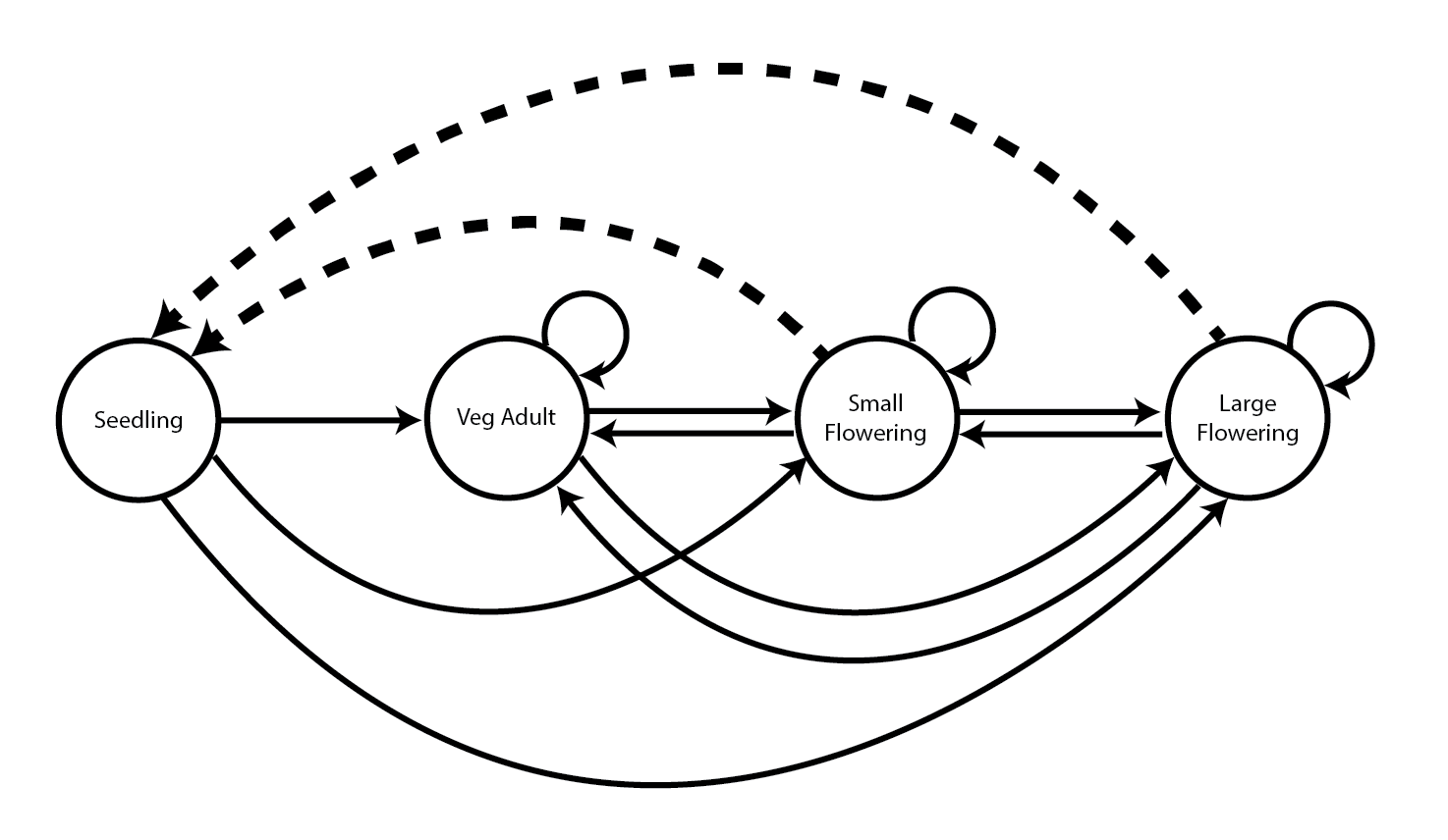
Let’s take an example using a published set of matrices. Here, we will recreate our data object anthyllis (section 1.8.3). These matrices are from Davison et al. (2010), and they report stochastic contributions made by differences in vital rate means and variances among nine natural populations of the perennial herb Anthyllis vulneraria from calcareous grasslands in Belgium. It is a short-lived, rosette-forming legume with a complex life cycle including stasis and retrogression between four stages, but no seedbank (seedlings, juveniles, small adults and large adults; figure 14.1).
Our goal in this exercise will be to import the published MPMs available for these nine populations of Anthyllis vulneraria, and to create a lefkoMat object for further study.
Of utmost importance in the process of importing matrices into lefko3 is to import the underlying life history model properly. This will require reading over whatever material describes the analyses, whether a published research paper, an unpublished thesis, or another source, and carefully listing the stages, their descriptions, and their relationships as given in survival transitions and fecundity rates. In the case of our Anthyllis analysis, this means developing the life history model in figure 14.1, and then creating a stageframe to match it.
We do not have the original demographic dataset that produced the published matrices, and so we do not really know the exact sizes used to classify stages in this analysis. However, it turns out that we do not need to know the exact sizes of plants matching the small and large adult stages, because the size data itself will not be used in any way in our own analyses. So, we will use proxy values for size in the stageframe. These proxy values need to be unique and non-negative, and they need non-overlapping bins usable as size classes defining each stage. Since we are not analyzing size itself, these proxy size values do not need any further basis in reality. Other characteristics must be exact and realistic to make sure that the analyses work properly, including reproductive status, propagule status, observation status, etc.
sizevector <- c(1, 1, 2, 3) # These sizes are not from the original paper
stagevector <- c("Sdl", "Veg", "SmFlo", "LFlo")
repvector <- c(0, 0, 1, 1)
obsvector <- c(1, 1, 1, 1)
matvector <- c(0, 1, 1, 1)
immvector <- c(1, 0, 0, 0)
propvector <- c(0, 0, 0, 0)
indataset <- c(1, 1, 1, 1)
binvec <- c(0.5, 0.5, 0.5, 0.5)
comments <- c("Seedling", "Vegetative adult", "Small flowering",
  "Large flowering")

anthframe <- sf_create(sizes = sizevector, stagenames = stagevector,
  repstatus = repvector, obsstatus = obsvector, matstatus = matvector,
  immstatus = immvector, indataset = indataset, binhalfwidth = binvec,
  propstatus = propvector, comments = comments)
anthframe
>   stage size size_b size_c min_age max_age repstatus obsstatus propstatus
> 1   Sdl    1     NA     NA      NA      NA         0         1          0
> 2   Veg    1     NA     NA      NA      NA         0         1          0
> 3 SmFlo    2     NA     NA      NA      NA         1         1          0
> 4  LFlo    3     NA     NA      NA      NA         1         1          0
>   immstatus matstatus indataset binhalfwidth_raw sizebin_min sizebin_max
> 1         1         0         1              0.5         0.5         1.5
> 2         0         1         1              0.5         0.5         1.5
> 3         0         1         1              0.5         1.5         2.5
> 4         0         1         1              0.5         2.5         3.5
>   sizebin_center sizebin_width binhalfwidthb_raw sizebinb_min sizebinb_max
> 1              1             1                NA           NA           NA
> 2              1             1                NA           NA           NA
> 3              2             1                NA           NA           NA
> 4              3             1                NA           NA           NA
>   sizebinb_center sizebinb_width binhalfwidthc_raw sizebinc_min sizebinc_max
> 1              NA             NA                NA           NA           NA
> 2              NA             NA                NA           NA           NA
> 3              NA             NA                NA           NA           NA
> 4              NA             NA                NA           NA           NA
>   sizebinc_center sizebinc_width group         comments
> 1              NA             NA     0         Seedling
> 2              NA             NA     0 Vegetative adult
> 3              NA             NA     0  Small flowering
> 4              NA             NA     0  Large flowering
Next we can enter the matrices, which were published in Davison et al. (2010). We will enter these matrices as standard matrix class objects. All matrices are square with four columns. I personally find it easier to enter matrices by row when copying from text, and so I have chosen to do so here and have indicated so in the matrix() function using byrow = TRUE (the default is to fill by column). Users familiar and comfortable with Matlab will likely be more comfortable filling matrices by row rather than by column. Here is the first matrix, covering 2003 to 2004 for population C.
XC3 <- matrix(c(0, 0, 1.74, 1.74,
  0.208333333, 0, 0, 0.057142857,
  0.041666667, 0.076923077, 0, 0,
  0.083333333, 0.076923077, 0.066666667, 0.028571429), 4, 4, byrow = TRUE)
XC3
>            [,1]       [,2]       [,3]       [,4]
> [1,] 0.00000000 0.00000000 1.74000000 1.74000000
> [2,] 0.20833333 0.00000000 0.00000000 0.05714286
> [3,] 0.04166667 0.07692308 0.00000000 0.00000000
> [4,] 0.08333333 0.07692308 0.06666667 0.02857143
This is an \(\mathbf{A}\) matrix, meaning that it includes all survival-transitions and fecundity for the population as a whole. The corresponding \(\mathbf{U}\) and \(\mathbf{F}\) matrices were not provided in that paper, although it is most likely that the elements valued at 1.74 in the top right-hand corner are only composed of fecundity values while the rest of the matrix is only composed of survival transitions (this might not be the case if clonal reproduction is possible). The order of rows and columns corresponds to the order of stages in the stageframe anthframe. Let’s now load the remaining matrices.
# POPN C 2004-2005
XC4 <- matrix(c(0, 0, 0.3, 0.6,
  0.32183908, 0.142857143, 0, 0,
  0.16091954, 0.285714286, 0, 0,
  0.252873563, 0.285714286, 0.5, 0.6), 4, 4, byrow = TRUE)

# POPN C 2005-2006
XC5 <- matrix(c(0, 0, 0.50625, 0.675,
  0, 0, 0, 0.035714286,
  0.1, 0.068965517, 0.0625, 0.107142857,
  0.3, 0.137931034, 0, 0.071428571), 4, 4, byrow = TRUE)

# POPN E 2003-2004
XE3 <- matrix(c(0, 0, 2.44, 6.569230769,
  0.196428571, 0, 0, 0,
  0.125, 0.5, 0, 0,
  0.160714286, 0.5, 0.133333333, 0.076923077), 4, 4, byrow = TRUE)

# POPN E 2004-2005
XE4 <- matrix(c(0, 0, 0.45, 0.646153846,
  0.06557377, 0.090909091, 0.125, 0,
  0.032786885, 0, 0.125, 0.076923077,
  0.049180328, 0, 0.125, 0.230769231), 4, 4, byrow = TRUE)

# POPN E 2005-2006
XE5 <- matrix(c(0, 0, 2.85, 3.99,
  0.083333333, 0, 0, 0,
  0, 0, 0, 0,
  0.416666667, 0.1, 0, 0.1), 4, 4, byrow = TRUE)

# POPN F 2003-2004
XF3 <- matrix(c(0, 0, 1.815, 7.058333333,
  0.075949367, 0, 0.05, 0.083333333,
  0.139240506, 0, 0, 0.25,
  0.075949367, 0, 0, 0.083333333), 4, 4, byrow = TRUE)

# POPN F 2004-2005
XF4 <- matrix(c(0, 0, 1.233333333, 7.4,
  0.223880597, 0, 0.111111111, 0.142857143,
  0.134328358, 0.272727273, 0.166666667, 0.142857143,
  0.119402985, 0.363636364, 0.055555556, 0.142857143), 4, 4, byrow = TRUE)

# POPN F 2005-2006
XF5 <- matrix(c(0, 0, 1.06, 3.372727273,
  0.073170732, 0.025, 0.033333333, 0,
  0.036585366, 0.15, 0.1, 0.136363636,
  0.06097561, 0.225, 0.166666667, 0.272727273), 4, 4, byrow = TRUE)

# POPN G 2003-2004
XG3 <- matrix(c(0, 0, 0.245454545, 2.1,
  0, 0, 0.045454545, 0,
  0.125, 0, 0.090909091, 0,
  0.125, 0, 0.090909091, 0.333333333), 4, 4, byrow = TRUE)

# POPN G 2004-2005
XG4 <- matrix(c(0, 0, 1.1, 1.54,
  0.111111111, 0, 0, 0,
  0, 0, 0, 0,
  0.111111111, 0, 0, 0), 4, 4, byrow = TRUE)

# POPN G 2005-2006
XG5 <- matrix(c(0, 0, 0, 1.5,
  0, 0, 0, 0,
  0.090909091, 0, 0, 0,
  0.545454545, 0.5, 0, 0.5), 4, 4, byrow = TRUE)

# POPN L 2003-2004
XL3 <- matrix(c(0, 0, 1.785365854, 1.856521739,
  0.128571429, 0, 0, 0.010869565,
  0.028571429, 0, 0, 0,
  0.014285714, 0, 0, 0.02173913), 4, 4, byrow = TRUE)

# POPN L 2004-2005
XL4 <- matrix(c(0, 0, 14.25, 16.625,
  0.131443299, 0.057142857, 0, 0.25,
  0.144329897, 0, 0, 0,
  0.092783505, 0.2, 0, 0.25), 4, 4, byrow = TRUE)

# POPN L 2005-2006
XL5 <- matrix(c(0, 0, 0.594642857, 1.765909091,
  0, 0, 0.017857143, 0,
  0.021052632, 0.018518519, 0.035714286, 0.045454545,
  0.021052632, 0.018518519, 0.035714286, 0.068181818), 4, 4, byrow = TRUE)

# POPN O 2003-2004
XO3 <- matrix(c(0, 0, 11.5, 2.775862069,
  0.6, 0.285714286, 0.333333333, 0.24137931,
  0.04, 0.142857143, 0, 0,
  0.16, 0.285714286, 0, 0.172413793), 4, 4, byrow = TRUE)

# POPN O 2004-2005
XO4 <- matrix(c(0, 0, 3.78, 1.225,
  0.28358209, 0.171052632, 0, 0.166666667,
  0.084577114, 0.026315789, 0, 0.055555556,
  0.139303483, 0.447368421, 0, 0.305555556), 4, 4, byrow = TRUE)

# POPN O 2005-2006
XO5 <- matrix(c(0, 0, 1.542857143, 1.035616438,
  0.126984127, 0.105263158, 0.047619048, 0.054794521,
  0.095238095, 0.157894737, 0.19047619, 0.082191781,
  0.111111111, 0.223684211, 0, 0.356164384), 4, 4, byrow = TRUE)

# POPN Q 2003-2004
XQ3 <- matrix(c(0, 0, 0.15, 0.175,
  0, 0, 0, 0,
  0, 0, 0, 0,
  1, 0, 0, 0), 4, 4, byrow = TRUE)

# POPN Q 2004-2005
XQ4 <- matrix(c(0, 0, 0, 0.25,
  0, 0, 0, 0,
  0, 0, 0, 0,
  1, 0.666666667, 0, 1), 4, 4, byrow = TRUE)

# POPN Q 2005-2006
XQ5 <- matrix(c(0, 0, 0, 1.428571429,
  0, 0, 0, 0.142857143,
  0.25, 0, 0, 0,
  0.25, 0, 0, 0.571428571), 4, 4, byrow = TRUE)

# POPN R 2003-2004
XR3 <- matrix(c(0, 0, 0.7, 0.6125,
  0.25, 0, 0, 0.125,
  0, 0, 0, 0,
  0.25, 0.166666667, 0, 0.25), 4, 4, byrow = TRUE)

# POPN R 2004-2005
XR4 <- matrix(c(0, 0, 0, 0.6,
  0.285714286, 0, 0, 0,
  0.285714286, 0.333333333, 0, 0,
  0.285714286, 0.333333333, 0, 1), 4, 4, byrow = TRUE)

# POPN R 2005-2006
XR5 <- matrix(c(0, 0, 0.7, 0.6125,
  0, 0, 0, 0,
  0, 0, 0, 0,
  0.333333333, 0, 0.333333333, 0.625), 4, 4, byrow = TRUE)

# POPN S 2003-2004
XS3 <- matrix(c(0, 0, 2.1, 0.816666667,
  0.166666667, 0, 0, 0,
  0, 0, 0, 0,
  0, 0, 0, 0.166666667), 4, 4, byrow = TRUE)

# POPN S 2004-2005
XS4 <- matrix(c(0, 0, 0, 7,
  0.333333333, 0.5, 0, 0,
  0, 0, 0, 0,
  0.333333333, 0, 0, 1), 4, 4, byrow = TRUE)

# POPN S 2005-2006
XS5 <- matrix(c(0, 0, 0, 1.4,
  0, 0, 0, 0,
  0, 0, 0, 0.2,
  0.111111111, 0.75, 0, 0.2), 4, 4, byrow = TRUE)
Our next step will be to incorporate these matrices into a single list of matrices. As a reminder, a list is an object in which each element can be of a different class and of different length. Let’s build our list and then inspect it.
mats_list <- list(XC3, XC4, XC5, XE3, XE4, XE5, XF3, XF4, XF5, XG3, XG4, XG5,
  XL3, XL4, XL5, XO3, XO4, XO5, XQ3, XQ4, XQ5, XR3, XR4, XR5, XS3, XS4, XS5)
mats_list
> [[1]]
>            [,1]       [,2]       [,3]       [,4]
> [1,] 0.00000000 0.00000000 1.74000000 1.74000000
> [2,] 0.20833333 0.00000000 0.00000000 0.05714286
> [3,] 0.04166667 0.07692308 0.00000000 0.00000000
> [4,] 0.08333333 0.07692308 0.06666667 0.02857143
>
> [[2]]
>           [,1]      [,2] [,3] [,4]
> [1,] 0.0000000 0.0000000  0.3  0.6
> [2,] 0.3218391 0.1428571  0.0  0.0
> [3,] 0.1609195 0.2857143  0.0  0.0
> [4,] 0.2528736 0.2857143  0.5  0.6
>
> [[3]]
>      [,1]       [,2]    [,3]       [,4]
> [1,]  0.0 0.00000000 0.50625 0.67500000
> [2,]  0.0 0.00000000 0.00000 0.03571429
> [3,]  0.1 0.06896552 0.06250 0.10714286
> [4,]  0.3 0.13793103 0.00000 0.07142857
>
> [[4]]
>           [,1] [,2]      [,3]       [,4]
> [1,] 0.0000000  0.0 2.4400000 6.56923077
> [2,] 0.1964286  0.0 0.0000000 0.00000000
> [3,] 0.1250000  0.5 0.0000000 0.00000000
> [4,] 0.1607143  0.5 0.1333333 0.07692308
>
> [[5]]
>            [,1]       [,2]  [,3]       [,4]
> [1,] 0.00000000 0.00000000 0.450 0.64615385
> [2,] 0.06557377 0.09090909 0.125 0.00000000
> [3,] 0.03278689 0.00000000 0.125 0.07692308
> [4,] 0.04918033 0.00000000 0.125 0.23076923
>
> [[6]]
>            [,1] [,2] [,3] [,4]
> [1,] 0.00000000  0.0 2.85 3.99
> [2,] 0.08333333  0.0 0.00 0.00
> [3,] 0.00000000  0.0 0.00 0.00
> [4,] 0.41666667  0.1 0.00 0.10
>
> [[7]]
>            [,1] [,2]  [,3]       [,4]
> [1,] 0.00000000    0 1.815 7.05833333
> [2,] 0.07594937    0 0.050 0.08333333
> [3,] 0.13924051    0 0.000 0.25000000
> [4,] 0.07594937    0 0.000 0.08333333
>
> [[8]]
>           [,1]      [,2]       [,3]      [,4]
> [1,] 0.0000000 0.0000000 1.23333333 7.4000000
> [2,] 0.2238806 0.0000000 0.11111111 0.1428571
> [3,] 0.1343284 0.2727273 0.16666667 0.1428571
> [4,] 0.1194030 0.3636364 0.05555556 0.1428571
>
> [[9]]
>            [,1]  [,2]       [,3]      [,4]
> [1,] 0.00000000 0.000 1.06000000 3.3727273
> [2,] 0.07317073 0.025 0.03333333 0.0000000
> [3,] 0.03658537 0.150 0.10000000 0.1363636
> [4,] 0.06097561 0.225 0.16666667 0.2727273
>
> [[10]]
>       [,1] [,2]       [,3]      [,4]
> [1,] 0.000    0 0.24545454 2.1000000
> [2,] 0.000    0 0.04545454 0.0000000
> [3,] 0.125    0 0.09090909 0.0000000
> [4,] 0.125    0 0.09090909 0.3333333
>
> [[11]]
>           [,1] [,2] [,3] [,4]
> [1,] 0.0000000    0  1.1 1.54
> [2,] 0.1111111    0  0.0 0.00
> [3,] 0.0000000    0  0.0 0.00
> [4,] 0.1111111    0  0.0 0.00
>
> [[12]]
>            [,1] [,2] [,3] [,4]
> [1,] 0.00000000  0.0    0  1.5
> [2,] 0.00000000  0.0    0  0.0
> [3,] 0.09090909  0.0    0  0.0
> [4,] 0.54545455  0.5    0  0.5
>
> [[13]]
>            [,1] [,2]     [,3]       [,4]
> [1,] 0.00000000    0 1.785366 1.85652174
> [2,] 0.12857143    0 0.000000 0.01086956
> [3,] 0.02857143    0 0.000000 0.00000000
> [4,] 0.01428571    0 0.000000 0.02173913
>
> [[14]]
>           [,1]       [,2]  [,3]   [,4]
> [1,] 0.0000000 0.00000000 14.25 16.625
> [2,] 0.1314433 0.05714286  0.00  0.250
> [3,] 0.1443299 0.00000000  0.00  0.000
> [4,] 0.0927835 0.20000000  0.00  0.250
>
> [[15]]
>            [,1]       [,2]       [,3]       [,4]
> [1,] 0.00000000 0.00000000 0.59464286 1.76590909
> [2,] 0.00000000 0.00000000 0.01785714 0.00000000
> [3,] 0.02105263 0.01851852 0.03571429 0.04545454
> [4,] 0.02105263 0.01851852 0.03571429 0.06818182
>
> [[16]]
>      [,1]      [,2]       [,3]      [,4]
> [1,] 0.00 0.0000000 11.5000000 2.7758621
> [2,] 0.60 0.2857143  0.3333333 0.2413793
> [3,] 0.04 0.1428571  0.0000000 0.0000000
> [4,] 0.16 0.2857143  0.0000000 0.1724138
>
> [[17]]
>            [,1]       [,2] [,3]       [,4]
> [1,] 0.00000000 0.00000000 3.78 1.22500000
> [2,] 0.28358209 0.17105263 0.00 0.16666667
> [3,] 0.08457711 0.02631579 0.00 0.05555556
> [4,] 0.13930348 0.44736842 0.00 0.30555556
>
> [[18]]
>           [,1]      [,2]       [,3]       [,4]
> [1,] 0.0000000 0.0000000 1.54285714 1.03561644
> [2,] 0.1269841 0.1052632 0.04761905 0.05479452
> [3,] 0.0952381 0.1578947 0.19047619 0.08219178
> [4,] 0.1111111 0.2236842 0.00000000 0.35616438
>
> [[19]]
>      [,1] [,2] [,3]  [,4]
> [1,]    0    0 0.15 0.175
> [2,]    0    0 0.00 0.000
> [3,]    0    0 0.00 0.000
> [4,]    1    0 0.00 0.000
>
> [[20]]
>      [,1]      [,2] [,3] [,4]
> [1,]    0 0.0000000    0 0.25
> [2,]    0 0.0000000    0 0.00
> [3,]    0 0.0000000    0 0.00
> [4,]    1 0.6666667    0 1.00
>
> [[21]]
>      [,1] [,2] [,3]      [,4]
> [1,] 0.00    0    0 1.4285714
> [2,] 0.00    0    0 0.1428571
> [3,] 0.25    0    0 0.0000000
> [4,] 0.25    0    0 0.5714286
>
> [[22]]
>      [,1]      [,2] [,3]   [,4]
> [1,] 0.00 0.0000000  0.7 0.6125
> [2,] 0.25 0.0000000  0.0 0.1250
> [3,] 0.00 0.0000000  0.0 0.0000
> [4,] 0.25 0.1666667  0.0 0.2500
>
> [[23]]
>           [,1]      [,2] [,3] [,4]
> [1,] 0.0000000 0.0000000    0  0.6
> [2,] 0.2857143 0.0000000    0  0.0
> [3,] 0.2857143 0.3333333    0  0.0
> [4,] 0.2857143 0.3333333    0  1.0
>
> [[24]]
>           [,1] [,2]      [,3]   [,4]
> [1,] 0.0000000    0 0.7000000 0.6125
> [2,] 0.0000000    0 0.0000000 0.0000
> [3,] 0.0000000    0 0.0000000 0.0000
> [4,] 0.3333333    0 0.3333333 0.6250
>
> [[25]]
>           [,1] [,2] [,3]      [,4]
> [1,] 0.0000000    0  2.1 0.8166667
> [2,] 0.1666667    0  0.0 0.0000000
> [3,] 0.0000000    0  0.0 0.0000000
> [4,] 0.0000000    0  0.0 0.1666667
>
> [[26]]
>           [,1] [,2] [,3] [,4]
> [1,] 0.0000000  0.0    0    7
> [2,] 0.3333333  0.5    0    0
> [3,] 0.0000000  0.0    0    0
> [4,] 0.3333333  0.0    0    1
>
> [[27]]
>           [,1] [,2] [,3] [,4]
> [1,] 0.0000000 0.00    0  1.4
> [2,] 0.0000000 0.00    0  0.0
> [3,] 0.0000000 0.00    0  0.2
> [4,] 0.1111111 0.75    0  0.2
We might now wish to check that the upper rightmost two elements are fecundity rates. One way of doing this is to duplicate this list and change the two upper rightmost elements to zero in the matrices of the duplicate list. If we are correct, then the column sums will be between 0.0 and 1.0 because the remaining transitions are all survival-transitions. R provides a number of functions to make working with lists relatively easy, and chief among these are the lapply() and unlist() functions. Let’s try this approach.
all_potential_Us <- lapply(mats_list, function(X) {
  X[1, 3] <- 0
  X[1, 4] <- 0

  return(X)
})

summary(unlist(all_potential_Us))
>    Min. 1st Qu.  Median    Mean 3rd Qu.    Max.
> 0.00000 0.00000 0.00000 0.08003 0.10000 1.00000
all_colSums <- lapply(all_potential_Us, colSums)
summary(unlist(all_colSums))
>    Min. 1st Qu.  Median    Mean 3rd Qu.    Max.
> 0.00000 0.04803 0.29557 0.32012 0.50000 1.00000
We see that we are left with values that appear to be probabilities (i.e. all range from 0.0 to 1.0), so everything looks good.
Next we will incorporate all of these matrices into a lefkoMat object. We will create the lefkoMat object to hold these matrices by calling function create_lM() with the list object we created. We will also include metadata describing the order of populations (here treated as patches), and the order of monitoring occasions.
anth_lefkoMat <- create_lM(mats = mats_list, stageframe = anthframe,
  hstages = NA, historical = FALSE, poporder = 1,
  patchorder = c("C", "C", "C", "E", "E", "E", "F", "F", "F", "G", "G", "G",
    "L", "L", "L", "O", "O", "O", "Q", "Q", "Q", "R", "R", "R", "S", "S", "S"),
  yearorder = c(2003, 2004, 2005, 2003, 2004, 2005, 2003, 2004, 2005, 2003,
    2004, 2005, 2003, 2004, 2005, 2003, 2004, 2005, 2003, 2004, 2005, 2003,
    2004, 2005, 2003, 2004, 2005))
> Warning: No supplement provided. Assuming fecundity yields all propagule and
> immature stages.
The resulting object has all of the elements of a standard lefkoMat object except for those elements related to quality control in the demographic dataset and linear modeling. The option UFdecomp was left at its default (UFdecomp = TRUE), and so create_lM() used the stageframe to infer where fecundity values were located in the matrices and created \(\mathbf{U}\) and \(\mathbf{F}\) matrices separating those values. This separation was performed on the basis of the stageframe, which shows that two stages are reproductive and that one stage acts as the entry stage for recruits into the population. The default option for historical is set to FALSE, yielding NA in place of the hstages element, which would typically list the order of historical stage pairs.
Let’s now take a look at a summary of this lefkoMat object.
summary(anth_lefkoMat)
>
> This ahistorical lefkoMat object contains 27 matrices.
>
> Each matrix is square with 4 rows and columns, and a total of 16 elements.
> A total of 167 survival transitions were estimated, with 6.185 per matrix.
> A total of 48 fecundity transitions were estimated, with 1.778 per matrix.
> This lefkoMat object covers 1 population, 9 patches, and 3 time steps.
>
> This lefkoMat object appears to have been imported. Number of unique individuals and transitions not known.
>
> Survival probability sum check (each matrix represented by column in order):
>           [,1]  [,2]   [,3]   [,4]   [,5]  [,6]   [,7]  [,8]  [,9] [,10]  [,11]
> Min.    0.0667 0.500 0.0625 0.0769 0.0909 0.000 0.0000 0.333 0.171 0.000 0.0000
> 1st Qu. 0.0810 0.575 0.1708 0.1192 0.1334 0.075 0.0375 0.405 0.268 0.170 0.0000
> Median  0.1198 0.657 0.2106 0.3077 0.2276 0.100 0.1706 0.453 0.350 0.239 0.0000
> Mean    0.1599 0.637 0.2209 0.4231 0.2303 0.175 0.1895 0.469 0.320 0.203 0.0556
> 3rd Qu. 0.1987 0.720 0.2607 0.6116 0.3245 0.200 0.3225 0.517 0.402 0.271 0.0556
> Max.    0.3333 0.736 0.4000 1.0000 0.3750 0.500 0.4167 0.636 0.409 0.333 0.2222
>         [,12]  [,13] [,14]  [,15] [,16] [,17] [,18] [,19] [,20] [,21] [,22]
> Min.    0.000 0.0000 0.000 0.0370 0.333 0.000 0.238  0.00 0.000 0.000 0.000
> 1st Qu. 0.375 0.0000 0.193 0.0408 0.394 0.381 0.310  0.00 0.500 0.000 0.125
> Median  0.500 0.0163 0.313 0.0657 0.564 0.518 0.410  0.00 0.833 0.250 0.271
> Mean    0.409 0.0510 0.281 0.0705 0.565 0.420 0.388  0.25 0.667 0.304 0.260
> 3rd Qu. 0.534 0.0673 0.401 0.0954 0.736 0.557 0.488  0.25 1.000 0.554 0.406
> Max.    0.636 0.1714 0.500 0.1136 0.800 0.645 0.493  1.00 1.000 0.714 0.500
>         [,23] [,24]  [,25] [,26]  [,27]
> Min.    0.000 0.000 0.0000 0.000 0.0000
> 1st Qu. 0.500 0.250 0.0000 0.375 0.0833
> Median  0.762 0.333 0.0833 0.583 0.2556
> Mean    0.631 0.323 0.0833 0.542 0.3153
> 3rd Qu. 0.893 0.406 0.1667 0.750 0.4875
> Max.    1.000 0.625 0.1667 1.000 0.7500
>
>
> Stages without connections leading to the rest of the life cycle found in matrices: 5 7 10 11 12 13 19 20 21 23 24 25 26 27
The summary of this new lefkoMat object shows us that we have 27 matrices with four rows and columns each. The estimated numbers of transitions corresponds to the non-zero entries in each matrix. We see that we are covering one population, nine patches, and three time steps. All of the survival probabilities observed fall within the bounds of 0.0 to 1.0, so everything seems alright. A number of matrices have dead-end stages, but that is likely because the matrices are empirical. At this point, we can use this object in lefko3’s various projection analyses.
14.2 Importing matrices from COMPADRE and COMADRE
Users may be aware of the amazing MPM databases COMPADRE and COMADRE, which were created and are maintained with the aim of holding all published MPMs in open, online repositories (Salguero-Gómez et al. 2015, 2016). The former covers MPMs for plants, fungi, and microbes, while the latter covers animals. The create_lM() function, which is the means to important lists of matrices, also allows matrices to be imported into lefkoMat format from these databases. We encourage users to explore package Rcompadre, which includes a host of functions to allow the exploration of these databases (Jones et al. 2022). We will also make use of one function from this package in our code below, although this is not required.
To start, we need to access one of these databases for use. There are two approaches that we might use. First, we can download the database of interest from the web - they are available at https://compadre-db.org/. Alternatively, we can download a database using the cdb_fetch() function in Rcompadre. In the next block, we load both databases after downloading them manually (the user will need to download them on their own initiative to use the code below, and will also need to update the code with the newest database file names).
load("COMPADRE_v.6.25.8.0.RData")
load("COMADRE_v.4.25.8.1.RData")

summary(compadre)
>             Length Class      Mode
> metadata      58   data.frame list
> matrixClass 9146   -none-     list
> mat         9146   -none-     list
> version        7   -none-     list
summary(comadre)
>             Length Class      Mode
> metadata      58   data.frame list
> matrixClass 3550   -none-     list
> mat         3550   -none-     list
> version        7   -none-     list
In the next block, we use Rcompadre to download the databases (note that the following code may fail depending on the current status of the online databases).
Users will notice discrepancies in the summaries of the databases downloaded manually from the web vs those downloaded using Rcompadre. The database structure differs somewhat, but the data is essentially the same, and lefko3 can handle both structures.
Once the databases are in R’s global environment, users can search them for MPMs of interest. The databases may be searched to find published papers, species or other taxa, locations, and other characteristics of interest. Regardless of what characteristics the user is looking for, it is important to remember that lefko3 can only produce lefkoMat objects with matrices of the same dimension, because a single lefkoMat object is meant to hold a single MPM. Therefore, matrices of different dimensions will lead to fatal errors in processing.
In the code below, we create a new lefkoMat object using four separate matrices. These matrices cover a population of the seaweed Ascophyllum nodosum, surveyed near the city of Göteberg, Sweden (Åberg 1990).
mpm_a <- create_lM(matrix_id = c(238271, 238272, 238273, 238274), mats = compadre)
summary(mpm_a)
>
> This ahistorical lefkoMat object contains 4 matrices.
>
> Each matrix is square with 5 rows and columns, and a total of 25 elements.
> A total of 63 survival transitions were estimated, with 15.75 per matrix.
> A total of 16 fecundity transitions were estimated, with 4 per matrix.
> This lefkoMat object covers 1 population, 1 patch, and 1 time step.
>
> This lefkoMat object appears to have been imported. Number of unique individuals and transitions not known.
>
> Survival probability sum check (each matrix represented by column in order):
>          [,1]  [,2] [,3]  [,4]
> Min.    0.630 0.800 0.28 0.240
> 1st Qu. 0.630 0.830 0.45 0.290
> Median  0.770 0.960 0.50 0.310
> Mean    0.754 0.918 0.51 0.362
> 3rd Qu. 0.820 1.000 0.52 0.370
> Max.    0.920 1.000 0.80 0.600
>
>
> All matrices have no stage discontinuities.
Note that the summary looks exactly as a lefkoMat object summary should. Let’s dig into the MPM structure a bit, as well.
mpm_a
> $A
> $A[[1]]
>        A1   A2   A3   A4   A5
> [1,] 0.48 0.30 0.70 2.39 7.84
> [2,] 0.13 0.28 0.07 0.03 0.01
> [3,] 0.02 0.33 0.40 0.19 0.04
> [4,] 0.00 0.02 0.29 0.41 0.57
> [5,] 0.00 0.00 0.01 0.19 0.30
>
> $A[[2]]
>        A1   A2   A3   A4   A5
> [1,] 0.55 0.32 0.64 2.37 7.82
> [2,] 0.25 0.33 0.06 0.00 0.00
> [3,] 0.03 0.45 0.50 0.18 0.00
> [4,] 0.00 0.02 0.40 0.55 0.60
> [5,] 0.00 0.00 0.00 0.27 0.40
>
> $A[[3]]
>        A1   A2   A3   A4   A5
> [1,] 0.38 0.23 0.79 2.40 7.82
> [2,] 0.11 0.18 0.10 0.07 0.00
> [3,] 0.01 0.10 0.23 0.26 0.10
> [4,] 0.00 0.00 0.10 0.15 0.60
> [5,] 0.00 0.00 0.02 0.04 0.10
>
> $A[[4]]
>        A1   A2   A3   A4   A5
> [1,] 0.28 0.46 0.85 2.58 8.05
> [2,] 0.02 0.15 0.09 0.11 0.15
> [3,] 0.01 0.09 0.20 0.04 0.15
> [4,] 0.00 0.00 0.00 0.18 0.15
> [5,] 0.00 0.00 0.00 0.04 0.15
>
>
> $U
> $U[[1]]
>        U1   U2   U3   U4   U5
> [1,] 0.48 0.00 0.00 0.00 0.00
> [2,] 0.13 0.28 0.07 0.03 0.01
> [3,] 0.02 0.33 0.40 0.19 0.04
> [4,] 0.00 0.02 0.29 0.41 0.57
> [5,] 0.00 0.00 0.01 0.19 0.30
>
> $U[[2]]
>        U1   U2   U3   U4  U5
> [1,] 0.55 0.00 0.00 0.00 0.0
> [2,] 0.25 0.33 0.06 0.00 0.0
> [3,] 0.03 0.45 0.50 0.18 0.0
> [4,] 0.00 0.02 0.40 0.55 0.6
> [5,] 0.00 0.00 0.00 0.27 0.4
>
> $U[[3]]
>        U1   U2   U3   U4  U5
> [1,] 0.38 0.00 0.00 0.00 0.0
> [2,] 0.11 0.18 0.10 0.07 0.0
> [3,] 0.01 0.10 0.23 0.26 0.1
> [4,] 0.00 0.00 0.10 0.15 0.6
> [5,] 0.00 0.00 0.02 0.04 0.1
>
> $U[[4]]
>        U1   U2   U3   U4   U5
> [1,] 0.28 0.00 0.00 0.00 0.00
> [2,] 0.02 0.15 0.09 0.11 0.15
> [3,] 0.01 0.09 0.20 0.04 0.15
> [4,] 0.00 0.00 0.00 0.18 0.15
> [5,] 0.00 0.00 0.00 0.04 0.15
>
>
> $F
> $F[[1]]
>      F1  F2  F3   F4   F5
> [1,]  0 0.3 0.7 2.39 7.84
> [2,]  0 0.0 0.0 0.00 0.00
> [3,]  0 0.0 0.0 0.00 0.00
> [4,]  0 0.0 0.0 0.00 0.00
> [5,]  0 0.0 0.0 0.00 0.00
>
> $F[[2]]
>      F1   F2   F3   F4   F5
> [1,]  0 0.32 0.64 2.37 7.82
> [2,]  0 0.00 0.00 0.00 0.00
> [3,]  0 0.00 0.00 0.00 0.00
> [4,]  0 0.00 0.00 0.00 0.00
> [5,]  0 0.00 0.00 0.00 0.00
>
> $F[[3]]
>      F1   F2   F3  F4   F5
> [1,]  0 0.23 0.79 2.4 7.82
> [2,]  0 0.00 0.00 0.0 0.00
> [3,]  0 0.00 0.00 0.0 0.00
> [4,]  0 0.00 0.00 0.0 0.00
> [5,]  0 0.00 0.00 0.0 0.00
>
> $F[[4]]
>      F1   F2   F3   F4   F5
> [1,]  0 0.46 0.85 2.58 8.05
> [2,]  0 0.00 0.00 0.00 0.00
> [3,]  0 0.00 0.00 0.00 0.00
> [4,]  0 0.00 0.00 0.00 0.00
> [5,]  0 0.00 0.00 0.00 0.00
>
>
> $ahstages
>   stage_id   stage size size_b size_c min_age max_age repstatus obsstatus
> 1        1 stage 1    1      0      0       0       0         0         1
> 2        2 stage 2    2      0      0       0       0         1         1
> 3        3 stage 3    3      0      0       0       0         1         1
> 4        4 stage 4    4      0      0       0       0         1         1
> 5        5 stage 5    5      0      0       0       0         1         1
>   propstatus immstatus matstatus indataset binhalfwidth_raw sizebin_min
> 1          0         1         0         1              0.5           0
> 2          0         0         1         1              0.5           0
> 3          0         0         1         1              0.5           0
> 4          0         0         1         1              0.5           0
> 5          0         0         1         1              0.5           0
>   sizebin_max sizebin_center sizebin_width binhalfwidthb_raw sizebinb_min
> 1           0              1             1                 0            0
> 2           0              2             1                 0            0
> 3           0              3             1                 0            0
> 4           0              4             1                 0            0
> 5           0              5             1                 0            0
>   sizebinb_max sizebinb_center sizebinb_width binhalfwidthc_raw sizebinc_min
> 1            0               0              0                 0            0
> 2            0               0              0                 0            0
> 3            0               0              0                 0            0
> 4            0               0              0                 0            0
> 5            0               0              0                 0            0
>   sizebinc_max sizebinc_center sizebinc_width group  comments
> 1            0               0              0     0    0-<5 g
> 2            0               0              0     0   5-<15 g
> 3            0               0              0     0  15-<54 g
> 4            0               0              0     0 54-<190 g
> 5            0               0              0     0   >= 190g
>
> $hstages
>   NA
> 1 NA
>
> $agestages
>   NA
> 1 NA
>
> $labels
>        pop         patch year2
> 1 Göteborg Unmanipulated  1985
> 2 Göteborg Unmanipulated  1985
> 3 Göteborg Unmanipulated  1985
> 4 Göteborg Unmanipulated  1985
>
> $matrixqc
> [1] 63 16  4
>
> $dataqc
> [1] NA NA
>
> attr(,"class")
> [1] "lefkoMat"
The structure of the lefkoMat object shows that R has accomplished quite a lot for us. Under the default settings for create_lM(), it has imported the stage structure associated with the matrices, and has used that in combination with the \(\mathbf{F}\) and C matrices in the COMPADRE entry to determine which stages are reproductive, which stages are entry stages, and what the U and F matrices should look like. It has also imported metadata to construct the labels object, and has identified the non-zero entries in the U and F matrices.
Let’s try this again, but this time using a single matrix from the COMADRE database. Here, we import a single matrix covering a population of moose, Alces alces, surveyed in Alaska, USA (Ballard et al. 1991).
mpm_b <- create_lM(matrix_id = 240296, mats = comadre)
mpm_b
> $A
> $A[[1]]
>         A1    A2    A3
> [1,] 0.000 0.000 1.120
> [2,] 0.342 0.000 0.000
> [3,] 0.000 0.951 0.948
>
>
> $U
> $U[[1]]
>         U1    U2    U3
> [1,] 0.000 0.000 0.000
> [2,] 0.342 0.000 0.000
> [3,] 0.000 0.951 0.948
>
>
> $F
> $F[[1]]
>      F1 F2   F3
> [1,]  0  0 1.12
> [2,]  0  0 0.00
> [3,]  0  0 0.00
>
>
> $ahstages
>   stage_id   stage size size_b size_c min_age max_age repstatus obsstatus
> 1        1 stage 1    1      0      0       0       0         0         1
> 2        2 stage 2    2      0      0       0       0         0         1
> 3        3 stage 3    3      0      0       0       0         1         1
>   propstatus immstatus matstatus indataset binhalfwidth_raw sizebin_min
> 1          0         1         0         1              0.5           0
> 2          0         0         1         1              0.5           0
> 3          0         0         1         1              0.5           0
>   sizebin_max sizebin_center sizebin_width binhalfwidthb_raw sizebinb_min
> 1           0              1             1                 0            0
> 2           0              2             1                 0            0
> 3           0              3             1                 0            0
>   sizebinb_max sizebinb_center sizebinb_width binhalfwidthc_raw sizebinc_min
> 1            0               0              0                 0            0
> 2            0               0              0                 0            0
> 3            0               0              0                 0            0
>   sizebinc_max sizebinc_center sizebinc_width group            comments
> 1            0               0              0     0     Calf: 0-1 years
> 2            0               0              0     0 Yearling: 1-2 years
> 3            0               0              0     0     Adult: 2+ years
>
> $hstages
>   NA
> 1 NA
>
> $agestages
>   NA
> 1 NA
>
> $labels
>                     pop         patch year2
> 1 Susitna River, Alaska Unmanipulated  1976
>
> $matrixqc
> [1] 3 1 1
>
> $dataqc
> [1] NA NA
>
> attr(,"class")
> [1] "lefkoMat"
So we see that we have imported these properly, as well.
Function create_lM() includes a default setting to add the matC and matF portions of the COMPADRE and COMPADRE databases to produce the associated \(\mathbf{F}\) matrix in lefko3. In other words, lefko3 by default adds clonal and sexual reproductive pathways to produce the fecundity matrix. Users may prefer to create an \(\mathbf{F}\) matrix only from the associated sexual reproduction pathway, using the matF entries in these databases. Let’s take a look at how we can work with this, using an example of a Mimulus guttatus population surveyed (Pantoja et al. 2018). First, the default setting.
mimulus_a <- create_lM(matrix_id = c(240006, 240007, 240008), mats = compadre)
mimulus_a$F
> [[1]]
>      F1        F2        F3
> [1,]  0  8.755405  8.755405
> [2,]  0 17.380133 17.380133
> [3,]  0  1.112686  1.112686
>
> [[2]]
>      F1        F2        F3
> [1,]  0  1.885204  1.885204
> [2,]  0 23.250850 23.250850
> [3,]  0  8.702626  8.702626
>
> [[3]]
>      F1        F2        F3
> [1,]  0  1.885204  1.885204
> [2,]  0 23.250850 23.250850
> [3,]  0  8.369627  8.369627
Now, let’s define the \(\mathbf{F}\) matrices using only what we know about sexual reproduction. Note the use of the add_FC option, below.
mimulus_b <- create_lM(matrix_id = c(240006, 240007, 240008), mats = compadre,
  add_FC = FALSE)
mimulus_b$F
> [[1]]
>      F1        F2        F3
> [1,]  0  8.755405  8.755405
> [2,]  0 17.380133 17.380133
> [3,]  0  0.000000  0.000000
>
> [[2]]
>      F1        F2        F3
> [1,]  0  1.885204  1.885204
> [2,]  0 23.250850 23.250850
> [3,]  0  0.000000  0.000000
>
> [[3]]
>      F1        F2        F3
> [1,]  0  1.885204  1.885204
> [2,]  0 23.250850 23.250850
> [3,]  0  0.000000  0.000000
There are obvious differences here, most notably that the bottom row is now all zeroes. We can get a sense of why this is by looking at the comments section of the stageframe, which imports COMPADRE and COMADRE’s stage names.
It appears that reproductive transitions in the third row correspond to clonal fission in adult rosettes. We can quickly assess the importance of this reproductive step by estimating the deterministic population growth rate in both MPMs and looking at the differences.
lambda3(mimulus_a)
>                          pop       patch year2   lambda
> 1        Native-annual Cross Waterlogged  2015 19.15122
> 2     Native-perennial Cross Waterlogged  2015 32.90595
> 3 Introduced-perennial Cross Waterlogged  2015 32.62125
lambda3(mimulus_b)
>                          pop       patch year2   lambda
> 1        Native-annual Cross Waterlogged  2015 19.15122
> 2     Native-perennial Cross Waterlogged  2015 32.90595
> 3 Introduced-perennial Cross Waterlogged  2015 32.62125
These matrices all have extremely high \(\lambda\) values, and they appear to be unaffected by the lack of clonal reproduction in the second MPM. The authors developed an experimental study which, while conducted in the field, was nonetheless conducted as a study in which greenhouse seedlings were planted as an artificial population, and so it may be that the vital rates were monitored prior to any sort of equilibrium establishing itself. In any case, these sorts of results warrant further study.
14.3 Points to remember
- Matrices may be imported for use in
lefko3via a variety of approaches, ranging from loading CSV files to direct text input to input from open access, online databases.
- Properly imported matrices require the creation of stageframes that characterize the associated life history model. All characteristics other than size need to be properly documented.
- Function
create_lM()will also separate fecundity from survival using the stageframe as a guide, creating \(\mathbf{U}\) and \(\mathbf{F}\) matrices in addition to \(\mathbf{A}\) matrices.