Chapter 2 Preliminaries I: Life History Models
“You know,” said Arthur, “it’s at times like this, when I’m trapped in a Vogon airlock with a man from Betelgeuse, and about to die of asphyxiation in deep space that I really wish I’d listened to what my mother told me when I was young.”
All organisms grow and develop. Development proceeds from birth through different stages of life, some of which are easily defined and recognizable, while others are less so. For example, the transition from pupa to adult in many insects involves a distinct metamorphosis, making it easy to identify both the pupa and the adult. In contrast, childhood in humans is more difficult to define and its recognized, official end varies from culture to culture. Demography concerns itself with documenting and explaining these transitions, particularly the rates at which they occur.
Demographic analysis generally requires a model of development for the organism being studied, because vital rates generally differ across developmental stages. We call such a model a life history model. At the very least, this model needs to include the major, biologically notable stages of life, where a stage is defined as a portion of the life cycle defined by a unique set of biological, developmental, or demographic characteristics. The decision of what stages to use is somewhat subjective, and so the stages that a life history model includes may change given the circumstances of the research.
Developing a proper life history model is among the most difficult things to accomplish in demography. Indeed, although life history models underpin population ecology generally, and matrix projection model (MPM) analyses specifically, some analyses suggest that the majority of demographic analyses of MPMs utilize incorrect life history models (Kendall et al. 2019). These errors lead to biases that can misinform biological inference, with profound consequences for conservation management, evolutionary prediction, or whatever the goal of the study happens to be.
In this chapter, we consider how to develop a reasonable life history model for use in matrix population modeling using lefko3. We begin with a discussion of what is required of a good life history model for MPM analysis, including some of the more common errors in model development. We will then move on to create some life history models for use in examples later in this book. Our discussion will focus on the most commonly utilized life history modeling approach, the life cycle graph.
2.1 The life cycle graph
Matrix projection models (MPMs) are representations of the dynamics of a population across all life history stages deemed relevant, across the most relevant time interval (typically one year, but sometimes different, and assumed to be consistent within each analysis). Each MPM requires a complete model of the organism’s life history prior to construction, and this model must explicitly show all life stages and all life history transitions that are biologically, realistically possible. Each stage is mutually exclusive across time, meaning that an individual can only be in a single stage at a given time, and each transition takes exactly one full time step. The time step itself needs to be defined consistently and should be equivalent to the approximate amount of time between consecutive monitoring occasions. Each stage is represented in each matrix by a single column and a single row, and each transition by a single element. Matrix elements (\(a_{kj}\)) show either the probability of transition for an individual in stage \(j\) at occasion \(t\) (along the columns), to stage \(k\) at occasion \(t+1\) (along the rows), or the mean rate of production of new recruits into stage \(k\) at occasion \(t+1\) (along the rows) by individuals in reproductive stage \(j\) in occasion \(t\) (along the columns). Conceptually, each individual is in a particular stage in the instance of monitoring or observation, and then either dies or completes a transition in the interval between that observation occasion and the next. Death is not an explicit life stage and so is not modeled as such, instead becoming a potential endpoint of each transition.
Here we utilize a life cycle graph approach to build a life history model. A life cycle graph shows the life history of an organism as a series of nodes and arrows, using the simplifying assumptions that time is discrete and stages represent the state of the individual at each discrete point in time. The nodes are typically shown as circles in the graph, and represent unique stages that the individual may go through during development. Individuals are noted as occurring in these stages during monitoring sessions conducted over a roughly or strictly regular frequency, such as at the start of the growing season every year, or over specific dates each year. Arrows represent transitions from stage to stage between consecutive occasions. These may be interpreted either as probabilities of survival-transition when reflecting the individual’s stage across time, or as fecundity rates when reflecting the production of offspring by individuals in reproductive stages. A good life cycle graph, and in general a good life history model, must explicitly include representations of all stages possible for the organism to enter, and all biologically plausible transitions between these stages. Figure 2.1 (a) shows an example of a life cycle graph.
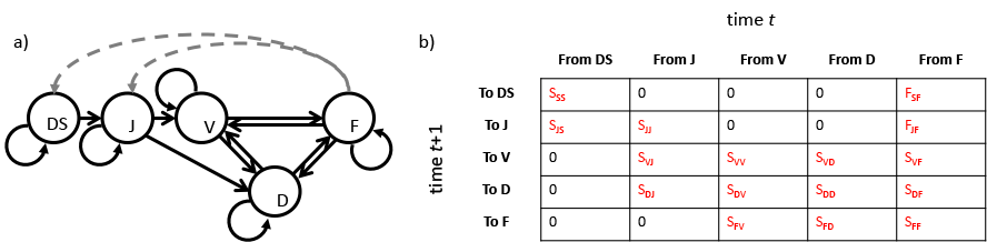
Figure 2.1 is a simple example of a stage-based life history model viewed as a life cycle graph, and its associated Lefkovitch matrix for a terrestrial orchid species, Cypripedium candidum (Shefferson et al. 2001). Each stage is shown as a node, and each transition is shown as an uni-directional arrow (a). The rates and probabilities are shown as mathematical symbols in (b), with \(S_{kj}\) denoting survival-transition probability from stage \(j\) in occasion \(t\) to stage \(k\) in occasion \(t+1\), and \(F_{kj}\) denoting the fecundity of reproductive stage \(j\) in occasion \(t\) into recruit stage \(k\) in occasion \(t+1\) in this life history.
Stages are generally defined under the assumption that they are unique moments in an organism’s life. This uniqueness is assumed to extend to the demography of the organism during its time within that stage, meaning that the stage must have a mutually exclusive set of life history characteristics. In some cases, stages are defined as developmental stages, as happens with insect instars. In other cases, stages are defined almost purely on the basis of size, as occurs with perennial herbs that may exhibit a different number of stems, leaves, and flowers in each growing season. In still other cases, stages may be defined via other characteristics, for example via age as in a Leslie MPM. As another example, the vegetative dormancy stage of some perennial herbs is defined by a lack of aboveground size, and so is characteristically not observable and may be identified in a dataset by its lack of observability (Shefferson et al. 2001).
2.1.1 Stage duration
Stages always have durations, and these durations can influence the life history model chosen. A life history model used for MPM analysis needs to employ a consistent time interval for transitions, and so stages can only be defined if they occur at roughly the time resolution of the life history model. To think about stage duration, users may wish to consider a simple model that relates the life history model to the timing of monitoring. In this model, individuals exist in some particular stage at the instance of monitoring. Monitoring happens at regular intervals, and stages are defined in ways so that their durations correspond at least to the interval between consecutive monitoring occasions. Stage transitions can then be thought of conceptually as occurring either right before the monitoring occasion (the pre-breeding model), or immediately after (the post-breeding model). To simplify analysis, we also assume that death happens at the time of transition.
Erroneous accounting of stage duration is commonplace in MPM analyses. The most common problem is that one or more stages within a life history model are characterized by different durations than other stages. Often, a stage’s actual duration is longer than acknowledged. As an example, we might wish to create a seedling stage that yields a small adult. We might initially create a simple three-stage life history in which a seed stage is followed by the seedling, and this is followed by a small adult stage, which may be capable of reproduction. Imagine, however, that the seedling stage is almost never shorter than two years, and that we have a dataset based on an annual census (i.e. our MPM will consist of annual matrices). In this circumstance, the seedling stage must be split into at least two seedling stages to force the analysis to include the correct minimum number of years to keep the organism a seedling. Failure to do so would create a model that assumes a shorter juvenile period than actually occurs, and would likely lead to biased estimates of population dynamics parameters, such as the asymptotic population growth rate.
Stage duration mismatch may also occur when actual stage durations are shorter than assumed by the model. For example, if I wish to study an insect that lives potentially up to ten years, and I employ a matrix projection model in which matrices represent one year of transition, then I cannot divide the insect instars into multiple stages if they only last several days or weeks each in succession. Instead, I would need to lump those stages together in a way that incorporates a realistic amount of instar development over the course of a single year, and use that conglomerate stage within the life history model. Alternatively, I can deal with this issue by changing the set time interval used in the MPM, making a model with a much finer time resolution (although this would require monitoring many more times than just once a year, and might require redefining other stages).
2.1.2 The process and timing of fecundity
The timing of monitoring relative to the reproductive season greatly impacts the structure of life history models. Life history models are typically categorized as either pre-breeding or post-breeding. Here, breeding refers to the production of offspring, and so a pre-breeding model assumes that monitoring is conducted immediately before the new recruits are born, while a post-breeding model assumes that the monitoring is conducted just after new recruits are born (in both cases, breeding is assumed to be seasonal). In a pre-breeding model, no organism is monitored prior to an age of approximately one year, or one of whatever time unit is being used in the study. Further, in pre-breeding models fecundity equals the production of newborns multiplied by the survival of newborns to age 1, since fecundity must take place over a full time step and the timing of the census misses both the birth event itself and the time in which the organism is a newborn (Kendall et al. 2019). In a post-breeding model, organisms are first monitored at age 0, and fecundity equals the survival of the parent from the stage/age preceding reproduction to reproduction itself, multiplied by the number of newborns produced (Kendall et al. 2019).
Population ecologists often mistakenly forget important components of fecundity because of the inherent complexity of life cycle models. Often, ecologists will estimate fecundity in pre-breeding studies erroneously as only the production of newborns, without multiplying by the survival of newborns to age 1 (Kendall et al. 2019). Ecologists working with post-breeding models often erroneously omit the survival of the parent from the stage immediately preceding reproduction, since including this term generally requires creating reproductive versions of all possible preceding stages even if, counterintuitively, they are not considered reproductive stages (Kendall et al. 2019). Both of these omissions result in biased analytical results, of which the most common problem is that population growth rate is estimated to be higher than it really is.
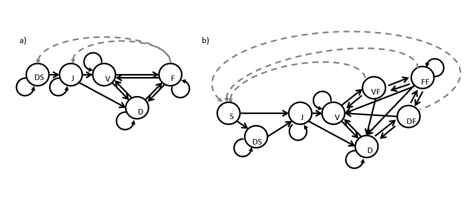
A comparison of the same system developed in pre-breeding vs. post-breeding format might help illustrate these issues. Figure 2.2 shows the same model as in figure 2.1, but given in both pre-breeding and post-breeding format. The flowering stage is the only reproductive stage in the pre-breeding model, and fecundity there is the expected number of seeds produced multiplied by either the probability of survival as a dormant seed (in production of dormant seed), or the probability of germination (in the production of juveniles). In the post-breeding model, the probability of survival from the stage preceding flowering is multiplied by the expected number of seeds, leading to a single offspring stage instead of two, and three forms of the flowering stage to deal with different expected fecundities in each case.
In monitoring studies of plant populations, the typical strategy taken is that of a pre-breeding model, in which fecundity is estimated as the production of seeds in a given year multiplied by their over-winter survival probability as seeds and their germination probability in the following year. If the life history includes seed dormancy, then it can be modeled by multiplying seed production by seed survival (which is given as the probability of maintaining seed viability from one year to the next). In more complex situations, different seed survival probabilities may be set depending on whether the seed is freshly produced or dormant within the seedbank. Added complexity can arise if there are multiple fecundity pathways, for example when clonal reproduction is also possible, or if multiple propagule stages exist, or if recruitment can yield seeds that immediately germinate as well as seeds that are dormant for one or more years. We urge users to be careful with this step, as properly defining the life history model has important implications for all analyses of population dynamics (Kendall et al. 2019).
2.1.3 Dataset and analytical influences on life history model design
Life history models can be influenced by factors seemingly external to the life history of the organism. Some of the most important considerations outside of the species’ biology include the size of the dataset, and the decision of whether to create a raw MPM or a function-based MPM. All else being equal, a larger dataset and a function-based MPM will allow more stages to be used in the life history. Assuming a dataset of fixed size, raw MPMs will include more and more zero elements as the number of stages in the life history model increases. This happens because the chance of having any individuals actually move through a specific transition decreases as the number of possible transitions increases. These increasingly common zeros can cause problems in analysis, because they suggest that some transitions are impossible when, in fact, individuals moving through them were missing just by chance. Even a transition with extremely high probability may be missing in some years just by chance. One impact of this would be the reduction of the mean transition within an element-wise mean matrix to an unrealistic level, causing both the survival probability of the associated stage and the population growth rate to be biased low.
Function-based MPMs are better able to handle large numbers of matrix elements because overparameterization is prevented by parsimonious model selection when vital rate models are determined. However, the size of the dataset influences the statistical power of these vital rate models, with smaller datasets yielding larger error associated with matrix elements. Loss of statistical power in vital rate models can lead to the loss of process variance, and can make population dynamics appear more static than they really are. In addition, adding more stages than necessary in the function-based case can create conditions in which stages themselves are estimated as having much higher survival probability than they actually do (this happens when stages that do not occur are modeled, as they are typically estimated as having trivial but non-zero probabilities of survival). The survival probability of a stage within a matrix is the column sum for that stage in a survival-transition matrix (i.e. a projection matrix without any fecundity terms). Vital rate functions generally produce non-zero values no matter what input is provided, even if sizes and conditions are entered that do not occur in the dataset, or that occur only rarely. Such situations may result in the artificial inflation of survival, and in extreme cases can result in predicted survival probability above 1.0. So, even in the function-based case, great effort needs to be taken to prevent the inclusion of too many stages, and of stages that do not actually occur in the dataset.
Chapter 6 in Morris & Doak (2002) provides a good description of techniques that may be used to define stages and to determine the exact number to use given the context imposed by a given dataset of a given size. Ellner & Rees (2006) provides a discussion of this issue within the context of integral projection model development.
Now let’s move on to create a life history model and define it in R using lefko3.
2.2 Life history model development in lefko3
The basic workflow to analysis with package lefko3 starts with the development of a life history model that encapsulates all of the appropriate life stages relevant to population dynamics. We will illustrate life history model development with the Cypripedium candidum dataset described in section 1.8.1. We will now load lefko3 and the dataset, called cypdata, after clearing memory.
The first key decision in developing a life cycle graph is to decide on which life history stages to include. This is not a simple task. We might at first believe that any clearly defined developmental stage should be its own life history stage. However, life history stages need to be defined relative to the time interval used in the MPM. They also need to be defined uniquely, and to have transitions from other stages, leading either to further life history stages or back to themselves. Finally, they also need to be defined with consideration given to the size of the dataset, since smaller datasets will allow fewer stages.
It might be easiest to begin our discussion with consideration of the function-based MPM, and what sort of life history model works best if we choose this approach. With a function-based MPM or integral projection model (IPM), there are really only two considerations that we need to be concerned about. First, which stages should be included based on a purely biological understanding of the organism’s life history and our decision on the time interval? Second, what is the range of stages and/or sizes that actually occur in the dataset and are typically encountered in nature? Let’s discuss these points in turn.
The first point - taking the biology of the organism into account - seems intuitive, but it sometimes breaks down when we consider the time interval of the study. Key issues have already been mentioned - the timing of reproduction relative to the monitoring occasion means that fecundity itself must include either newborn survival or the survival of new parents from the preceding stage, but not both. This means that the same life history might lead to a single reproductive stage if a pre-breeding model is used, or several if a post-breeding model is used (since reproduction would happen after each possible preceding stage). If newborns are propagules, such as seeds, then the same choices determine whether the first stage in the life cycle graph is a recruited juvenile (as in the pre-breeding case), or a propagule (as in the post-breeding case), or both (as in the pre-breeding case with the possibility of propagules becoming dormant). Users should take great care with this step.
The second point - identifying stages that actually occur in the dataset and that should occur typically in nature - is also important. Some stages may never be monitored, and so these will have to be included in the model but dealt with via proxy rates later. In our Cypripedium case, for example, we never monitored germinated seeds, protocorms, and seedlings, because it is essentially impossible to do so. We will include these stages in our life history model, but we will use proxy rates for their survival transitions, since we cannot use our dataset to estimate them. Conversely, there may be some stages that appear to be outliers, appearing only once and representing unusually large sizes or other unusual conditions. Such stages should not be included, because their inclusion may yield odd impacts on analysis, such as the artificial inflation of stage survival.
The choice of observable life history stages is really focused on determining which survival and fecundity transitions we have the ability to estimate given our dataset. We should develop our life cycle graph with a reasonable range of sizes and stages in mind, since we do not wish to create stages in our life cycle model that go beyond the limits of what was actually observed (models that make predictions outside of the range of data they were parameterized with have a tendency to produce erroneous and at times egregiously strange predictions). So let’s explore the range of sizes actually occurring in our dataset. There is no one variable that encapsulates the entire size of the individual in our dataset, so we will create a series of vectors that sums the numbers of sprouts that are single-flowered flowering, double-flowered flowering, and non-flowering, and use these sums as plant sizes. If we use the horizontal dataset for this purpose, then we can assess size as follows.
size.04 <- cypdata$Inf2.04 + cypdata$Inf.04 + cypdata$Veg.04
size.05 <- cypdata$Inf2.05 + cypdata$Inf.05 + cypdata$Veg.05
size.06 <- cypdata$Inf2.06 + cypdata$Inf.06 + cypdata$Veg.06
size.07 <- cypdata$Inf2.07 + cypdata$Inf.07 + cypdata$Veg.07
size.08 <- cypdata$Inf2.08 + cypdata$Inf.08 + cypdata$Veg.08
size.09 <- cypdata$Inf2.09 + cypdata$Inf.09 + cypdata$Veg.09

summary(c(size.04, size.05, size.06, size.07, size.08, size.09))
>    Min. 1st Qu.  Median    Mean 3rd Qu.    Max.    NA's
>   1.000   1.000   2.000   3.644   5.000  24.000     156
The summary shows that the smallest recorded size is a single sprout, and the largest is 24 sprouts. The many NAs are a combination of vegetative dormancy and instances of individuals being dead or simply not yet born. Given this, we might utilize the following life history model for our function-based MPMs (figure 2.3).
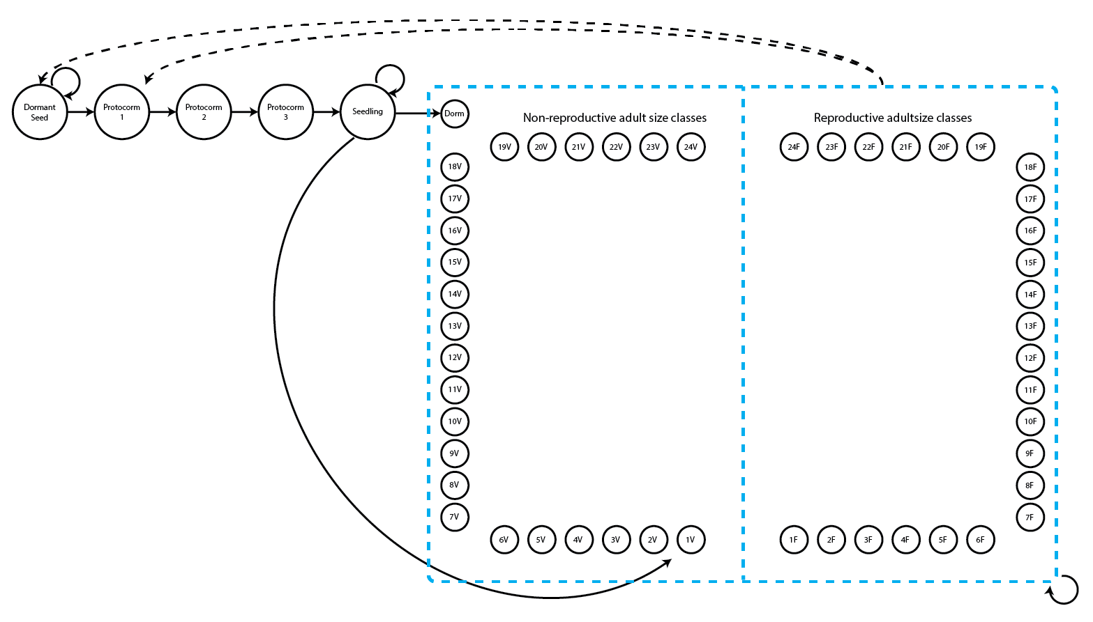
We can see a variety of transitions within this figure. The propagule and juvenile stages are the five stages in the top-left corner and have fairly simple transitions. New recruits may enter the population directly from the germination of a seed produced the previous year (Protocorm 1 stage), or they may begin as dormant seed (Dormant seed stage). Dormant seed may remain dormant, die, or germinate into the Protocorm 1 stage. Protocorms exist for up to three years without transitioning further, and individuals cannot have fewer than three years as protocorms, yielding the Protocorm 1, Protocorm 2, and Protocorm 3 stages. Protocorm 3 leads to the Seedling stage, in which the plant may persist for at least one year and potentially many years before becoming mature. Here, maturity does not really refer to reproduction per se, but rather to a morphology indistinguishable from a reproductive plant except for the lack of a flower. The first mature stage is usually either vegetative dormancy (Dorm), during which time the plant does not sprout, or a small, non-flowering adult (1V). Once in this mature portion of the life history (designated in the hashed blue box), the plant may transition among 49 mature stages, including vegetative dormancy, 1-24 shoots without flowers, or 1-24 shoots with at least one flower.
2.2.1 Building the stageframe
Now that we have our life history model, we will need to describe the life history characterizing the dataset, matching it to our analyses properly with a stageframe for our Cypripedium candidum dataset. This is a vitally important step, and most instances of errors occurring in the use of lefko3 originate from an incorrectly parameterized stageframe used in analysis. Since this analysis will be function-based, we will include all possible size classes here. If constructing raw matrices, all sizes that occur in the dataset need to be accounted for in a way that is both natural and parsimonious with respect to the numbers of individuals moving through actual transitions. If constructing function-based matrices, such as IPMs, then representative sizes at systematic increments will be satisfactory. Since size is count-based in the Cypripedium candidum case, we will use all numbers of stems that might occur from zero to the maximum in the dataset, representing the life history diagram shown in the beginning of this chapter.
To start, we will create two vectors, one showing the names of all stages in our life history model, and one showing whether the stage is included in the dataset. Both vectors utilize the same order of stages.
stagevector <- c("SD", "P1", "P2", "P3", "SL", "Dorm", "1V", "2V", "3V", "4V",
  "5V", "6V", "7V", "8V", "9V", "10V", "11V", "12V", "13V", "14V", "15V", "16V",
  "17V", "18V", "19V", "20V", "21V", "22V", "23V", "24V", "1F", "2F", "3F",
  "4F", "5F", "6F", "7F", "8F", "9F", "10F", "11F", "12F", "13F", "14F", "15F",
  "16F", "17F", "18F", "19F", "20F", "21F", "22F", "23F", "24F")
indataset <- c(0, 0, 0, 0, 0, rep(1, 49))
We included all stages in this step, and the indataset vector allows us to tell R that the first five stages ("SD", "P1", "P2", "P3", "SL") do not actually exist in the dataset. Next, we will create a few more vectors to describe the life history fully. The vectors will include the representative size (typically though not necessarily the mean or median size), reproductive status, observation status (i.e. whether it is technically possible to observe the stage, or whether the stage is essentially invisible and must be inferred to be present), and maturity status of each of these stages.
sizevector <- c(0, 0, 0, 0, 0, seq(from = 0, t = 24), seq(from = 1, to = 24))
repvector <- c(0, 0, 0, 0, 0, rep(0, 25), rep(1, 24))
obsvector <- c(0, 0, 0, 0, 0, 0, rep(1, 48))
matvector <- c(0, 0, 0, 0, 0, rep(1, 49))
Now we will create just three more vectors. The first will be a vector for status as an immature stage. While this vector might seem to be simply the logical inverse and so the mathematical complement to matvector, in truth there are cases where a stage may be both mature and immature, depending on the circumstance, and cases where a stage may actually be neither. One stage that is neither is SD, the dormant seed stage - that is marked as 0 in both cases. The second vector is a vector showing status as a propagule stage. The final vector is a comment vector, providing text descriptions of the stages.
immvector <- c(0, 1, 1, 1, 1, rep(0, 49))
propvector <- c(1, rep(0, 53))
comments <- c("Dormant seed", "Yr1 protocorm", "Yr2 protocorm", "Yr3 protocorm",
  "Seedling", "Veg dorm", "Veg adult 1 stem", "Veg adult 2 stems",
  "Veg adult 3 stems", "Veg adult 4 stems", "Veg adult 5 stems",
  "Veg adult 6 stems", "Veg adult 7 stems", "Veg adult 8 stems",
  "Veg adult 9 stems", "Veg adult 10 stems", "Veg adult 11 stems",
  "Veg adult 12 stems", "Veg adult 13 stems", "Veg adult 14 stems",
  "Veg adult 15 stems", "Veg adult 16 stems", "Veg adult 17 stems",
  "Veg adult 18 stems", "Veg adult 19 stems", "Veg adult 20 stems",
  "Veg adult 21 stems", "Veg adult 22 stems", "Veg adult 23 stems",
  "Veg adult 24 stems", "Flo adult 1 stem", "Flo adult 2 stems",
  "Flo adult 3 stems", "Flo adult 4 stems", "Flo adult 5 stems",
  "Flo adult 6 stems", "Flo adult 7 stems", "Flo adult 8 stems",
  "Flo adult 9 stems", "Flo adult 10 stems", "Flo adult 11 stems",
  "Flo adult 12 stems", "Flo adult 13 stems", "Flo adult 14 stems",
  "Flo adult 15 stems", "Flo adult 16 stems", "Flo adult 17 stems",
  "Flo adult 18 stems", "Flo adult 19 stems", "Flo adult 20 stems",
  "Flo adult 21 stems", "Flo adult 22 stems", "Flo adult 23 stems",
  "Flo adult 24 stems")
Next we will create the stageframe using the sf_create() function.
cypframe_fb <- sf_create(sizes = sizevector, stagenames = stagevector,
repstatus = repvector, obsstatus = obsvector, matstatus = matvector,
propstatus = propvector, immstatus = immvector, indataset = indataset,
comments = comments)
cypframe_fb
> stage size size_b size_c min_age max_age repstatus obsstatus propstatus
> 1 SD 0 NA NA NA NA 0 0 1
> 2 P1 0 NA NA NA NA 0 0 0
> 3 P2 0 NA NA NA NA 0 0 0
> 4 P3 0 NA NA NA NA 0 0 0
> 5 SL 0 NA NA NA NA 0 0 0
> 6 Dorm 0 NA NA NA NA 0 0 0
> 7 1V 1 NA NA NA NA 0 1 0
> 8 2V 2 NA NA NA NA 0 1 0
> 9 3V 3 NA NA NA NA 0 1 0
> 10 4V 4 NA NA NA NA 0 1 0
> 11 5V 5 NA NA NA NA 0 1 0
> 12 6V 6 NA NA NA NA 0 1 0
> 13 7V 7 NA NA NA NA 0 1 0
> 14 8V 8 NA NA NA NA 0 1 0
> 15 9V 9 NA NA NA NA 0 1 0
> 16 10V 10 NA NA NA NA 0 1 0
> 17 11V 11 NA NA NA NA 0 1 0
> 18 12V 12 NA NA NA NA 0 1 0
> 19 13V 13 NA NA NA NA 0 1 0
> 20 14V 14 NA NA NA NA 0 1 0
> 21 15V 15 NA NA NA NA 0 1 0
> 22 16V 16 NA NA NA NA 0 1 0
> 23 17V 17 NA NA NA NA 0 1 0
> 24 18V 18 NA NA NA NA 0 1 0
> 25 19V 19 NA NA NA NA 0 1 0
> 26 20V 20 NA NA NA NA 0 1 0
> 27 21V 21 NA NA NA NA 0 1 0
> 28 22V 22 NA NA NA NA 0 1 0
> 29 23V 23 NA NA NA NA 0 1 0
> 30 24V 24 NA NA NA NA 0 1 0
> 31 1F 1 NA NA NA NA 1 1 0
> 32 2F 2 NA NA NA NA 1 1 0
> 33 3F 3 NA NA NA NA 1 1 0
> 34 4F 4 NA NA NA NA 1 1 0
> immstatus matstatus indataset binhalfwidth_raw sizebin_min sizebin_max
> 1 0 0 0 0.5 -0.5 0.5
> 2 1 0 0 0.5 -0.5 0.5
> 3 1 0 0 0.5 -0.5 0.5
> 4 1 0 0 0.5 -0.5 0.5
> 5 1 0 0 0.5 -0.5 0.5
> 6 0 1 1 0.5 -0.5 0.5
> 7 0 1 1 0.5 0.5 1.5
> 8 0 1 1 0.5 1.5 2.5
> 9 0 1 1 0.5 2.5 3.5
> 10 0 1 1 0.5 3.5 4.5
> 11 0 1 1 0.5 4.5 5.5
> 12 0 1 1 0.5 5.5 6.5
> 13 0 1 1 0.5 6.5 7.5
> 14 0 1 1 0.5 7.5 8.5
> 15 0 1 1 0.5 8.5 9.5
> 16 0 1 1 0.5 9.5 10.5
> 17 0 1 1 0.5 10.5 11.5
> 18 0 1 1 0.5 11.5 12.5
> 19 0 1 1 0.5 12.5 13.5
> 20 0 1 1 0.5 13.5 14.5
> 21 0 1 1 0.5 14.5 15.5
> 22 0 1 1 0.5 15.5 16.5
> 23 0 1 1 0.5 16.5 17.5
> 24 0 1 1 0.5 17.5 18.5
> 25 0 1 1 0.5 18.5 19.5
> 26 0 1 1 0.5 19.5 20.5
> 27 0 1 1 0.5 20.5 21.5
> 28 0 1 1 0.5 21.5 22.5
> 29 0 1 1 0.5 22.5 23.5
> 30 0 1 1 0.5 23.5 24.5
> 31 0 1 1 0.5 0.5 1.5
> 32 0 1 1 0.5 1.5 2.5
> 33 0 1 1 0.5 2.5 3.5
> 34 0 1 1 0.5 3.5 4.5
> sizebin_center sizebin_width binhalfwidthb_raw sizebinb_min sizebinb_max
> 1 0 1 NA NA NA
> 2 0 1 NA NA NA
> 3 0 1 NA NA NA
> 4 0 1 NA NA NA
> 5 0 1 NA NA NA
> 6 0 1 NA NA NA
> 7 1 1 NA NA NA
> 8 2 1 NA NA NA
> 9 3 1 NA NA NA
> 10 4 1 NA NA NA
> 11 5 1 NA NA NA
> 12 6 1 NA NA NA
> 13 7 1 NA NA NA
> 14 8 1 NA NA NA
> 15 9 1 NA NA NA
> 16 10 1 NA NA NA
> 17 11 1 NA NA NA
> 18 12 1 NA NA NA
> 19 13 1 NA NA NA
> 20 14 1 NA NA NA
> 21 15 1 NA NA NA
> 22 16 1 NA NA NA
> 23 17 1 NA NA NA
> 24 18 1 NA NA NA
> 25 19 1 NA NA NA
> 26 20 1 NA NA NA
> 27 21 1 NA NA NA
> 28 22 1 NA NA NA
> 29 23 1 NA NA NA
> 30 24 1 NA NA NA
> 31 1 1 NA NA NA
> 32 2 1 NA NA NA
> 33 3 1 NA NA NA
> 34 4 1 NA NA NA
> sizebinb_center sizebinb_width binhalfwidthc_raw sizebinc_min sizebinc_max
> 1 NA NA NA NA NA
> 2 NA NA NA NA NA
> 3 NA NA NA NA NA
> 4 NA NA NA NA NA
> 5 NA NA NA NA NA
> 6 NA NA NA NA NA
> 7 NA NA NA NA NA
> 8 NA NA NA NA NA
> 9 NA NA NA NA NA
> 10 NA NA NA NA NA
> 11 NA NA NA NA NA
> 12 NA NA NA NA NA
> 13 NA NA NA NA NA
> 14 NA NA NA NA NA
> 15 NA NA NA NA NA
> 16 NA NA NA NA NA
> 17 NA NA NA NA NA
> 18 NA NA NA NA NA
> 19 NA NA NA NA NA
> 20 NA NA NA NA NA
> 21 NA NA NA NA NA
> 22 NA NA NA NA NA
> 23 NA NA NA NA NA
> 24 NA NA NA NA NA
> 25 NA NA NA NA NA
> 26 NA NA NA NA NA
> 27 NA NA NA NA NA
> 28 NA NA NA NA NA
> 29 NA NA NA NA NA
> 30 NA NA NA NA NA
> 31 NA NA NA NA NA
> 32 NA NA NA NA NA
> 33 NA NA NA NA NA
> 34 NA NA NA NA NA
> sizebinc_center sizebinc_width group comments
> 1 NA NA 0 Dormant seed
> 2 NA NA 0 Yr1 protocorm
> 3 NA NA 0 Yr2 protocorm
> 4 NA NA 0 Yr3 protocorm
> 5 NA NA 0 Seedling
> 6 NA NA 0 Veg dorm
> 7 NA NA 0 Veg adult 1 stem
> 8 NA NA 0 Veg adult 2 stems
> 9 NA NA 0 Veg adult 3 stems
> 10 NA NA 0 Veg adult 4 stems
> 11 NA NA 0 Veg adult 5 stems
> 12 NA NA 0 Veg adult 6 stems
> 13 NA NA 0 Veg adult 7 stems
> 14 NA NA 0 Veg adult 8 stems
> 15 NA NA 0 Veg adult 9 stems
> 16 NA NA 0 Veg adult 10 stems
> 17 NA NA 0 Veg adult 11 stems
> 18 NA NA 0 Veg adult 12 stems
> 19 NA NA 0 Veg adult 13 stems
> 20 NA NA 0 Veg adult 14 stems
> 21 NA NA 0 Veg adult 15 stems
> 22 NA NA 0 Veg adult 16 stems
> 23 NA NA 0 Veg adult 17 stems
> 24 NA NA 0 Veg adult 18 stems
> 25 NA NA 0 Veg adult 19 stems
> 26 NA NA 0 Veg adult 20 stems
> 27 NA NA 0 Veg adult 21 stems
> 28 NA NA 0 Veg adult 22 stems
> 29 NA NA 0 Veg adult 23 stems
> 30 NA NA 0 Veg adult 24 stems
> 31 NA NA 0 Flo adult 1 stem
> 32 NA NA 0 Flo adult 2 stems
> 33 NA NA 0 Flo adult 3 stems
> 34 NA NA 0 Flo adult 4 stems
> [ reached 'max' / getOption("max.print") -- omitted 20 rows ]
A close look at the resulting object, cypframe, shows a data frame that includes the following information in order for each stage: the stage’s name, the associated size (in terms of up to three size metrics), its minimum and maximum age of occurrence (only used if creating an age-by-stage MPM), its reproductive status, its status as an observable stage, its status as a propagule stage, its status as an immature stage, its status as a mature stage, whether it occurs in the dataset, the half-width of its size class bin, the minimum and maximum of its size class bin, the centroid of its size class bin (currently the arithmetic mean), its full size class bin width (these last five variables are given for up to three size metrics in order), the stage group that the stage belongs to, and a comments field describing the stage. Stage names and combinations of characteristics for all stages occurring in the dataset must be unique to prevent estimation errors, and the comments field may be edited to include any information deemed pertinent. Note that we did not include information on secondary and tertiary size, stage group, and the ages at which stages occur, but these may be supplied as well. We will cover these topics later in this book.
At this stage, we can build our function-based MPM. However, we might ask: How does the life history model differ if we wish to develop a raw MPM? The key difference is that we need to consider how large our dataset is, and to create only as many stages as can be routinely transitioned to and from based on the data. The life history model above in figure 2.3, for example, is not usable for a raw MPM because we have cut the size bins too finely - it is likely that in a typical year, only some of these stages will have individuals actually transitioning between them. The impact of this is that we will end up with many zero transitions that, in a sufficiently large population, should not equal zero, and this fact will force our estimates of the population growth rate lower than necessary.
To deal with this problem, we need to explore the dataset to determine a reasonable number of life history stages and where the breaks should occur between these stages. A number of means exist to do this, and users should see Caswell (2001) and Kendall et al. (2019) for good discussions of the topic. Here, we suggest plotting a size distribution and assessing a series of numbers of natural breaks using the Jenks natural breaks algorithm (Jenks 1967), or another such algorithm. Let’s take a look at a distribution plot of size to help us with this process (figure 2.4).
plot(density(c(size.04, size.05, size.06, size.07, size.08, size.09),
    na.rm = TRUE), main = "", xlab = "Size (# of sprouts)", bty = "n")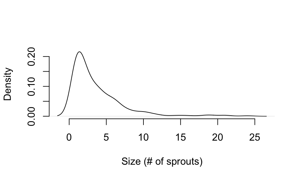
Figure 2.4: Distribution of size in Cypripedium candidum
We can see that most individuals are small, and so our size data is densest around 1-2 sprouts or so. Large individuals are rare, so we will need to make size bins wider for large plants than for small plants. Let’s try finding some natural breaks with the Jenks algorithm, separating into three, four, five, and six stages. To separate the size data into these numbers of stages, we need to identify a total of four, five, six, and seven breaks including the minimum and maximum. First, let’s install the package BAMMtools, which includes the getJenksBreaks() function.
Now let’s see where we might fit natural breaks, and how many there might need to be.
BAMMtools::getJenksBreaks(c(size.04, size.05, size.06, size.07, size.08,
    size.09), k = 4)
> [1]  1  4 12 24
BAMMtools::getJenksBreaks(c(size.04, size.05, size.06, size.07, size.08,
    size.09), k = 5)
> [1]  1  3  7 14 24
BAMMtools::getJenksBreaks(c(size.04, size.05, size.06, size.07, size.08,
    size.09), k = 6)
> [1]  1  2  4  7 14 24
BAMMtools::getJenksBreaks(c(size.04, size.05, size.06, size.07, size.08,
    size.09), k = 7)
> [1]  1  2  4  7 11 16 24
The Jenks method gives us the borders of the size classes under different numbers of stages. The first line shows a three stage model, yielding four breaks including the minimum and maximum. This model has the first stage include 1-3 sprouts, the second stage include 4-11 sprouts, and the 3rd stage include 12-24 sprouts. The fourth line is a six stage model with seven breaks shown. Given what we know about the size distribution, we will try to separate the data into five stages (one sprout, 2-3 sprouts, 4-6 sprouts, 7-13 sprouts, and 14-24 sprouts), which will result in 11 total life history stages in our life history (one dormant seed, three protocorm stages of different age, one seedling stage, one vegetatively dormant stage, and five size-classified adult stages). Here is our new life history model (figure 2.5). Note that the hashed blue box here refers to the mature stages that are actually observable in our population.
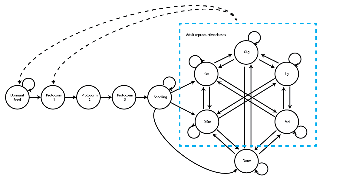
Let’s now build a stageframe using these breaks. We will build vectors designating the same kinds of information as before, plus a new vector designating the half-width of the size bins associated with each stage (the binvec vector). The default half-width is 0.5, and while we used the default for the function-based stageframe, we cannot assume the default here.
sizevector <- c(0, 0, 0, 0, 0, 0, 1, 2.5, 5, 10, 19)
stagevector <- c("SD", "P1", "P2", "P3", "SL", "Dorm", "XSm", "Sm", "Md", "Lg",
  "XLg")
repvector <- c(0, 0, 0, 0, 0, 0, 1, 1, 1, 1, 1)
obsvector <- c(0, 0, 0, 0, 0, 0, 1, 1, 1, 1, 1)
matvector <- c(0, 0, 0, 0, 0, 1, 1, 1, 1, 1, 1)
immvector <- c(0, 1, 1, 1, 1, 0, 0, 0, 0, 0, 0)
propvector <- c(1, 0, 0, 0, 0, 0, 0, 0, 0, 0, 0)
indataset <- c(0, 0, 0, 0, 0, 1, 1, 1, 1, 1, 1)
binvec <- c(0, 0, 0, 0, 0, 0.5, 0.5, 1.0, 1.5, 3.5, 5.5)

comments <- c("Dormant seed", "1st yr protocorm", "2nd yr protocorm",
  "3rd yr protocorm", "Seedling", "Dormant adult",
  "Extra small adult (1 shoot)", "Small adult (2-3 shoots)",
  "Medium adult (4-6 shoots)", "Large adult (7-13 shoots)",
  "Extra large adult (>13 shoots)")

cypframe_raw <- sf_create(sizes = sizevector, stagenames = stagevector,
  repstatus = repvector, obsstatus = obsvector, matstatus = matvector,
  propstatus = propvector, immstatus = immvector, indataset = indataset,
  binhalfwidth = binvec, comments = comments)

cypframe_raw
>    stage size size_b size_c min_age max_age repstatus obsstatus propstatus
> 1     SD  0.0     NA     NA      NA      NA         0         0          1
> 2     P1  0.0     NA     NA      NA      NA         0         0          0
> 3     P2  0.0     NA     NA      NA      NA         0         0          0
> 4     P3  0.0     NA     NA      NA      NA         0         0          0
> 5     SL  0.0     NA     NA      NA      NA         0         0          0
> 6   Dorm  0.0     NA     NA      NA      NA         0         0          0
> 7    XSm  1.0     NA     NA      NA      NA         1         1          0
> 8     Sm  2.5     NA     NA      NA      NA         1         1          0
> 9     Md  5.0     NA     NA      NA      NA         1         1          0
> 10    Lg 10.0     NA     NA      NA      NA         1         1          0
> 11   XLg 19.0     NA     NA      NA      NA         1         1          0
>    immstatus matstatus indataset binhalfwidth_raw sizebin_min sizebin_max
> 1          0         0         0              0.0         0.0         0.0
> 2          1         0         0              0.0         0.0         0.0
> 3          1         0         0              0.0         0.0         0.0
> 4          1         0         0              0.0         0.0         0.0
> 5          1         0         0              0.0         0.0         0.0
> 6          0         1         1              0.5        -0.5         0.5
> 7          0         1         1              0.5         0.5         1.5
> 8          0         1         1              1.0         1.5         3.5
> 9          0         1         1              1.5         3.5         6.5
> 10         0         1         1              3.5         6.5        13.5
> 11         0         1         1              5.5        13.5        24.5
>    sizebin_center sizebin_width binhalfwidthb_raw sizebinb_min sizebinb_max
> 1             0.0             0                NA           NA           NA
> 2             0.0             0                NA           NA           NA
> 3             0.0             0                NA           NA           NA
> 4             0.0             0                NA           NA           NA
> 5             0.0             0                NA           NA           NA
> 6             0.0             1                NA           NA           NA
> 7             1.0             1                NA           NA           NA
> 8             2.5             2                NA           NA           NA
> 9             5.0             3                NA           NA           NA
> 10           10.0             7                NA           NA           NA
> 11           19.0            11                NA           NA           NA
>    sizebinb_center sizebinb_width binhalfwidthc_raw sizebinc_min sizebinc_max
> 1               NA             NA                NA           NA           NA
> 2               NA             NA                NA           NA           NA
> 3               NA             NA                NA           NA           NA
> 4               NA             NA                NA           NA           NA
> 5               NA             NA                NA           NA           NA
> 6               NA             NA                NA           NA           NA
> 7               NA             NA                NA           NA           NA
> 8               NA             NA                NA           NA           NA
> 9               NA             NA                NA           NA           NA
> 10              NA             NA                NA           NA           NA
> 11              NA             NA                NA           NA           NA
>    sizebinc_center sizebinc_width group                       comments
> 1               NA             NA     0                   Dormant seed
> 2               NA             NA     0               1st yr protocorm
> 3               NA             NA     0               2nd yr protocorm
> 4               NA             NA     0               3rd yr protocorm
> 5               NA             NA     0                       Seedling
> 6               NA             NA     0                  Dormant adult
> 7               NA             NA     0    Extra small adult (1 shoot)
> 8               NA             NA     0       Small adult (2-3 shoots)
> 9               NA             NA     0      Medium adult (4-6 shoots)
> 10              NA             NA     0      Large adult (7-13 shoots)
> 11              NA             NA     0 Extra large adult (>13 shoots)
The above method used bin-halfwidths together with bin midpoints to define the boundaries of each bin. This generally requires some mental mathematics, and also the acceptance of the bin midpoint as the representative size. However, in reality the bin midpoint is just a representative size for the class and is not actually used in calculations. So, users may stipulate different representative sizes, as long as they supply the size minima and maxima. In the code below, we develop an alternative stageframe with the same bins used for size, but different representative sizes. Note the use of the sizemin and sizemax options. The resulting stageframe will result in the exact same MPM, whether applied to raw or function-based cases.
sizevector_alt <- c(0, 0, 0, 0, 0,    0,   1, 2.5,   5,   10, 19)
sizeminvec <-     c(0, 0, 0, 0, 0, -0.5, 0.5, 1.5, 3.5,  6.5, 13.5)
sizemaxvec <-     c(0, 0, 0, 0, 0,  0.5, 1.5, 3.5, 6.5, 13.5, 24.5)

cypframe_raw_alt <- sf_create(sizes = sizevector_alt, stagenames = stagevector,
  repstatus = repvector, obsstatus = obsvector, matstatus = matvector,
  propstatus = propvector, immstatus = immvector, indataset = indataset,
  sizemin = sizeminvec, sizemax = sizemaxvec, comments = comments)

cypframe_raw_alt
>    stage size size_b size_c min_age max_age repstatus obsstatus propstatus
> 1     SD  0.0     NA     NA      NA      NA         0         0          1
> 2     P1  0.0     NA     NA      NA      NA         0         0          0
> 3     P2  0.0     NA     NA      NA      NA         0         0          0
> 4     P3  0.0     NA     NA      NA      NA         0         0          0
> 5     SL  0.0     NA     NA      NA      NA         0         0          0
> 6   Dorm  0.0     NA     NA      NA      NA         0         0          0
> 7    XSm  1.0     NA     NA      NA      NA         1         1          0
> 8     Sm  2.5     NA     NA      NA      NA         1         1          0
> 9     Md  5.0     NA     NA      NA      NA         1         1          0
> 10    Lg 10.0     NA     NA      NA      NA         1         1          0
> 11   XLg 19.0     NA     NA      NA      NA         1         1          0
>    immstatus matstatus indataset binhalfwidth_raw sizebin_min sizebin_max
> 1          0         0         0              0.5         0.0         0.0
> 2          1         0         0              0.5         0.0         0.0
> 3          1         0         0              0.5         0.0         0.0
> 4          1         0         0              0.5         0.0         0.0
> 5          1         0         0              0.5         0.0         0.0
> 6          0         1         1              0.5        -0.5         0.5
> 7          0         1         1              0.5         0.5         1.5
> 8          0         1         1              0.5         1.5         3.5
> 9          0         1         1              0.5         3.5         6.5
> 10         0         1         1              0.5         6.5        13.5
> 11         0         1         1              0.5        13.5        24.5
>    sizebin_center sizebin_width binhalfwidthb_raw sizebinb_min sizebinb_max
> 1             0.0             0                NA           NA           NA
> 2             0.0             0                NA           NA           NA
> 3             0.0             0                NA           NA           NA
> 4             0.0             0                NA           NA           NA
> 5             0.0             0                NA           NA           NA
> 6             0.0             1                NA           NA           NA
> 7             1.0             1                NA           NA           NA
> 8             2.5             2                NA           NA           NA
> 9             5.0             3                NA           NA           NA
> 10           10.0             7                NA           NA           NA
> 11           19.0            11                NA           NA           NA
>    sizebinb_center sizebinb_width binhalfwidthc_raw sizebinc_min sizebinc_max
> 1               NA             NA                NA           NA           NA
> 2               NA             NA                NA           NA           NA
> 3               NA             NA                NA           NA           NA
> 4               NA             NA                NA           NA           NA
> 5               NA             NA                NA           NA           NA
> 6               NA             NA                NA           NA           NA
> 7               NA             NA                NA           NA           NA
> 8               NA             NA                NA           NA           NA
> 9               NA             NA                NA           NA           NA
> 10              NA             NA                NA           NA           NA
> 11              NA             NA                NA           NA           NA
>    sizebinc_center sizebinc_width group                       comments
> 1               NA             NA     0                   Dormant seed
> 2               NA             NA     0               1st yr protocorm
> 3               NA             NA     0               2nd yr protocorm
> 4               NA             NA     0               3rd yr protocorm
> 5               NA             NA     0                       Seedling
> 6               NA             NA     0                  Dormant adult
> 7               NA             NA     0    Extra small adult (1 shoot)
> 8               NA             NA     0       Small adult (2-3 shoots)
> 9               NA             NA     0      Medium adult (4-6 shoots)
> 10              NA             NA     0      Large adult (7-13 shoots)
> 11              NA             NA     0 Extra large adult (>13 shoots)
2.3 Stage classification with multiple size metrics
So far, we have seen the simplest case of stage classification with size, where each stage is defined by a mutually exclusive size bin of a single size variable. However, more complicated cases certainly exist, in which stages should be defined on the basis of multiple size variables. Let’s rethink the Cypripedium candidum example with this in mind.
In the previous two stageframes, we defined stages on the basis of the number of sprouts. However, many ecologists would argue that a flowering sprout is biologically quite different from a non-flowering sprout. Certainly, the amount of resources needed to produce a flowering sprout should be greater than that required for a non-flowering sprout. Of course, flowering sprouts actually produce offspring as well, making them demographically different from non-flowering sprouts. Further, the population actually includes an occasional, rare two-flowered sprout, as well. Can we redefine our life history model to use the numbers of non-flowering, one-flowered, and two-flowered sprouts to define stages?
To conduct this exercise, we first need to explore our data to see what combinations of different numbers of these three kinds of sprouts actually exist. We will do that using the verticalize3() function to standardize and format our demographic data first. We will describe this function in detail in the next chapter and so will not do so here. However, we will just point out that the three kinds of sprouts are input as sizeacol, sizebcol, and sizeccol in this function call, with Veg.04 designating the number of non-flowering sprouts in 2004, Inf.04 designating the number of single-flowered sprouts in 2004, and Inf2.04 designating the number of double-flowered sprouts in 2004 (other years are incorporated via the blocksize option, but more on that in the next chapter).
vert.data.check <- verticalize3(cypdata, noyears = 6, firstyear = 2004,
  patchidcol = "patch", individcol = "plantid", blocksize = 4,
  sizeacol = "Veg.04", sizebcol = "Inf.04", sizeccol = "Inf2.04",
  repstracol = "Inf.04", repstrbcol = "Inf2.04", fecacol = "Pod.04",
  censorcol = "censor", censorkeep = 1, censorRepeat = FALSE,
  NAas0 = TRUE, age_offset = 4, censor = FALSE)
summary(vert.data.check)
>      rowid          popid           patchid    individ           year2
>  Min.   : 1.00   Length:320         A: 93   Min.   : 164.0   Min.   :2004
>  1st Qu.:21.00   Class :character   B:154   1st Qu.: 391.0   1st Qu.:2005
>  Median :37.50   Mode  :character   C: 73   Median : 453.0   Median :2006
>  Mean   :38.45                              Mean   : 651.5   Mean   :2006
>  3rd Qu.:56.00                              3rd Qu.: 476.0   3rd Qu.:2007
>  Max.   :77.00                              Max.   :1560.0   Max.   :2008
>    firstseen       lastseen        obsage       obslifespan        sizea1
>  Min.   :2004   Min.   :2004   Min.   :5.000   Min.   :0.000   Min.   : 0.0
>  1st Qu.:2004   1st Qu.:2009   1st Qu.:6.000   1st Qu.:5.000   1st Qu.: 0.0
>  Median :2004   Median :2009   Median :7.000   Median :5.000   Median : 1.0
>  Mean   :2004   Mean   :2009   Mean   :6.853   Mean   :4.556   Mean   : 1.9
>  3rd Qu.:2004   3rd Qu.:2009   3rd Qu.:8.000   3rd Qu.:5.000   3rd Qu.: 3.0
>  Max.   :2008   Max.   :2009   Max.   :9.000   Max.   :5.000   Max.   :13.0
>      sizeb1            sizec1           size1added        repstra1
>  Min.   : 0.0000   Min.   :0.000000   Min.   : 0.000   Min.   : 0.0000
>  1st Qu.: 0.0000   1st Qu.:0.000000   1st Qu.: 0.000   1st Qu.: 0.0000
>  Median : 0.0000   Median :0.000000   Median : 2.000   Median : 0.0000
>  Mean   : 0.7469   Mean   :0.009375   Mean   : 2.656   Mean   : 0.7469
>  3rd Qu.: 1.0000   3rd Qu.:0.000000   3rd Qu.: 4.000   3rd Qu.: 1.0000
>  Max.   :18.0000   Max.   :1.000000   Max.   :21.000   Max.   :18.0000
>     repstrb1         repstr1added         feca1          fec1added
>  Min.   :0.000000   Min.   : 0.0000   Min.   :0.0000   Min.   :0.0000
>  1st Qu.:0.000000   1st Qu.: 0.0000   1st Qu.:0.0000   1st Qu.:0.0000
>  Median :0.000000   Median : 0.0000   Median :0.0000   Median :0.0000
>  Mean   :0.009375   Mean   : 0.7562   Mean   :0.2656   Mean   :0.2656
>  3rd Qu.:0.000000   3rd Qu.: 1.0000   3rd Qu.:0.0000   3rd Qu.:0.0000
>  Max.   :1.000000   Max.   :18.0000   Max.   :7.0000   Max.   :7.0000
>     censor1         obsstatus1       repstatus1       fecstatus1
>  Min.   :0.0000   Min.   :0.0000   Min.   :0.0000   Min.   :0.0000
>  1st Qu.:1.0000   1st Qu.:0.0000   1st Qu.:0.0000   1st Qu.:0.0000
>  Median :1.0000   Median :1.0000   Median :0.0000   Median :0.0000
>  Mean   :0.7969   Mean   :0.7469   Mean   :0.2875   Mean   :0.1344
>  3rd Qu.:1.0000   3rd Qu.:1.0000   3rd Qu.:1.0000   3rd Qu.:0.0000
>  Max.   :1.0000   Max.   :1.0000   Max.   :1.0000   Max.   :1.0000
>    matstatus1     alive1          stage1           stage1index     sizea2
>  Min.   :1    Min.   :0.0000   Length:320         Min.   :0    Min.   : 0.000
>  1st Qu.:1    1st Qu.:1.0000   Class :character   1st Qu.:0    1st Qu.: 1.000
>  Median :1    Median :1.0000   Mode  :character   Median :0    Median : 2.000
>  Mean   :1    Mean   :0.7688                      Mean   :0    Mean   : 2.416
>  3rd Qu.:1    3rd Qu.:1.0000                      3rd Qu.:0    3rd Qu.: 3.000
>  Max.   :1    Max.   :1.0000                      Max.   :0    Max.   :13.000
>      sizeb2            sizec2           size2added        repstra2
>  Min.   : 0.0000   Min.   :0.000000   Min.   : 0.000   Min.   : 0.0000
>  1st Qu.: 0.0000   1st Qu.:0.000000   1st Qu.: 1.000   1st Qu.: 0.0000
>  Median : 0.0000   Median :0.000000   Median : 2.000   Median : 0.0000
>  Mean   : 0.8969   Mean   :0.009375   Mean   : 3.322   Mean   : 0.8969
>  3rd Qu.: 1.0000   3rd Qu.:0.000000   3rd Qu.: 4.000   3rd Qu.: 1.0000
>  Max.   :18.0000   Max.   :1.000000   Max.   :24.000   Max.   :18.0000
>     repstrb2         repstr2added         feca2          fec2added
>  Min.   :0.000000   Min.   : 0.0000   Min.   :0.0000   Min.   :0.0000
>  1st Qu.:0.000000   1st Qu.: 0.0000   1st Qu.:0.0000   1st Qu.:0.0000
>  Median :0.000000   Median : 0.0000   Median :0.0000   Median :0.0000
>  Mean   :0.009375   Mean   : 0.9062   Mean   :0.2906   Mean   :0.2906
>  3rd Qu.:0.000000   3rd Qu.: 1.0000   3rd Qu.:0.0000   3rd Qu.:0.0000
>  Max.   :1.000000   Max.   :18.0000   Max.   :7.0000   Max.   :7.0000
>    obsstatus2       repstatus2       fecstatus2       matstatus2     alive2
>  Min.   :0.0000   Min.   :0.0000   Min.   :0.0000   Min.   :1    Min.   :1
>  1st Qu.:1.0000   1st Qu.:0.0000   1st Qu.:0.0000   1st Qu.:1    1st Qu.:1
>  Median :1.0000   Median :0.0000   Median :0.0000   Median :1    Median :1
>  Mean   :0.9531   Mean   :0.3688   Mean   :0.1562   Mean   :1    Mean   :1
>  3rd Qu.:1.0000   3rd Qu.:1.0000   3rd Qu.:0.0000   3rd Qu.:1    3rd Qu.:1
>  Max.   :1.0000   Max.   :1.0000   Max.   :1.0000   Max.   :1    Max.   :1
>     stage2           stage2index     sizea3           sizeb3
>  Length:320         Min.   :0    Min.   : 0.000   Min.   : 0.000
>  Class :character   1st Qu.:0    1st Qu.: 1.000   1st Qu.: 0.000
>  Mode  :character   Median :0    Median : 1.000   Median : 0.000
>                     Mean   :0    Mean   : 2.209   Mean   : 1.069
>                     3rd Qu.:0    3rd Qu.: 3.000   3rd Qu.: 1.000
>                     Max.   :0    Max.   :13.000   Max.   :18.000
>      sizec3           size3added        repstra3         repstrb3
>  Min.   :0.000000   Min.   : 0.000   Min.   : 0.000   Min.   :0.000000
>  1st Qu.:0.000000   1st Qu.: 1.000   1st Qu.: 0.000   1st Qu.:0.000000
>  Median :0.000000   Median : 2.000   Median : 0.000   Median :0.000000
>  Mean   :0.009375   Mean   : 3.288   Mean   : 1.069   Mean   :0.009375
>  3rd Qu.:0.000000   3rd Qu.: 4.000   3rd Qu.: 1.000   3rd Qu.:0.000000
>  Max.   :1.000000   Max.   :24.000   Max.   :18.000   Max.   :1.000000
>   repstr3added        feca3          fec3added        obsstatus3    repstatus3
>  Min.   : 0.000   Min.   :0.0000   Min.   :0.0000   Min.   :0.0   Min.   :0.0
>  1st Qu.: 0.000   1st Qu.:0.0000   1st Qu.:0.0000   1st Qu.:1.0   1st Qu.:0.0
>  Median : 0.000   Median :0.0000   Median :0.0000   Median :1.0   Median :0.0
>  Mean   : 1.078   Mean   :0.4562   Mean   :0.4562   Mean   :0.9   Mean   :0.4
>  3rd Qu.: 1.000   3rd Qu.:0.0000   3rd Qu.:0.0000   3rd Qu.:1.0   3rd Qu.:1.0
>  Max.   :18.000   Max.   :8.0000   Max.   :8.0000   Max.   :1.0   Max.   :1.0
>    fecstatus3       matstatus3     alive3          stage3           stage3index
>  Min.   :0.0000   Min.   :1    Min.   :0.0000   Length:320         Min.   :0
>  1st Qu.:0.0000   1st Qu.:1    1st Qu.:1.0000   Class :character   1st Qu.:0
>  Median :0.0000   Median :1    Median :1.0000   Mode  :character   Median :0
>  Mean   :0.2219   Mean   :1    Mean   :0.9469                      Mean   :0
>  3rd Qu.:0.0000   3rd Qu.:1    3rd Qu.:1.0000                      3rd Qu.:0
>  Max.   :1.0000   Max.   :1    Max.   :1.0000                      Max.   :0
The resulting object is a data frame, and we need to see what sorts of occurrences of each size actually occur within this data frame. For this purpose, we will use the xtabs() function in R’s stats package to create contingency tables of the different sizes at time \(t\).
xtabs(~ sizea2 + sizeb2 + sizec2, vert.data.check)
> , , sizec2 = 0
>
>       sizeb2
> sizea2  0  1  2  3  4  5  6  7  8 10 11 18
>     0  15 25  4  2  1  1  1  0  1  0  0  0
>     1  83 12  6  4  1  1  0  0  0  0  0  0
>     2  39  8  3  2  2  0  0  0  0  0  0  0
>     3  18  7  3  2  0  0  0  0  0  0  0  2
>     4  15  3  2  1  1  0  1  0  0  0  0  0
>     5  10  2  2  0  0  1  0  0  0  0  0  0
>     6  10  1  1  0  1  0  0  1  0  0  0  0
>     7   4  2  0  0  0  0  0  0  0  0  0  0
>     8   4  0  1  0  0  0  0  0  0  0  0  0
>     9   1  1  0  0  0  0  0  0  0  1  0  0
>     10  1  0  0  0  0  0  0  0  0  0  0  0
>     11  1  0  0  0  0  0  0  0  0  0  0  0
>     12  1  0  0  0  1  0  0  0  0  0  0  0
>     13  0  2  1  0  0  0  0  0  0  0  1  0
>
> , , sizec2 = 1
>
>       sizeb2
> sizea2  0  1  2  3  4  5  6  7  8 10 11 18
>     0   0  0  0  0  0  0  0  0  0  0  0  0
>     1   0  0  1  0  0  0  0  0  0  0  0  0
>     2   0  0  0  0  0  0  0  0  2  0  0  0
>     3   0  0  0  0  0  0  0  0  0  0  0  0
>     4   0  0  0  0  0  0  0  0  0  0  0  0
>     5   0  0  0  0  0  0  0  0  0  0  0  0
>     6   0  0  0  0  0  0  0  0  0  0  0  0
>     7   0  0  0  0  0  0  0  0  0  0  0  0
>     8   0  0  0  0  0  0  0  0  0  0  0  0
>     9   0  0  0  0  0  0  0  0  0  0  0  0
>     10  0  0  0  0  0  0  0  0  0  0  0  0
>     11  0  0  0  0  0  0  0  0  0  0  0  0
>     12  0  0  0  0  0  0  0  0  0  0  0  0
>     13  0  0  0  0  0  0  0  0  0  0  0  0
Clearly, not all size combinations are possible, and many combinations never occur. If we set up all combinations of sizes, including even a stage for 13 non-flowering sprouts and 18 single-flowered sprouts, then that stage will represent something that never actually happened in our dataset and may never happen in nature. The resulting matrices would likely include unrealistic statistics for these stages, potentially including artificially high survival. So, we will only build stages for combinations that seem likely. We might view these stages as occurring above a diagonal line running across the top contingency table, perhaps from around 11 or 12 non-flowering sprouts with no flowering sprouts, to 10 or 11 single-flowered sprouts with no non-flowering sprouts. Only the smallest two-flowered combinations will be included, as well.
sizevector.f <- c(0, 0, 0, 0, 0, 0, seq(1, 12, by = 1), seq(0, 9, by = 1),
seq(0, 8, by = 1), seq(0, 7, by = 1), seq(0, 6, by = 1), seq(0, 5, by = 1),
seq(0, 4, by = 1), seq(0, 3, by = 1), 0, 1, 2, 0, 1, 0,
0, 0, 1, 0)
sizebvector.f <- c(0, 0, 0, 0, 0, 0, rep(0, 12), rep(1, 10), rep(2, 9),
rep(3, 8), rep(4, 7), rep(5, 6), rep(6, 5), rep(7, 4), rep(8, 3), 9, 9, 10,
0, 1, 1, 2)
sizecvector.f <- c(0, 0, 0, 0, 0, 0, rep(0, 12), rep(0, 10), rep(0, 9),
rep(0, 8), rep(0, 7), rep(0, 6), rep(0, 5), rep(0, 4), 0, 0, 0, 0, 0, 0,
1, 1, 1, 1)
stagevector.f <- c("DS", "P1", "P2", "P3", "Sdl", "Dorm", "1V 0I 0D",
"2V 0I 0D", "3V 0I 0D", "4V 0I 0D", "5V 0I 0D", "6V 0I 0D", "7V 0I 0D",
"8V 0I 0D", "9V 0I 0D", "10V 0I 0D", "11V 0I 0D", "12V 0I 0D", "V0 1I 0D",
"1V 1I 0D", "2V 1I 0D", "3V 1I 0D", "4V 1I 0D", "5V 1I 0D", "6V 1I 0D",
"7V 1I 0D", "8V 1I 0D", "9V 1I 0D", "V0 2I 0D", "1V 2I 0D", "2V 2I 0D",
"3V 2I 0D", "4V 2I 0D", "5V 2I 0D", "6V 2I 0D", "7V 2I 0D", "8V 2I 0D",
"V0 3I 0D", "1V 3I 0D", "2V 3I 0D", "3V 3I 0D", "4V 3I 0D", "5V 3I 0D",
"6V 3I 0D", "7V 3I 0D", "V0 4I 0D", "1V 4I 0D", "2V 4I 0D", "3V 4I 0D",
"4V 4I 0D", "5V 4I 0D", "6V 4I 0D", "V0 5I 0D", "1V 5I 0D", "2V 5I 0D",
"3V 5I 0D", "4V 5I 0D", "5V 5I 0D", "V0 6I 0D", "1V 6I 0D", "2V 6I 0D",
"3V 6I 0D", "4V 6I 0D", "V0 7I 0D", "1V 7I 0D", "2V 7I 0D", "3V 7I 0D",
"V0 8I 0D", "1V 8I 0D", "2V 8I 0D", "V0 9I 0D", "1V 9I 0D", "V0 10I 0D",
"V0 0I 1D", "V0 1I 1D", "1V 1I 1D", "V0 2I 1D")
repvector.f <- c(0, 0, 0, 0, 0, rep(0, 13), rep(1, 59))
obsvector.f <- c(0, 0, 0, 0, 0, 0, rep(1, 71))
matvector.f <- c(0, 0, 0, 0, 0, rep(1, 72))
immvector.f <- c(0, 1, 1, 1, 1, rep(0, 72))
propvector.f <- c(1, rep(0, 76))
indataset.f <- c(0, 0, 0, 0, 0, rep(1, 72))
binvec.f <- c(0, 0, 0, 0, 0, rep(0.5, 72))
binbvec.f <- c(0, 0, 0, 0, 0, rep(0.5, 72))
bincvec.f <- c(0, 0, 0, 0, 0, rep(0.5, 72))
vertframe.3f <- sf_create(sizes = sizevector.f, sizesb = sizebvector.f,
sizesc = sizecvector.f, stagenames = stagevector.f, repstatus = repvector.f,
obsstatus = obsvector.f, propstatus = propvector.f, immstatus = immvector.f,
matstatus = matvector.f, indataset = indataset.f, binhalfwidth = binvec.f,
binhalfwidthb = binbvec.f, binhalfwidthc = bincvec.f)
vertframe.3f
> stage size size_b size_c min_age max_age repstatus obsstatus propstatus
> 1 DS 0 0 0 NA NA 0 0 1
> 2 P1 0 0 0 NA NA 0 0 0
> 3 P2 0 0 0 NA NA 0 0 0
> 4 P3 0 0 0 NA NA 0 0 0
> 5 Sdl 0 0 0 NA NA 0 0 0
> 6 Dorm 0 0 0 NA NA 0 0 0
> 7 1V 0I 0D 1 0 0 NA NA 0 1 0
> 8 2V 0I 0D 2 0 0 NA NA 0 1 0
> 9 3V 0I 0D 3 0 0 NA NA 0 1 0
> 10 4V 0I 0D 4 0 0 NA NA 0 1 0
> 11 5V 0I 0D 5 0 0 NA NA 0 1 0
> 12 6V 0I 0D 6 0 0 NA NA 0 1 0
> 13 7V 0I 0D 7 0 0 NA NA 0 1 0
> 14 8V 0I 0D 8 0 0 NA NA 0 1 0
> 15 9V 0I 0D 9 0 0 NA NA 0 1 0
> 16 10V 0I 0D 10 0 0 NA NA 0 1 0
> 17 11V 0I 0D 11 0 0 NA NA 0 1 0
> 18 12V 0I 0D 12 0 0 NA NA 0 1 0
> 19 V0 1I 0D 0 1 0 NA NA 1 1 0
> 20 1V 1I 0D 1 1 0 NA NA 1 1 0
> 21 2V 1I 0D 2 1 0 NA NA 1 1 0
> 22 3V 1I 0D 3 1 0 NA NA 1 1 0
> 23 4V 1I 0D 4 1 0 NA NA 1 1 0
> 24 5V 1I 0D 5 1 0 NA NA 1 1 0
> 25 6V 1I 0D 6 1 0 NA NA 1 1 0
> 26 7V 1I 0D 7 1 0 NA NA 1 1 0
> 27 8V 1I 0D 8 1 0 NA NA 1 1 0
> 28 9V 1I 0D 9 1 0 NA NA 1 1 0
> 29 V0 2I 0D 0 2 0 NA NA 1 1 0
> 30 1V 2I 0D 1 2 0 NA NA 1 1 0
> 31 2V 2I 0D 2 2 0 NA NA 1 1 0
> 32 3V 2I 0D 3 2 0 NA NA 1 1 0
> 33 4V 2I 0D 4 2 0 NA NA 1 1 0
> 34 5V 2I 0D 5 2 0 NA NA 1 1 0
> immstatus matstatus indataset binhalfwidth_raw sizebin_min sizebin_max
> 1 0 0 0 0.0 0.0 0.0
> 2 1 0 0 0.0 0.0 0.0
> 3 1 0 0 0.0 0.0 0.0
> 4 1 0 0 0.0 0.0 0.0
> 5 1 0 0 0.0 0.0 0.0
> 6 0 1 1 0.5 -0.5 0.5
> 7 0 1 1 0.5 0.5 1.5
> 8 0 1 1 0.5 1.5 2.5
> 9 0 1 1 0.5 2.5 3.5
> 10 0 1 1 0.5 3.5 4.5
> 11 0 1 1 0.5 4.5 5.5
> 12 0 1 1 0.5 5.5 6.5
> 13 0 1 1 0.5 6.5 7.5
> 14 0 1 1 0.5 7.5 8.5
> 15 0 1 1 0.5 8.5 9.5
> 16 0 1 1 0.5 9.5 10.5
> 17 0 1 1 0.5 10.5 11.5
> 18 0 1 1 0.5 11.5 12.5
> 19 0 1 1 0.5 -0.5 0.5
> 20 0 1 1 0.5 0.5 1.5
> 21 0 1 1 0.5 1.5 2.5
> 22 0 1 1 0.5 2.5 3.5
> 23 0 1 1 0.5 3.5 4.5
> 24 0 1 1 0.5 4.5 5.5
> 25 0 1 1 0.5 5.5 6.5
> 26 0 1 1 0.5 6.5 7.5
> 27 0 1 1 0.5 7.5 8.5
> 28 0 1 1 0.5 8.5 9.5
> 29 0 1 1 0.5 -0.5 0.5
> 30 0 1 1 0.5 0.5 1.5
> 31 0 1 1 0.5 1.5 2.5
> 32 0 1 1 0.5 2.5 3.5
> 33 0 1 1 0.5 3.5 4.5
> 34 0 1 1 0.5 4.5 5.5
> sizebin_center sizebin_width binhalfwidthb_raw sizebinb_min sizebinb_max
> 1 0 0 0.0 0.0 0.0
> 2 0 0 0.0 0.0 0.0
> 3 0 0 0.0 0.0 0.0
> 4 0 0 0.0 0.0 0.0
> 5 0 0 0.0 0.0 0.0
> 6 0 1 0.5 -0.5 0.5
> 7 1 1 0.5 -0.5 0.5
> 8 2 1 0.5 -0.5 0.5
> 9 3 1 0.5 -0.5 0.5
> 10 4 1 0.5 -0.5 0.5
> 11 5 1 0.5 -0.5 0.5
> 12 6 1 0.5 -0.5 0.5
> 13 7 1 0.5 -0.5 0.5
> 14 8 1 0.5 -0.5 0.5
> 15 9 1 0.5 -0.5 0.5
> 16 10 1 0.5 -0.5 0.5
> 17 11 1 0.5 -0.5 0.5
> 18 12 1 0.5 -0.5 0.5
> 19 0 1 0.5 0.5 1.5
> 20 1 1 0.5 0.5 1.5
> 21 2 1 0.5 0.5 1.5
> 22 3 1 0.5 0.5 1.5
> 23 4 1 0.5 0.5 1.5
> 24 5 1 0.5 0.5 1.5
> 25 6 1 0.5 0.5 1.5
> 26 7 1 0.5 0.5 1.5
> 27 8 1 0.5 0.5 1.5
> 28 9 1 0.5 0.5 1.5
> 29 0 1 0.5 1.5 2.5
> 30 1 1 0.5 1.5 2.5
> 31 2 1 0.5 1.5 2.5
> 32 3 1 0.5 1.5 2.5
> 33 4 1 0.5 1.5 2.5
> 34 5 1 0.5 1.5 2.5
> sizebinb_center sizebinb_width binhalfwidthc_raw sizebinc_min sizebinc_max
> 1 0 0 0.0 0.0 0.0
> 2 0 0 0.0 0.0 0.0
> 3 0 0 0.0 0.0 0.0
> 4 0 0 0.0 0.0 0.0
> 5 0 0 0.0 0.0 0.0
> 6 0 1 0.5 -0.5 0.5
> 7 0 1 0.5 -0.5 0.5
> 8 0 1 0.5 -0.5 0.5
> 9 0 1 0.5 -0.5 0.5
> 10 0 1 0.5 -0.5 0.5
> 11 0 1 0.5 -0.5 0.5
> 12 0 1 0.5 -0.5 0.5
> 13 0 1 0.5 -0.5 0.5
> 14 0 1 0.5 -0.5 0.5
> 15 0 1 0.5 -0.5 0.5
> 16 0 1 0.5 -0.5 0.5
> 17 0 1 0.5 -0.5 0.5
> 18 0 1 0.5 -0.5 0.5
> 19 1 1 0.5 -0.5 0.5
> 20 1 1 0.5 -0.5 0.5
> 21 1 1 0.5 -0.5 0.5
> 22 1 1 0.5 -0.5 0.5
> 23 1 1 0.5 -0.5 0.5
> 24 1 1 0.5 -0.5 0.5
> 25 1 1 0.5 -0.5 0.5
> 26 1 1 0.5 -0.5 0.5
> 27 1 1 0.5 -0.5 0.5
> 28 1 1 0.5 -0.5 0.5
> 29 2 1 0.5 -0.5 0.5
> 30 2 1 0.5 -0.5 0.5
> 31 2 1 0.5 -0.5 0.5
> 32 2 1 0.5 -0.5 0.5
> 33 2 1 0.5 -0.5 0.5
> 34 2 1 0.5 -0.5 0.5
> sizebinc_center sizebinc_width group comments
> 1 0 0 0 No description
> 2 0 0 0 No description
> 3 0 0 0 No description
> 4 0 0 0 No description
> 5 0 0 0 No description
> 6 0 1 0 No description
> 7 0 1 0 No description
> 8 0 1 0 No description
> 9 0 1 0 No description
> 10 0 1 0 No description
> 11 0 1 0 No description
> 12 0 1 0 No description
> 13 0 1 0 No description
> 14 0 1 0 No description
> 15 0 1 0 No description
> 16 0 1 0 No description
> 17 0 1 0 No description
> 18 0 1 0 No description
> 19 0 1 0 No description
> 20 0 1 0 No description
> 21 0 1 0 No description
> 22 0 1 0 No description
> 23 0 1 0 No description
> 24 0 1 0 No description
> 25 0 1 0 No description
> 26 0 1 0 No description
> 27 0 1 0 No description
> 28 0 1 0 No description
> 29 0 1 0 No description
> 30 0 1 0 No description
> 31 0 1 0 No description
> 32 0 1 0 No description
> 33 0 1 0 No description
> 34 0 1 0 No description
> [ reached 'max' / getOption("max.print") -- omitted 43 rows ]The result is our biggest stageframe yet, but a realistic one that we will go back to later.
2.4 Automating the creation of large numbers of stages
There may be times when we wish to create extremely large life history models, with many tens of life stages. For example, users wishing to develop IPMs may wish to create stageframes with over 100 stages, most of which would differ only by size. Developing stageframes for these situations can take some time and effort. Fortunately, lefko3 includes a method to make this quick and easy.
The key innovation is to use an option in function sf_create() that allows us to set the minimum and maximum sizes for a group of stages that are alike in every way except for size. A further option can set the number of total size classes to fit within these bounds. Let’s try an example, using the Cypripedium candidum case.
The size metrics that we will use in the Cypripedium candidum dataset are all count variables. However, let us pretend that the total number of sprouts is actually a continuous, quantitative variable with a minimum of 1 and a maximum of 23. If we wished to create 100 stages within these bounds, we could do so by identifying the minimum and maximum size values with the "ipm" marker in the stage names. The ipmbins option defaults to 100, but let us say so explicitly here. We will then look at just a few key variables in the resulting stageframe.
sizevector <- c(0, 0, 0, 0, 0, 0, 1, 23)
stagevector <- c("SD", "P1", "P2", "P3", "SL", "Dorm", "ipm", "ipm")
repvector <- c(0, 0, 0, 0, 0, 0, 1, 1)
obsvector <- c(0, 0, 0, 0, 0, 0, 1, 1)
matvector <- c(0, 0, 0, 0, 0, 1, 1, 1)
immvector <- c(0, 1, 1, 1, 1, 0, 0, 0)
propvector <- c(1, 0, 0, 0, 0, 0, 0, 0)
indataset <- c(0, 0, 0, 0, 0, 1, 1, 1)
binvec <- c(0, 0, 0, 0, 0, 0.5, NA, NA)

cypframe_ipm <- sf_create(sizes = sizevector, stagenames = stagevector,
  repstatus = repvector, obsstatus = obsvector, matstatus = matvector,
  propstatus = propvector, immstatus = immvector, indataset = indataset,
  binhalfwidth = binvec, ipmbins = 100)
> Warning: Values supplied in vectors sizemin, sizemax, and binhalfwidth will be overwritten for ipm bins.

cypframe_ipm[,c("stage", "size", "sizebin_min", "sizebin_max")]
>            stage  size sizebin_min sizebin_max
> 1             SD  0.00        0.00        0.00
> 2             P1  0.00        0.00        0.00
> 3             P2  0.00        0.00        0.00
> 4             P3  0.00        0.00        0.00
> 5             SL  0.00        0.00        0.00
> 6           Dorm  0.00       -0.50        0.50
> 7   sza_1.1100_0  1.11        1.00        1.22
> 8   sza_1.3300_0  1.33        1.22        1.44
> 9   sza_1.5500_0  1.55        1.44        1.66
> 10  sza_1.7700_0  1.77        1.66        1.88
> 11  sza_1.9900_0  1.99        1.88        2.10
> 12  sza_2.2100_0  2.21        2.10        2.32
> 13  sza_2.4300_0  2.43        2.32        2.54
> 14  sza_2.6500_0  2.65        2.54        2.76
> 15  sza_2.8700_0  2.87        2.76        2.98
> 16  sza_3.0900_0  3.09        2.98        3.20
> 17  sza_3.3100_0  3.31        3.20        3.42
> 18  sza_3.5300_0  3.53        3.42        3.64
> 19  sza_3.7500_0  3.75        3.64        3.86
> 20  sza_3.9700_0  3.97        3.86        4.08
> 21  sza_4.1900_0  4.19        4.08        4.30
> 22  sza_4.4100_0  4.41        4.30        4.52
> 23  sza_4.6300_0  4.63        4.52        4.74
> 24  sza_4.8500_0  4.85        4.74        4.96
> 25  sza_5.0700_0  5.07        4.96        5.18
> 26  sza_5.2900_0  5.29        5.18        5.40
> 27  sza_5.5100_0  5.51        5.40        5.62
> 28  sza_5.7300_0  5.73        5.62        5.84
> 29  sza_5.9500_0  5.95        5.84        6.06
> 30  sza_6.1700_0  6.17        6.06        6.28
> 31  sza_6.3900_0  6.39        6.28        6.50
> 32  sza_6.6100_0  6.61        6.50        6.72
> 33  sza_6.8300_0  6.83        6.72        6.94
> 34  sza_7.0500_0  7.05        6.94        7.16
> 35  sza_7.2700_0  7.27        7.16        7.38
> 36  sza_7.4900_0  7.49        7.38        7.60
> 37  sza_7.7100_0  7.71        7.60        7.82
> 38  sza_7.9300_0  7.93        7.82        8.04
> 39  sza_8.1500_0  8.15        8.04        8.26
> 40  sza_8.3700_0  8.37        8.26        8.48
> 41  sza_8.5900_0  8.59        8.48        8.70
> 42  sza_8.8100_0  8.81        8.70        8.92
> 43  sza_9.0300_0  9.03        8.92        9.14
> 44  sza_9.2500_0  9.25        9.14        9.36
> 45  sza_9.4700_0  9.47        9.36        9.58
> 46  sza_9.6900_0  9.69        9.58        9.80
> 47  sza_9.9100_0  9.91        9.80       10.02
> 48  sza_10.130_0 10.13       10.02       10.24
> 49  sza_10.350_0 10.35       10.24       10.46
> 50  sza_10.570_0 10.57       10.46       10.68
> 51  sza_10.790_0 10.79       10.68       10.90
> 52  sza_11.010_0 11.01       10.90       11.12
> 53  sza_11.230_0 11.23       11.12       11.34
> 54  sza_11.450_0 11.45       11.34       11.56
> 55  sza_11.670_0 11.67       11.56       11.78
> 56  sza_11.890_0 11.89       11.78       12.00
> 57  sza_12.110_0 12.11       12.00       12.22
> 58  sza_12.330_0 12.33       12.22       12.44
> 59  sza_12.550_0 12.55       12.44       12.66
> 60  sza_12.770_0 12.77       12.66       12.88
> 61  sza_12.990_0 12.99       12.88       13.10
> 62  sza_13.210_0 13.21       13.10       13.32
> 63  sza_13.430_0 13.43       13.32       13.54
> 64  sza_13.650_0 13.65       13.54       13.76
> 65  sza_13.870_0 13.87       13.76       13.98
> 66  sza_14.090_0 14.09       13.98       14.20
> 67  sza_14.310_0 14.31       14.20       14.42
> 68  sza_14.530_0 14.53       14.42       14.64
> 69  sza_14.750_0 14.75       14.64       14.86
> 70  sza_14.970_0 14.97       14.86       15.08
> 71  sza_15.190_0 15.19       15.08       15.30
> 72  sza_15.410_0 15.41       15.30       15.52
> 73  sza_15.630_0 15.63       15.52       15.74
> 74  sza_15.850_0 15.85       15.74       15.96
> 75  sza_16.070_0 16.07       15.96       16.18
> 76  sza_16.290_0 16.29       16.18       16.40
> 77  sza_16.510_0 16.51       16.40       16.62
> 78  sza_16.730_0 16.73       16.62       16.84
> 79  sza_16.950_0 16.95       16.84       17.06
> 80  sza_17.170_0 17.17       17.06       17.28
> 81  sza_17.390_0 17.39       17.28       17.50
> 82  sza_17.610_0 17.61       17.50       17.72
> 83  sza_17.830_0 17.83       17.72       17.94
> 84  sza_18.050_0 18.05       17.94       18.16
> 85  sza_18.270_0 18.27       18.16       18.38
> 86  sza_18.490_0 18.49       18.38       18.60
> 87  sza_18.710_0 18.71       18.60       18.82
> 88  sza_18.930_0 18.93       18.82       19.04
> 89  sza_19.150_0 19.15       19.04       19.26
> 90  sza_19.370_0 19.37       19.26       19.48
> 91  sza_19.590_0 19.59       19.48       19.70
> 92  sza_19.810_0 19.81       19.70       19.92
> 93  sza_20.030_0 20.03       19.92       20.14
> 94  sza_20.250_0 20.25       20.14       20.36
> 95  sza_20.470_0 20.47       20.36       20.58
> 96  sza_20.690_0 20.69       20.58       20.80
> 97  sza_20.910_0 20.91       20.80       21.02
> 98  sza_21.130_0 21.13       21.02       21.24
> 99  sza_21.350_0 21.35       21.24       21.46
> 100 sza_21.570_0 21.57       21.46       21.68
> 101 sza_21.790_0 21.79       21.68       21.90
> 102 sza_22.010_0 22.01       21.90       22.12
> 103 sza_22.230_0 22.23       22.12       22.34
> 104 sza_22.450_0 22.45       22.34       22.56
> 105 sza_22.670_0 22.67       22.56       22.78
> 106 sza_22.890_0 22.89       22.78       23.00
We see that we have created a total of 106 stages - five early-life stages, and then vegetative dormancy followed by 100 stages that were developed automatically. These stages have size bins that do not overlap with neighboring sizes, and cover all possible sizes in the range.
We will see more uses of this approach in chapter 7 on integral projection models. However, it is important to point out that this approach can be used for multiple groups of stages, each with its own unique combinations of stage characteristics and with their own size minima and maxima. This approach can also be used in multiple size classification scenarios. More on this later.
2.5 Advanced stageframe creation
Finally, users who have developed stageframes and wish for extra flexibility without the error-checking functions of function sf_create() may also use function sf_skeleton() to create a skeleton stageframe to edit by hand. For example, imagine that we wished to create a raw MPM stageframe this way, using the same values as before. Let’s first create the skeleton stageframe itself.
alt_sf <- sf_skeleton(11)
alt_sf
>       stage size size_b size_c min_age max_age repstatus obsstatus propstatus
> 1   stage 1    1      0      0       0       0         0         1          0
> 2   stage 2    2      0      0       0       0         0         1          0
> 3   stage 3    3      0      0       0       0         0         1          0
> 4   stage 4    4      0      0       0       0         0         1          0
> 5   stage 5    5      0      0       0       0         0         1          0
> 6   stage 6    6      0      0       0       0         0         1          0
> 7   stage 7    7      0      0       0       0         0         1          0
> 8   stage 8    8      0      0       0       0         0         1          0
> 9   stage 9    9      0      0       0       0         0         1          0
> 10 stage 10   10      0      0       0       0         0         1          0
> 11 stage 11   11      0      0       0       0         0         1          0
>    immstatus matstatus indataset binhalfwidth_raw sizebin_min sizebin_max
> 1          0         0         1              0.5           0           0
> 2          0         0         1              0.5           0           0
> 3          0         0         1              0.5           0           0
> 4          0         0         1              0.5           0           0
> 5          0         0         1              0.5           0           0
> 6          0         0         1              0.5           0           0
> 7          0         0         1              0.5           0           0
> 8          0         0         1              0.5           0           0
> 9          0         0         1              0.5           0           0
> 10         0         0         1              0.5           0           0
> 11         0         0         1              0.5           0           0
>    sizebin_center sizebin_width binhalfwidthb_raw sizebinb_min sizebinb_max
> 1               1             1                 0            0            0
> 2               2             1                 0            0            0
> 3               3             1                 0            0            0
> 4               4             1                 0            0            0
> 5               5             1                 0            0            0
> 6               6             1                 0            0            0
> 7               7             1                 0            0            0
> 8               8             1                 0            0            0
> 9               9             1                 0            0            0
> 10             10             1                 0            0            0
> 11             11             1                 0            0            0
>    sizebinb_center sizebinb_width binhalfwidthc_raw sizebinc_min sizebinc_max
> 1                0              0                 0            0            0
> 2                0              0                 0            0            0
> 3                0              0                 0            0            0
> 4                0              0                 0            0            0
> 5                0              0                 0            0            0
> 6                0              0                 0            0            0
> 7                0              0                 0            0            0
> 8                0              0                 0            0            0
> 9                0              0                 0            0            0
> 10               0              0                 0            0            0
> 11               0              0                 0            0            0
>    sizebinc_center sizebinc_width group         comments
> 1                0              0     0  stage 1 comment
> 2                0              0     0  stage 2 comment
> 3                0              0     0  stage 3 comment
> 4                0              0     0  stage 4 comment
> 5                0              0     0  stage 5 comment
> 6                0              0     0  stage 6 comment
> 7                0              0     0  stage 7 comment
> 8                0              0     0  stage 8 comment
> 9                0              0     0  stage 9 comment
> 10               0              0     0 stage 10 comment
> 11               0              0     0 stage 11 comment
The resulting object is generally full of standard default values that need to be edited. Let’s edit the vectors as necessary, as below.
alt_sf$size <- c(0, 0, 0, 0, 0, 0, 1, 2.5, 5, 10, 19)
alt_sf$stage <- c("SD", "P1", "P2", "P3", "SL", "Dorm", "XSm", "Sm", "Md", "Lg",
  "XLg")
alt_sf$repstatus <- c(0, 0, 0, 0, 0, 0, 1, 1, 1, 1, 1)
alt_sf$obsstatus <- c(0, 0, 0, 0, 0, 0, 1, 1, 1, 1, 1)
alt_sf$matstatus <- c(0, 0, 0, 0, 0, 1, 1, 1, 1, 1, 1)
alt_sf$immstatus <- c(0, 1, 1, 1, 1, 0, 0, 0, 0, 0, 0)
alt_sf$propstatus <- c(1, 0, 0, 0, 0, 0, 0, 0, 0, 0, 0)
alt_sf$indataset <- c(0, 0, 0, 0, 0, 1, 1, 1, 1, 1, 1)
alt_sf$binhalfwidth_raw <- c(0, 0, 0, 0, 0, 0.5, 0.5, 1.0, 1.5, 3.5, 5.5)
alt_sf$sizebin_min <- alt_sf$size - alt_sf$binhalfwidth_raw
alt_sf$sizebin_max <- alt_sf$size + alt_sf$binhalfwidth_raw
alt_sf$sizebin_center <- alt_sf$size

alt_sf$comments <- c("Dormant seed", "1st yr protocorm", "2nd yr protocorm",
  "3rd yr protocorm", "Seedling", "Dormant adult",
  "Extra small adult (1 shoot)", "Small adult (2-4 shoots)",
  "Medium adult (5-7 shoots)", "Large adult (8-14 shoots)",
  "Extra large adult (>14 shoots)")

alt_sf
>    stage size size_b size_c min_age max_age repstatus obsstatus propstatus
> 1     SD  0.0      0      0       0       0         0         0          1
> 2     P1  0.0      0      0       0       0         0         0          0
> 3     P2  0.0      0      0       0       0         0         0          0
> 4     P3  0.0      0      0       0       0         0         0          0
> 5     SL  0.0      0      0       0       0         0         0          0
> 6   Dorm  0.0      0      0       0       0         0         0          0
> 7    XSm  1.0      0      0       0       0         1         1          0
> 8     Sm  2.5      0      0       0       0         1         1          0
> 9     Md  5.0      0      0       0       0         1         1          0
> 10    Lg 10.0      0      0       0       0         1         1          0
> 11   XLg 19.0      0      0       0       0         1         1          0
>    immstatus matstatus indataset binhalfwidth_raw sizebin_min sizebin_max
> 1          0         0         0              0.0         0.0         0.0
> 2          1         0         0              0.0         0.0         0.0
> 3          1         0         0              0.0         0.0         0.0
> 4          1         0         0              0.0         0.0         0.0
> 5          1         0         0              0.0         0.0         0.0
> 6          0         1         1              0.5        -0.5         0.5
> 7          0         1         1              0.5         0.5         1.5
> 8          0         1         1              1.0         1.5         3.5
> 9          0         1         1              1.5         3.5         6.5
> 10         0         1         1              3.5         6.5        13.5
> 11         0         1         1              5.5        13.5        24.5
>    sizebin_center sizebin_width binhalfwidthb_raw sizebinb_min sizebinb_max
> 1             0.0             1                 0            0            0
> 2             0.0             1                 0            0            0
> 3             0.0             1                 0            0            0
> 4             0.0             1                 0            0            0
> 5             0.0             1                 0            0            0
> 6             0.0             1                 0            0            0
> 7             1.0             1                 0            0            0
> 8             2.5             1                 0            0            0
> 9             5.0             1                 0            0            0
> 10           10.0             1                 0            0            0
> 11           19.0             1                 0            0            0
>    sizebinb_center sizebinb_width binhalfwidthc_raw sizebinc_min sizebinc_max
> 1                0              0                 0            0            0
> 2                0              0                 0            0            0
> 3                0              0                 0            0            0
> 4                0              0                 0            0            0
> 5                0              0                 0            0            0
> 6                0              0                 0            0            0
> 7                0              0                 0            0            0
> 8                0              0                 0            0            0
> 9                0              0                 0            0            0
> 10               0              0                 0            0            0
> 11               0              0                 0            0            0
>    sizebinc_center sizebinc_width group                       comments
> 1                0              0     0                   Dormant seed
> 2                0              0     0               1st yr protocorm
> 3                0              0     0               2nd yr protocorm
> 4                0              0     0               3rd yr protocorm
> 5                0              0     0                       Seedling
> 6                0              0     0                  Dormant adult
> 7                0              0     0    Extra small adult (1 shoot)
> 8                0              0     0       Small adult (2-4 shoots)
> 9                0              0     0      Medium adult (5-7 shoots)
> 10               0              0     0      Large adult (8-14 shoots)
> 11               0              0     0 Extra large adult (>14 shoots)
At this point, we have five stageframes and can move ahead to standardizing and formatting our demographic datasets and creating some MPMs with them. There are further options that we can use to develop more complicated life history models, including the use of stage grouping to help properly format MPMs, and the designation of ages for each stage for use in age-by-stage MPMs. We will explore such issues in later chapters. For further information on life history model development, see chapters 3 and 4 in Caswell (2001) for a good treatment useful for beginners. We also note Kendall et al. (2019) as a good reference detailing common problems in MPM construction and how to avoid them through proper development and operationalization of life history models. Beissinger & Westphal (1998), Wardle (1998), and Salguero-Gómez & Casper (2010) provide good discussions of the proper application of life history models to understand population dynamics through the MPM approach.
2.6 Points to remember
- All MPMs and IPMs require appropriate and carefully thought out models of the life history of the organism.
- Good life history models require appropriately defined life history stages, which are defined not simply by their size and reproductive characteristics, but also by their stage duration, their relationships to other stages, by the actual numbers of different combinations of life history characteristics occurring in the dataset, and by the choice of raw vs. function-based MPM.
- Function
sf_create()will develop a data frame identifying each stage in the life history model, and this data frame will be used at each step of the MPM development and analysis process. - Function
sf_create()can also be used to define large suites of stages using shorthand designations for groups of stages. This is particularly useful in developing discretized IPMs. - Function
sf_skeleton()can be used to create a skeleton stageframe that may be edited as desired, without the error-checking capabilities of functionsf_create().