Chapter 12 Special Analyses I: Life Table Response Experiments
Karma police arrest this man
He talks in maths, he buzzes like a fridge
He’s like a detuned radio.
A life table response experiment (LTRE) is a set of methodologies developed to analyze the dynamics of a population with respect to its vital rates (Caswell 1989). The name refers to life tables, which were originally developed in the 17th century by John Graunt and Edmund Halley as a means of analyzing the age-specific mortality probabilities, fecundity rates, and overall survivorship of a cohort over time, or of a population at a point in time (Greenwood 1938). LTREs, as developed originally by Caswell (1989) and further developed by others, now typically use matrix projection models and discretized integral projection models to assess how population dynamics change as a function of some treatment or set of treatments, which may be observational factors or true experimental treatments.
Imagine that you work for a management agency, and your job is to develop a management plan for a rare organism. Perhaps you have attempted some experimental management on the population, splitting the population into a treatment group and a control group. As you have monitored the population over time, you have noted shifts in the population growth rate in the treatment group relative to the control. However, you may wish to know why the changes in population growth rate have occurred. At the coarse scale, you might imply that the treatment is responsible for the change (and, one would hope that this is indeed the case, rather than the shifts in population growth rate being due to some artefactual reason, such as biased environmental differences between the two areas). At a finer scale, you may wish to know what happened to the specific vital rates to cause population growth rate to change.
In a standard LTRE, the ultimate response term is the deterministic population growth rate, \(\lambda\). The vital rates are the matrix elements in the MPM. LTREs may then be analyzed with treatments classified as fixed or random, nested or factorial, one-way or two-way (or more), or using a regression framework (Caswell 2001). More recent developments have expanded LTREs to include stochastic analysis, where the response is the stochastic population growth rate, \(a\) (Caswell 2010; Davison et al. 2010, 2013). In lefko3, we currently implement one-way fixed versions of the exact deterministic LTRE (Caswell 2001), the approximate stochastic LTRE (Davison et al. 2010), and the small-noise approximation LTRE (Davison et al. 2013, 2019), with plans to develop further methods with time.
12.1 The one-way fixed LTRE
For this explanation of the method, we will use the notation provided by Caswell (2001). We will assume that \(\mathbf{A}^{(M)}\) is a matrix corresponding to treatment \(M\). We will also assume that one matrix serves as a control or reference matrix, and this is given as \(\mathbf{A}^{(R)}\). Under this scenario, we have one further matrix corresponding to the midway matrix \(\mathbf{A}^{\dagger}\) (meaning that it is midway between treatment matrix \(\mathbf{A}^{(M)}\) and control matrix \(\mathbf{A}^{(R)}\), and so can be estimated as the element-wise arithmetic mean matrix of the two).
\[\begin{equation} \mathbf{A}^{\dagger} = \frac{1}{2} (\mathbf{A}^{(M)} + \mathbf{A}^{(R)}) \tag{12.1} \end{equation}\]
Using this notation, the asymptotic population growth rate \(\lambda\) of some treatment \(M\) can be approximated as the following.
\[\begin{equation} \lambda^{(M)} \approx \lambda^{(R)} + \left. \sum_{i,j} (a_{ij}^{(M)} - a_{ij}^{(R)}) \frac{\partial \lambda}{\partial a_{ij}}\right|_{\mathbf{A}^{\dagger}} \tag{12.2} \end{equation}\]
In equation (12.2), we see that the differences in respective matrix elements between the treatment matrix and the reference matrix are multiplied by the sensitivity of the asymptotic growth rate of the midway matrix to that element (we use the sensitivity of the midway matrix because it is more likely to give us a sense of the shape of the differences between matrices than simply using one of the two endpoint matrices). These products are referred to as the contributions of shifts in that element to shifts in \(\lambda\), and are generally output in matrix format, for example as matrix \(\mathbf{C^{(M)}}\) for treatment \(M\). This matrix has the same dimensions and relates to the same respective transitions as the original treatment matrix. The contributions sum to the approximate difference in \(\lambda\) between reference and treatment matrices, and so may also be summed to assess, for example, how stasis, growth, shrinkage, and fecundity shift and contribute to the noted difference in population growth rate.
12.2 The approximate stochastic LTRE
The one-way fixed LTRE is quite useful, but is conducted with reference to the asymptotic growth rate and so cannot properly deal with temporal shifts in matrix elements. The stochastic population growth rate, \(a = \text{log} \lambda _{S}\), is a more realistic measure of the population growth rate when time is variable and randomly alters the projected matrix. Thus, if we have matrices developed across time for both a treatment and a control, then we may wish to perform a stochastic LTRE (sLTRE) in order to assess the impacts of changes in both the mean matrix elements on \(a\) across time, and the variation in matrix elements on \(a\) across time.
Since 2010, several stochastic life table response experiment (sLTREs) methodologies have been developed. Package lefko3 currently implements the Davison et al. (2010) approximate sLTRE. In contrast to the fixed one-way LTRE, the treatment and reference here are not single matrices, but sets of matrices that vary randomly across time. Here, we assume that \(log\lambda^{(M)}\) and \(log\lambda^{(R)}\) are the log stochastic growth rates of the treatment MPM and the reference MPM, respectively.
\[\begin{equation} \Delta \text{log} \lambda _{S} = log\lambda^{(M)} - log\lambda^{(R)} \approx \sum_{j,i} [log \mu_{ji}^{(M)} - log \mu_{ji}^{(R)}] E_{ji}^{\mu} + [log \sigma_{ji}^{(M)} - log \sigma_{ji}^{(R)}] E_{ji}^{\sigma} \tag{12.3} \end{equation}\]
In the above equation, \(E_{ji}^{\mu}\) and \(E_{ji}^{\sigma}\) are the stochastic elasticities of the log stochastic growth rate to changes in the mean and standard deviation, respectively, of the element at row \(j\) and column \(i\) in the reference matrix set. These are the same stochastic elasticities as described in section 10.1.4 of chapter 10. Internally, these are estimated using a simulated run in which the long-run properties of the projection are evaluated.
12.3 The small-noise approximation LTRE
The stochastic LTRE represents a large step forward in understanding the impacts of temporal environmental variability on demography. However, sLTREs do not assess the impacts of vital rate correlations, which can be thought of as resulting from constraints on the variability and potentially the evolution of specific vital rates. Davison et al. (2013) developed an approach to deal with this issue that decomposes the difference in the stochastic population growth rate, \(a\), between a treatment set and a reference set of matrices into contributions from shifts in the temporal means of matrix elements, the temporal variation in these elements, the elasticities of \(\lambda\) to these elements, and temporal correlations between matrix elements. The procedure is quite different from the sLTRE procedure, which uses a simulation approach to estimate the stochastic growth rate, \(a\). Instead, it uses Tuljapurkar’s small noise approximation (Tuljapurkar 1990), and then solves it analytically to produce the various contributions (Davison et al. 2013).
\[\begin{equation} a^{(M)} = \text{log} \lambda _{S} ^{(M)} \approx r^{(M)} - \frac{1}{2} \sum_{i,j} \sum_{k,l} \{e_{ij} e_{kl} c_{ij} c_{kl} \rho _{ij,kl} \} \tag{12.4} \end{equation}\]
In the above equation, \(r^{(M)} = \text{log} \lambda _{0}\), where \(\lambda _{0}\) is the deterministic growth rate, or dominant eigenvalue, of the mean reference matrix. The symbols \(e_{ij}\) and \(c_{ij}\) refer to the elasticities of the mean treatment matrix and the scaled covariances (coefficients of variation) of the treatment matrices, respectively. The term \(\rho _{ij,kl}\) refers to the temporal correlation matrix of the treatment matrices.
The difference in the stochastic population growth rate between treatment and reference is then given as the following
\[\begin{equation} a^{(M)} - a^{(R)} \approx r^{(M)} - r^{(R)} - \frac{1}{2} \left( \sum_{k,l} \{e_{ij} e_{kl} c_{ij} c_{kl} \rho _{ij,kl} \} ^{(M)} - \sum_{k,l} \{e_{ij} e_{kl} c_{ij} c_{kl} \rho _{ij,kl} \} ^{(R)} \right) \\ = \Delta r - \frac{1}{2} \Delta \left( \sum_{k,l} \{e_{ij} e_{kl} c_{ij} c_{kl} \rho _{ij,kl} \} \right) \tag{12.5} \end{equation}\]
Using the Kitagawa decomposition, we find that the contributions to the difference in the stochastic growth rate from shifts in the means, elasticities, variances, and correlations of elements decompose to the following.
\[\begin{equation} C_{ij}^\mu = r^{(M)} - r^{(R)} = \sum_{ij} \left( \frac{\Delta \mu_{ij} ^{(M)}}{\mu_{ij} ^{(R)}} \right) e_{ij}^{(R)} \tag{12.6} \end{equation}\]
\[\begin{equation} C_{ij}^e = -\frac{1}{2} \sum_{kl} \left[ \overline{c_{ij}} \overline{c_{kl}} \overline{\rho_{ij,kl}} \right] \Delta \{ e_{ij} e_{kl} \} \tag{12.7} \end{equation}\]
\[\begin{equation} C_{ij}^\sigma = -\frac{1}{2} \sum_{kl} \left[ \overline{e_{ij}} \overline{e_{kl}} \right] \left[ \overline{\rho_{ij,kl}} \right] \Delta \{ c_{ij} c_{kl} \} \tag{12.8} \end{equation}\]
\[\begin{equation} C_{ij,kl}^\rho = -\frac{1}{2} \left[ \overline{e_{ij}} \overline{e_{kl}} \right] \left[ \overline{c_{ij} } \overline{c_{kl} } \right] \Delta \{ \overline{\rho_{ij,kl}} \} \tag{12.9} \end{equation}\]
These contributions are additive. Thus, the full contribution of differences in means is given as \(C^\mu = \sum_{i,j} C_{ij}^\mu\); the full contribution of differences in elasticities is given as \(C^e = \sum_{i,j} C_{ij}^e\); the full contribution of differences in variability is given as \(C^\sigma = \sum_{i,j} C_{ij}^\sigma\); and the full contribution of differences in correlations is given as \(C^\rho = \sum_{i,j} C_{ij}^\rho\). The latter three terms may be summed to give the contribution of stochastic effects (\(C^e + C^\sigma + C^\rho\)), while the contribution of covariance is given as \(C^\sigma + C^\rho\). As some changes will have negative effects while others have positive effects, analyses can also be performed looking at the magnitude of these differences in both directions.
12.4 Example analysis with Anthyllis vulneraria
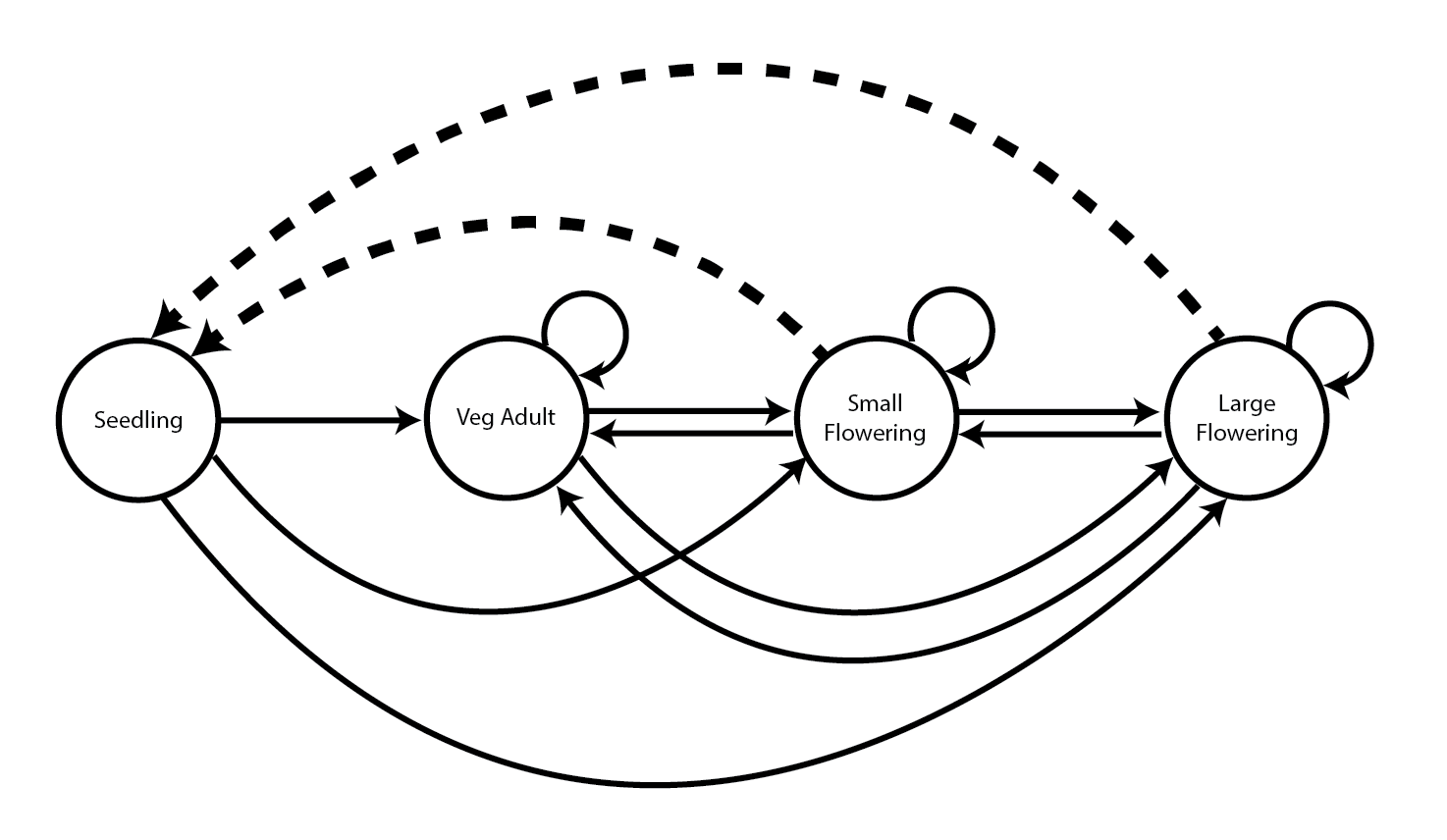
Next we will illustrate the one-way fixed LTRE, the stochastic LTRE, and the small noise approximation LTRE using the example published by Davison et al. (2010). That paper focused on nine natural populations of the perennial herb Anthyllis vulneraria, also known as kidney vetch, occurring in calcareous grasslands in the Viroin Valley of southwestern Belgium and monitored from 2003 to 2006. The published analysis included a stochastic LTRE. We provide a description of the plant and populations in section 1.8.3 of chapter 1. The plant is a short-lived, rosette-forming legume with a complex life cycle including stasis and retrogression between four stages but no seedbank (seedlings, juveniles, small adults and large adults; Figure 12.1).
12.4.1 Life history model development and data organization
We will first describe the life history characterizing the dataset, matching it to our analyses with a stageframe. Since we do not have the original demographic dataset that produced the published matrices, we do not need to know the exact sizes of plants and so will use proxy values. These proxy values must be unique and non-negative, and they need non-overlapping bins usable as size classes defining each stage. However, since we are not analyzing size itself here, they do not need any further basis in reality. Other characteristics must be exact and realistic to make sure that the analyses work properly, including all other stage descriptions such as reproductive status, propagule status, and observation status.
sizevector <- c(1, 1, 2, 3) # These sizes are not from the original paper
stagevector <- c("Sdl", "Veg", "SmFlo", "LFlo")
repvector <- c(0, 0, 1, 1)
obsvector <- c(1, 1, 1, 1)
matvector <- c(0, 1, 1, 1)
immvector <- c(1, 0, 0, 0)
propvector <- c(0, 0, 0, 0)
indataset <- c(1, 1, 1, 1)
binvec <- c(0.5, 0.5, 0.5, 0.5)
comments <- c("Seedling", "Vegetative adult", "Small flowering",
  "Large flowering")

anthframe <- sf_create(sizes = sizevector, stagenames = stagevector,
  repstatus = repvector, obsstatus = obsvector, matstatus = matvector,
  immstatus = immvector, indataset = indataset, binhalfwidth = binvec,
  propstatus = propvector, comments = comments)

anthframe
>   stage size size_b size_c min_age max_age repstatus obsstatus propstatus
> 1   Sdl    1     NA     NA      NA      NA         0         1          0
> 2   Veg    1     NA     NA      NA      NA         0         1          0
> 3 SmFlo    2     NA     NA      NA      NA         1         1          0
> 4  LFlo    3     NA     NA      NA      NA         1         1          0
>   immstatus matstatus indataset binhalfwidth_raw sizebin_min sizebin_max
> 1         1         0         1              0.5         0.5         1.5
> 2         0         1         1              0.5         0.5         1.5
> 3         0         1         1              0.5         1.5         2.5
> 4         0         1         1              0.5         2.5         3.5
>   sizebin_center sizebin_width binhalfwidthb_raw sizebinb_min sizebinb_max
> 1              1             1                NA           NA           NA
> 2              1             1                NA           NA           NA
> 3              2             1                NA           NA           NA
> 4              3             1                NA           NA           NA
>   sizebinb_center sizebinb_width binhalfwidthc_raw sizebinc_min sizebinc_max
> 1              NA             NA                NA           NA           NA
> 2              NA             NA                NA           NA           NA
> 3              NA             NA                NA           NA           NA
> 4              NA             NA                NA           NA           NA
>   sizebinc_center sizebinc_width group         comments
> 1              NA             NA     0         Seedling
> 2              NA             NA     0 Vegetative adult
> 3              NA             NA     0  Small flowering
> 4              NA             NA     0  Large flowering
Next, we will load data for this vignette, and then look at a summary.
data(anthyllis)
summary(anthyllis)
>
> This ahistorical lefkoMat object contains 27 matrices.
>
> Each matrix is square with 4 rows and columns, and a total of 16 elements.
> A total of 167 survival transitions were estimated, with 6.185 per matrix.
> A total of 48 fecundity transitions were estimated, with 1.778 per matrix.
> This lefkoMat object covers 1 population, 9 patches, and 3 time steps.
>
> This lefkoMat object appears to have been imported. Number of unique individuals and transitions not known.
>
> Survival probability sum check (each matrix represented by column in order):
>           [,1]  [,2]   [,3]   [,4]   [,5]  [,6]   [,7]  [,8]  [,9] [,10]  [,11]
> Min.    0.0667 0.500 0.0625 0.0769 0.0909 0.000 0.0000 0.333 0.171 0.000 0.0000
> 1st Qu. 0.0810 0.575 0.1708 0.1192 0.1334 0.075 0.0375 0.405 0.268 0.170 0.0000
> Median  0.1198 0.657 0.2106 0.3077 0.2276 0.100 0.1706 0.453 0.350 0.239 0.0000
> Mean    0.1599 0.637 0.2209 0.4231 0.2303 0.175 0.1895 0.469 0.320 0.203 0.0556
> 3rd Qu. 0.1987 0.720 0.2607 0.6116 0.3245 0.200 0.3225 0.517 0.402 0.271 0.0556
> Max.    0.3333 0.736 0.4000 1.0000 0.3750 0.500 0.4167 0.636 0.409 0.333 0.2222
>         [,12]  [,13] [,14]  [,15] [,16] [,17] [,18] [,19] [,20] [,21] [,22]
> Min.    0.000 0.0000 0.000 0.0370 0.333 0.000 0.238  0.00 0.000 0.000 0.000
> 1st Qu. 0.375 0.0000 0.193 0.0408 0.394 0.381 0.310  0.00 0.500 0.000 0.125
> Median  0.500 0.0163 0.313 0.0657 0.564 0.518 0.410  0.00 0.833 0.250 0.271
> Mean    0.409 0.0510 0.281 0.0705 0.565 0.420 0.388  0.25 0.667 0.304 0.260
> 3rd Qu. 0.534 0.0673 0.401 0.0954 0.736 0.557 0.488  0.25 1.000 0.554 0.406
> Max.    0.636 0.1714 0.500 0.1136 0.800 0.645 0.493  1.00 1.000 0.714 0.500
>         [,23] [,24]  [,25] [,26]  [,27]
> Min.    0.000 0.000 0.0000 0.000 0.0000
> 1st Qu. 0.500 0.250 0.0000 0.375 0.0833
> Median  0.762 0.333 0.0833 0.583 0.2556
> Mean    0.631 0.323 0.0833 0.542 0.3153
> 3rd Qu. 0.893 0.406 0.1667 0.750 0.4875
> Max.    1.000 0.625 0.1667 1.000 0.7500
>
>
> Stages without connections leading to the rest of the life cycle found in matrices: 5 7 10 11 12 13 19 20 21 23 24 25 26 27
We have 27 matrices, each four rows by four columns. These are raw matrices, so they are not completely full where matrix elements are possible. Let’s take a look at the first such matrix as an example.
anthyllis$A[[1]]
>            [,1]       [,2]       [,3]       [,4]
> [1,] 0.00000000 0.00000000 1.74000000 1.74000000
> [2,] 0.20833333 0.00000000 0.00000000 0.05714286
> [3,] 0.04166667 0.07692308 0.00000000 0.00000000
> [4,] 0.08333333 0.07692308 0.06666667 0.02857143
This is an \(\mathbf{A}\) matrix, meaning that it includes all survival-transitions and fecundity for population C as a whole over the interval 2003 to 2004. The corresponding \(\mathbf{U}\) and \(\mathbf{F}\) matrices were not provided in that paper, although it is most likely that the elements valued at 1.74 in the top right-hand corner are only composed of fecundity values while the rest of the matrix is only composed of survival transitions (this might not be the case if clonal reproduction were possible). The order of rows and columns corresponds to the order of stages in the stageframe anthframe.
Our anthyllis dataset is a full lefkoMat object, so it already includes a stage frame (in other words, we did not really need to make object anthframe). This is included as object ahstages within its structure. It also includes a labels element that shows the order of matrices by population, patch, and time. Let’s take a look at that object here.
anthyllis
> $A
> $A[[1]]
>            [,1]       [,2]       [,3]       [,4]
> [1,] 0.00000000 0.00000000 1.74000000 1.74000000
> [2,] 0.20833333 0.00000000 0.00000000 0.05714286
> [3,] 0.04166667 0.07692308 0.00000000 0.00000000
> [4,] 0.08333333 0.07692308 0.06666667 0.02857143
>
> $A[[2]]
>           [,1]      [,2] [,3] [,4]
> [1,] 0.0000000 0.0000000  0.3  0.6
> [2,] 0.3218391 0.1428571  0.0  0.0
> [3,] 0.1609195 0.2857143  0.0  0.0
> [4,] 0.2528736 0.2857143  0.5  0.6
>
> $A[[3]]
>      [,1]       [,2]    [,3]       [,4]
> [1,]  0.0 0.00000000 0.50625 0.67500000
> [2,]  0.0 0.00000000 0.00000 0.03571429
> [3,]  0.1 0.06896552 0.06250 0.10714286
> [4,]  0.3 0.13793103 0.00000 0.07142857
>
> $A[[4]]
>           [,1] [,2]      [,3]       [,4]
> [1,] 0.0000000  0.0 2.4400000 6.56923077
> [2,] 0.1964286  0.0 0.0000000 0.00000000
> [3,] 0.1250000  0.5 0.0000000 0.00000000
> [4,] 0.1607143  0.5 0.1333333 0.07692308
>
> $A[[5]]
>            [,1]       [,2]  [,3]       [,4]
> [1,] 0.00000000 0.00000000 0.450 0.64615385
> [2,] 0.06557377 0.09090909 0.125 0.00000000
> [3,] 0.03278689 0.00000000 0.125 0.07692308
> [4,] 0.04918033 0.00000000 0.125 0.23076923
>
> $A[[6]]
>            [,1] [,2] [,3] [,4]
> [1,] 0.00000000  0.0 2.85 3.99
> [2,] 0.08333333  0.0 0.00 0.00
> [3,] 0.00000000  0.0 0.00 0.00
> [4,] 0.41666667  0.1 0.00 0.10
>
> $A[[7]]
>            [,1] [,2]  [,3]       [,4]
> [1,] 0.00000000    0 1.815 7.05833333
> [2,] 0.07594937    0 0.050 0.08333333
> [3,] 0.13924051    0 0.000 0.25000000
> [4,] 0.07594937    0 0.000 0.08333333
>
> $A[[8]]
>           [,1]      [,2]       [,3]      [,4]
> [1,] 0.0000000 0.0000000 1.23333333 7.4000000
> [2,] 0.2238806 0.0000000 0.11111111 0.1428571
> [3,] 0.1343284 0.2727273 0.16666667 0.1428571
> [4,] 0.1194030 0.3636364 0.05555556 0.1428571
>
> $A[[9]]
>            [,1]  [,2]       [,3]      [,4]
> [1,] 0.00000000 0.000 1.06000000 3.3727273
> [2,] 0.07317073 0.025 0.03333333 0.0000000
> [3,] 0.03658537 0.150 0.10000000 0.1363636
> [4,] 0.06097561 0.225 0.16666667 0.2727273
>
> $A[[10]]
>       [,1] [,2]       [,3]      [,4]
> [1,] 0.000    0 0.24545454 2.1000000
> [2,] 0.000    0 0.04545454 0.0000000
> [3,] 0.125    0 0.09090909 0.0000000
> [4,] 0.125    0 0.09090909 0.3333333
>
> $A[[11]]
>           [,1] [,2] [,3] [,4]
> [1,] 0.0000000    0  1.1 1.54
> [2,] 0.1111111    0  0.0 0.00
> [3,] 0.0000000    0  0.0 0.00
> [4,] 0.1111111    0  0.0 0.00
>
> $A[[12]]
>            [,1] [,2] [,3] [,4]
> [1,] 0.00000000  0.0    0  1.5
> [2,] 0.00000000  0.0    0  0.0
> [3,] 0.09090909  0.0    0  0.0
> [4,] 0.54545455  0.5    0  0.5
>
> $A[[13]]
>            [,1] [,2]     [,3]       [,4]
> [1,] 0.00000000    0 1.785366 1.85652174
> [2,] 0.12857143    0 0.000000 0.01086956
> [3,] 0.02857143    0 0.000000 0.00000000
> [4,] 0.01428571    0 0.000000 0.02173913
>
> $A[[14]]
>           [,1]       [,2]  [,3]   [,4]
> [1,] 0.0000000 0.00000000 14.25 16.625
> [2,] 0.1314433 0.05714286  0.00  0.250
> [3,] 0.1443299 0.00000000  0.00  0.000
> [4,] 0.0927835 0.20000000  0.00  0.250
>
> $A[[15]]
>            [,1]       [,2]       [,3]       [,4]
> [1,] 0.00000000 0.00000000 0.59464286 1.76590909
> [2,] 0.00000000 0.00000000 0.01785714 0.00000000
> [3,] 0.02105263 0.01851852 0.03571429 0.04545454
> [4,] 0.02105263 0.01851852 0.03571429 0.06818182
>
> $A[[16]]
>      [,1]      [,2]       [,3]      [,4]
> [1,] 0.00 0.0000000 11.5000000 2.7758621
> [2,] 0.60 0.2857143  0.3333333 0.2413793
> [3,] 0.04 0.1428571  0.0000000 0.0000000
> [4,] 0.16 0.2857143  0.0000000 0.1724138
>
> $A[[17]]
>            [,1]       [,2] [,3]       [,4]
> [1,] 0.00000000 0.00000000 3.78 1.22500000
> [2,] 0.28358209 0.17105263 0.00 0.16666667
> [3,] 0.08457711 0.02631579 0.00 0.05555556
> [4,] 0.13930348 0.44736842 0.00 0.30555556
>
> $A[[18]]
>           [,1]      [,2]       [,3]       [,4]
> [1,] 0.0000000 0.0000000 1.54285714 1.03561644
> [2,] 0.1269841 0.1052632 0.04761905 0.05479452
> [3,] 0.0952381 0.1578947 0.19047619 0.08219178
> [4,] 0.1111111 0.2236842 0.00000000 0.35616438
>
> $A[[19]]
>      [,1] [,2] [,3]  [,4]
> [1,]    0    0 0.15 0.175
> [2,]    0    0 0.00 0.000
> [3,]    0    0 0.00 0.000
> [4,]    1    0 0.00 0.000
>
> $A[[20]]
>      [,1]      [,2] [,3] [,4]
> [1,]    0 0.0000000    0 0.25
> [2,]    0 0.0000000    0 0.00
> [3,]    0 0.0000000    0 0.00
> [4,]    1 0.6666667    0 1.00
>
> $A[[21]]
>      [,1] [,2] [,3]      [,4]
> [1,] 0.00    0    0 1.4285714
> [2,] 0.00    0    0 0.1428571
> [3,] 0.25    0    0 0.0000000
> [4,] 0.25    0    0 0.5714286
>
> $A[[22]]
>      [,1]      [,2] [,3]   [,4]
> [1,] 0.00 0.0000000  0.7 0.6125
> [2,] 0.25 0.0000000  0.0 0.1250
> [3,] 0.00 0.0000000  0.0 0.0000
> [4,] 0.25 0.1666667  0.0 0.2500
>
> $A[[23]]
>           [,1]      [,2] [,3] [,4]
> [1,] 0.0000000 0.0000000    0  0.6
> [2,] 0.2857143 0.0000000    0  0.0
> [3,] 0.2857143 0.3333333    0  0.0
> [4,] 0.2857143 0.3333333    0  1.0
>
> $A[[24]]
>           [,1] [,2]      [,3]   [,4]
> [1,] 0.0000000    0 0.7000000 0.6125
> [2,] 0.0000000    0 0.0000000 0.0000
> [3,] 0.0000000    0 0.0000000 0.0000
> [4,] 0.3333333    0 0.3333333 0.6250
>
> $A[[25]]
>           [,1] [,2] [,3]      [,4]
> [1,] 0.0000000    0  2.1 0.8166667
> [2,] 0.1666667    0  0.0 0.0000000
> [3,] 0.0000000    0  0.0 0.0000000
> [4,] 0.0000000    0  0.0 0.1666667
>
> $A[[26]]
>           [,1] [,2] [,3] [,4]
> [1,] 0.0000000  0.0    0    7
> [2,] 0.3333333  0.5    0    0
> [3,] 0.0000000  0.0    0    0
> [4,] 0.3333333  0.0    0    1
>
> $A[[27]]
>           [,1] [,2] [,3] [,4]
> [1,] 0.0000000 0.00    0  1.4
> [2,] 0.0000000 0.00    0  0.0
> [3,] 0.0000000 0.00    0  0.2
> [4,] 0.1111111 0.75    0  0.2
>
>
> $U
> $U[[1]]
>            [,1]       [,2]       [,3]       [,4]
> [1,] 0.00000000 0.00000000 0.00000000 0.00000000
> [2,] 0.20833333 0.00000000 0.00000000 0.05714286
> [3,] 0.04166667 0.07692308 0.00000000 0.00000000
> [4,] 0.08333333 0.07692308 0.06666667 0.02857143
>
> $U[[2]]
>           [,1]      [,2] [,3] [,4]
> [1,] 0.0000000 0.0000000  0.0  0.0
> [2,] 0.3218391 0.1428571  0.0  0.0
> [3,] 0.1609195 0.2857143  0.0  0.0
> [4,] 0.2528736 0.2857143  0.5  0.6
>
> $U[[3]]
>      [,1]       [,2]   [,3]       [,4]
> [1,]  0.0 0.00000000 0.0000 0.00000000
> [2,]  0.0 0.00000000 0.0000 0.03571429
> [3,]  0.1 0.06896552 0.0625 0.10714286
> [4,]  0.3 0.13793103 0.0000 0.07142857
>
> $U[[4]]
>           [,1] [,2]      [,3]       [,4]
> [1,] 0.0000000  0.0 0.0000000 0.00000000
> [2,] 0.1964286  0.0 0.0000000 0.00000000
> [3,] 0.1250000  0.5 0.0000000 0.00000000
> [4,] 0.1607143  0.5 0.1333333 0.07692308
>
> $U[[5]]
>            [,1]       [,2]  [,3]       [,4]
> [1,] 0.00000000 0.00000000 0.000 0.00000000
> [2,] 0.06557377 0.09090909 0.125 0.00000000
> [3,] 0.03278689 0.00000000 0.125 0.07692308
> [4,] 0.04918033 0.00000000 0.125 0.23076923
>
> $U[[6]]
>            [,1] [,2] [,3] [,4]
> [1,] 0.00000000  0.0    0  0.0
> [2,] 0.08333333  0.0    0  0.0
> [3,] 0.00000000  0.0    0  0.0
> [4,] 0.41666667  0.1    0  0.1
>
> $U[[7]]
>            [,1] [,2] [,3]       [,4]
> [1,] 0.00000000    0 0.00 0.00000000
> [2,] 0.07594937    0 0.05 0.08333333
> [3,] 0.13924051    0 0.00 0.25000000
> [4,] 0.07594937    0 0.00 0.08333333
>
> $U[[8]]
>           [,1]      [,2]       [,3]      [,4]
> [1,] 0.0000000 0.0000000 0.00000000 0.0000000
> [2,] 0.2238806 0.0000000 0.11111111 0.1428571
> [3,] 0.1343284 0.2727273 0.16666667 0.1428571
> [4,] 0.1194030 0.3636364 0.05555556 0.1428571
>
> $U[[9]]
>            [,1]  [,2]       [,3]      [,4]
> [1,] 0.00000000 0.000 0.00000000 0.0000000
> [2,] 0.07317073 0.025 0.03333333 0.0000000
> [3,] 0.03658537 0.150 0.10000000 0.1363636
> [4,] 0.06097561 0.225 0.16666667 0.2727273
>
> $U[[10]]
>       [,1] [,2]       [,3]      [,4]
> [1,] 0.000    0 0.00000000 0.0000000
> [2,] 0.000    0 0.04545454 0.0000000
> [3,] 0.125    0 0.09090909 0.0000000
> [4,] 0.125    0 0.09090909 0.3333333
>
> $U[[11]]
>           [,1] [,2] [,3] [,4]
> [1,] 0.0000000    0    0    0
> [2,] 0.1111111    0    0    0
> [3,] 0.0000000    0    0    0
> [4,] 0.1111111    0    0    0
>
> $U[[12]]
>            [,1] [,2] [,3] [,4]
> [1,] 0.00000000  0.0    0  0.0
> [2,] 0.00000000  0.0    0  0.0
> [3,] 0.09090909  0.0    0  0.0
> [4,] 0.54545455  0.5    0  0.5
>
> $U[[13]]
>            [,1] [,2] [,3]       [,4]
> [1,] 0.00000000    0    0 0.00000000
> [2,] 0.12857143    0    0 0.01086956
> [3,] 0.02857143    0    0 0.00000000
> [4,] 0.01428571    0    0 0.02173913
>
> $U[[14]]
>           [,1]       [,2] [,3] [,4]
> [1,] 0.0000000 0.00000000    0 0.00
> [2,] 0.1314433 0.05714286    0 0.25
> [3,] 0.1443299 0.00000000    0 0.00
> [4,] 0.0927835 0.20000000    0 0.25
>
> $U[[15]]
>            [,1]       [,2]       [,3]       [,4]
> [1,] 0.00000000 0.00000000 0.00000000 0.00000000
> [2,] 0.00000000 0.00000000 0.01785714 0.00000000
> [3,] 0.02105263 0.01851852 0.03571429 0.04545454
> [4,] 0.02105263 0.01851852 0.03571429 0.06818182
>
> $U[[16]]
>      [,1]      [,2]      [,3]      [,4]
> [1,] 0.00 0.0000000 0.0000000 0.0000000
> [2,] 0.60 0.2857143 0.3333333 0.2413793
> [3,] 0.04 0.1428571 0.0000000 0.0000000
> [4,] 0.16 0.2857143 0.0000000 0.1724138
>
> $U[[17]]
>            [,1]       [,2] [,3]       [,4]
> [1,] 0.00000000 0.00000000    0 0.00000000
> [2,] 0.28358209 0.17105263    0 0.16666667
> [3,] 0.08457711 0.02631579    0 0.05555556
> [4,] 0.13930348 0.44736842    0 0.30555556
>
> $U[[18]]
>           [,1]      [,2]       [,3]       [,4]
> [1,] 0.0000000 0.0000000 0.00000000 0.00000000
> [2,] 0.1269841 0.1052632 0.04761905 0.05479452
> [3,] 0.0952381 0.1578947 0.19047619 0.08219178
> [4,] 0.1111111 0.2236842 0.00000000 0.35616438
>
> $U[[19]]
>      [,1] [,2] [,3] [,4]
> [1,]    0    0    0    0
> [2,]    0    0    0    0
> [3,]    0    0    0    0
> [4,]    1    0    0    0
>
> $U[[20]]
>      [,1]      [,2] [,3] [,4]
> [1,]    0 0.0000000    0    0
> [2,]    0 0.0000000    0    0
> [3,]    0 0.0000000    0    0
> [4,]    1 0.6666667    0    1
>
> $U[[21]]
>      [,1] [,2] [,3]      [,4]
> [1,] 0.00    0    0 0.0000000
> [2,] 0.00    0    0 0.1428571
> [3,] 0.25    0    0 0.0000000
> [4,] 0.25    0    0 0.5714286
>
> $U[[22]]
>      [,1]      [,2] [,3]  [,4]
> [1,] 0.00 0.0000000    0 0.000
> [2,] 0.25 0.0000000    0 0.125
> [3,] 0.00 0.0000000    0 0.000
> [4,] 0.25 0.1666667    0 0.250
>
> $U[[23]]
>           [,1]      [,2] [,3] [,4]
> [1,] 0.0000000 0.0000000    0    0
> [2,] 0.2857143 0.0000000    0    0
> [3,] 0.2857143 0.3333333    0    0
> [4,] 0.2857143 0.3333333    0    1
>
> $U[[24]]
>           [,1] [,2]      [,3]  [,4]
> [1,] 0.0000000    0 0.0000000 0.000
> [2,] 0.0000000    0 0.0000000 0.000
> [3,] 0.0000000    0 0.0000000 0.000
> [4,] 0.3333333    0 0.3333333 0.625
>
> $U[[25]]
>           [,1] [,2] [,3]      [,4]
> [1,] 0.0000000    0    0 0.0000000
> [2,] 0.1666667    0    0 0.0000000
> [3,] 0.0000000    0    0 0.0000000
> [4,] 0.0000000    0    0 0.1666667
>
> $U[[26]]
>           [,1] [,2] [,3] [,4]
> [1,] 0.0000000  0.0    0    0
> [2,] 0.3333333  0.5    0    0
> [3,] 0.0000000  0.0    0    0
> [4,] 0.3333333  0.0    0    1
>
> $U[[27]]
>           [,1] [,2] [,3] [,4]
> [1,] 0.0000000 0.00    0  0.0
> [2,] 0.0000000 0.00    0  0.0
> [3,] 0.0000000 0.00    0  0.2
> [4,] 0.1111111 0.75    0  0.2
>
>
> $F
> $F[[1]]
>      [,1] [,2] [,3] [,4]
> [1,]    0    0 1.74 1.74
> [2,]    0    0 0.00 0.00
> [3,]    0    0 0.00 0.00
> [4,]    0    0 0.00 0.00
>
> $F[[2]]
>      [,1] [,2] [,3] [,4]
> [1,]    0    0  0.3  0.6
> [2,]    0    0  0.0  0.0
> [3,]    0    0  0.0  0.0
> [4,]    0    0  0.0  0.0
>
> $F[[3]]
>      [,1] [,2]    [,3]  [,4]
> [1,]    0    0 0.50625 0.675
> [2,]    0    0 0.00000 0.000
> [3,]    0    0 0.00000 0.000
> [4,]    0    0 0.00000 0.000
>
> $F[[4]]
>      [,1] [,2] [,3]     [,4]
> [1,]    0    0 2.44 6.569231
> [2,]    0    0 0.00 0.000000
> [3,]    0    0 0.00 0.000000
> [4,]    0    0 0.00 0.000000
>
> $F[[5]]
>      [,1] [,2] [,3]      [,4]
> [1,]    0    0 0.45 0.6461538
> [2,]    0    0 0.00 0.0000000
> [3,]    0    0 0.00 0.0000000
> [4,]    0    0 0.00 0.0000000
>
> $F[[6]]
>      [,1] [,2] [,3] [,4]
> [1,]    0    0 2.85 3.99
> [2,]    0    0 0.00 0.00
> [3,]    0    0 0.00 0.00
> [4,]    0    0 0.00 0.00
>
> $F[[7]]
>      [,1] [,2]  [,3]     [,4]
> [1,]    0    0 1.815 7.058333
> [2,]    0    0 0.000 0.000000
> [3,]    0    0 0.000 0.000000
> [4,]    0    0 0.000 0.000000
>
> $F[[8]]
>      [,1] [,2]     [,3] [,4]
> [1,]    0    0 1.233333  7.4
> [2,]    0    0 0.000000  0.0
> [3,]    0    0 0.000000  0.0
> [4,]    0    0 0.000000  0.0
>
> $F[[9]]
>      [,1] [,2] [,3]     [,4]
> [1,]    0    0 1.06 3.372727
> [2,]    0    0 0.00 0.000000
> [3,]    0    0 0.00 0.000000
> [4,]    0    0 0.00 0.000000
>
> $F[[10]]
>      [,1] [,2]      [,3] [,4]
> [1,]    0    0 0.2454545  2.1
> [2,]    0    0 0.0000000  0.0
> [3,]    0    0 0.0000000  0.0
> [4,]    0    0 0.0000000  0.0
>
> $F[[11]]
>      [,1] [,2] [,3] [,4]
> [1,]    0    0  1.1 1.54
> [2,]    0    0  0.0 0.00
> [3,]    0    0  0.0 0.00
> [4,]    0    0  0.0 0.00
>
> $F[[12]]
>      [,1] [,2] [,3] [,4]
> [1,]    0    0    0  1.5
> [2,]    0    0    0  0.0
> [3,]    0    0    0  0.0
> [4,]    0    0    0  0.0
>
> $F[[13]]
>      [,1] [,2]     [,3]     [,4]
> [1,]    0    0 1.785366 1.856522
> [2,]    0    0 0.000000 0.000000
> [3,]    0    0 0.000000 0.000000
> [4,]    0    0 0.000000 0.000000
>
> $F[[14]]
>      [,1] [,2]  [,3]   [,4]
> [1,]    0    0 14.25 16.625
> [2,]    0    0  0.00  0.000
> [3,]    0    0  0.00  0.000
> [4,]    0    0  0.00  0.000
>
> $F[[15]]
>      [,1] [,2]      [,3]     [,4]
> [1,]    0    0 0.5946429 1.765909
> [2,]    0    0 0.0000000 0.000000
> [3,]    0    0 0.0000000 0.000000
> [4,]    0    0 0.0000000 0.000000
>
> $F[[16]]
>      [,1] [,2] [,3]     [,4]
> [1,]    0    0 11.5 2.775862
> [2,]    0    0  0.0 0.000000
> [3,]    0    0  0.0 0.000000
> [4,]    0    0  0.0 0.000000
>
> $F[[17]]
>      [,1] [,2] [,3]  [,4]
> [1,]    0    0 3.78 1.225
> [2,]    0    0 0.00 0.000
> [3,]    0    0 0.00 0.000
> [4,]    0    0 0.00 0.000
>
> $F[[18]]
>      [,1] [,2]     [,3]     [,4]
> [1,]    0    0 1.542857 1.035616
> [2,]    0    0 0.000000 0.000000
> [3,]    0    0 0.000000 0.000000
> [4,]    0    0 0.000000 0.000000
>
> $F[[19]]
>      [,1] [,2] [,3]  [,4]
> [1,]    0    0 0.15 0.175
> [2,]    0    0 0.00 0.000
> [3,]    0    0 0.00 0.000
> [4,]    0    0 0.00 0.000
>
> $F[[20]]
>      [,1] [,2] [,3] [,4]
> [1,]    0    0    0 0.25
> [2,]    0    0    0 0.00
> [3,]    0    0    0 0.00
> [4,]    0    0    0 0.00
>
> $F[[21]]
>      [,1] [,2] [,3]     [,4]
> [1,]    0    0    0 1.428571
> [2,]    0    0    0 0.000000
> [3,]    0    0    0 0.000000
> [4,]    0    0    0 0.000000
>
> $F[[22]]
>      [,1] [,2] [,3]   [,4]
> [1,]    0    0  0.7 0.6125
> [2,]    0    0  0.0 0.0000
> [3,]    0    0  0.0 0.0000
> [4,]    0    0  0.0 0.0000
>
> $F[[23]]
>      [,1] [,2] [,3] [,4]
> [1,]    0    0    0  0.6
> [2,]    0    0    0  0.0
> [3,]    0    0    0  0.0
> [4,]    0    0    0  0.0
>
> $F[[24]]
>      [,1] [,2] [,3]   [,4]
> [1,]    0    0  0.7 0.6125
> [2,]    0    0  0.0 0.0000
> [3,]    0    0  0.0 0.0000
> [4,]    0    0  0.0 0.0000
>
> $F[[25]]
>      [,1] [,2] [,3]      [,4]
> [1,]    0    0  2.1 0.8166667
> [2,]    0    0  0.0 0.0000000
> [3,]    0    0  0.0 0.0000000
> [4,]    0    0  0.0 0.0000000
>
> $F[[26]]
>      [,1] [,2] [,3] [,4]
> [1,]    0    0    0    7
> [2,]    0    0    0    0
> [3,]    0    0    0    0
> [4,]    0    0    0    0
>
> $F[[27]]
>      [,1] [,2] [,3] [,4]
> [1,]    0    0    0  1.4
> [2,]    0    0    0  0.0
> [3,]    0    0    0  0.0
> [4,]    0    0    0  0.0
>
>
> $hstages
> [1] NA
>
> $agestages
> [1] NA
>
> $ahstages
>   stage_id stage_id stage original_size original_size_b original_size_c min_age
> 1        1        1   Sdl             1              NA              NA       0
> 2        2        2   Veg             1              NA              NA       0
> 3        3        3 SmFlo             2              NA              NA       0
> 4        4        4  LFlo             3              NA              NA       0
>   max_age repstatus obsstatus propstatus immstatus matstatus entrystage
> 1      NA         0         1          0         1         0          1
> 2      NA         0         1          0         0         1          0
> 3      NA         1         1          0         0         1          0
> 4      NA         1         1          0         0         1          0
>   indataset binhalfwidth_raw sizebin_min sizebin_max sizebin_center
> 1         1              0.5         0.5         1.5              1
> 2         1              0.5         0.5         1.5              1
> 3         1              0.5         1.5         2.5              2
> 4         1              0.5         2.5         3.5              3
>   sizebin_width binhalfwidthb_raw sizebinb_min sizebinb_max sizebinb_center
> 1             1                NA           NA           NA              NA
> 2             1                NA           NA           NA              NA
> 3             1                NA           NA           NA              NA
> 4             1                NA           NA           NA              NA
>   sizebinb_width binhalfwidthc_raw sizebinc_min sizebinc_max sizebinc_center
> 1             NA                NA           NA           NA              NA
> 2             NA                NA           NA           NA              NA
> 3             NA                NA           NA           NA              NA
> 4             NA                NA           NA           NA              NA
>   sizebinc_width group         comments alive almostborn
> 1             NA     0         Seedling     1          0
> 2             NA     0 Vegetative adult     1          0
> 3             NA     0  Small flowering     1          0
> 4             NA     0  Large flowering     1          0
>
> $labels
>    pop patch year2
> 1    1     C  2003
> 2    1     C  2004
> 3    1     C  2005
> 4    1     E  2003
> 5    1     E  2004
> 6    1     E  2005
> 7    1     F  2003
> 8    1     F  2004
> 9    1     F  2005
> 10   1     G  2003
> 11   1     G  2004
> 12   1     G  2005
> 13   1     L  2003
> 14   1     L  2004
> 15   1     L  2005
> 16   1     O  2003
> 17   1     O  2004
> 18   1     O  2005
> 19   1     Q  2003
> 20   1     Q  2004
> 21   1     Q  2005
> 22   1     R  2003
> 23   1     R  2004
> 24   1     R  2005
> 25   1     S  2003
> 26   1     S  2004
> 27   1     S  2005
>
> $matrixqc
> [1] 167  48  27
>
> $dataqc
> [1] NA NA
>
> attr(,"class")
> [1] "lefkoMat"
The resulting object has all of the elements of a standard lefkoMat object except for those elements related to quality control in the demographic dataset and linear modeling. The option UFdecomp was left at its default (UFdecomp = TRUE), and so create_lM() used the stageframe to infer where fecundity values were located in the matrices and created \(\mathbf{U}\) and \(\mathbf{F}\) matrices separating those values. The default option for historical is set to FALSE, yielding an NA in place of the hstages element, which would typically list the order of historical stage pairs.
12.4.2 LTRE analysis
Now, we will develop arithmetic mean matrices and assess the deterministic and stochastic population growth rates, \(\lambda\) and \(a\), respectively (figure 12.2).
anth_lmean <- lmean(anthyllis)

lambda2 <- lambda3(anthyllis)
lambda2m <- lambda3(anth_lmean)

set.seed(42)
sl2 <- slambda3(anthyllis) #Stochastic growth rate
sl2$expa <- exp(sl2$a)

plot(lambda ~ as.integer(year2), data = lambda2,
  ylim = c(0, 2.5), xlim = c(2003, 2005), xlab = "Year",
  ylab = expression(lambda), type = "l", col = "gray", lty= 2, lwd = 2,
  bty = "n")
lines(lambda ~ year2, data = subset(lambda2, patch == 2), col = "gray", lty= 2,
  lwd = 2)
lines(lambda ~ year2, data = subset(lambda2, patch == 3), col = "gray", lty= 2,
  lwd = 2)
lines(lambda ~ year2, data = subset(lambda2, patch == 4), col = "gray", lty= 2,
  lwd = 2)
lines(lambda ~ year2, data = subset(lambda2, patch == 5), col = "gray", lty= 2,
  lwd = 2)
lines(lambda ~ year2, data = subset(lambda2, patch == 6), col = "gray", lty= 2,
  lwd = 2)
lines(lambda ~ year2, data = subset(lambda2, patch == 7), col = "gray", lty= 2,
  lwd = 2)
lines(lambda ~ year2, data = subset(lambda2, patch == 8), col = "gray", lty= 2,
  lwd = 2)
lines(lambda ~ year2, data = subset(lambda2, patch == 9), col = "gray", lty= 2,
  lwd = 2)
abline(a = lambda2m$lambda[1], b = 0, lty = 1, lwd = 4, col = "orangered")
abline(a = sl2$expa[1], b = 0, lty = 1, lwd = 4, col = "darkred")
legend("topleft", c("det annual", "det mean", "stochastic"), lty = c(2, 1, 1),
  col = c("gray", "orangered", "darkred"), lwd = c(2, 4, 4), bty = "n")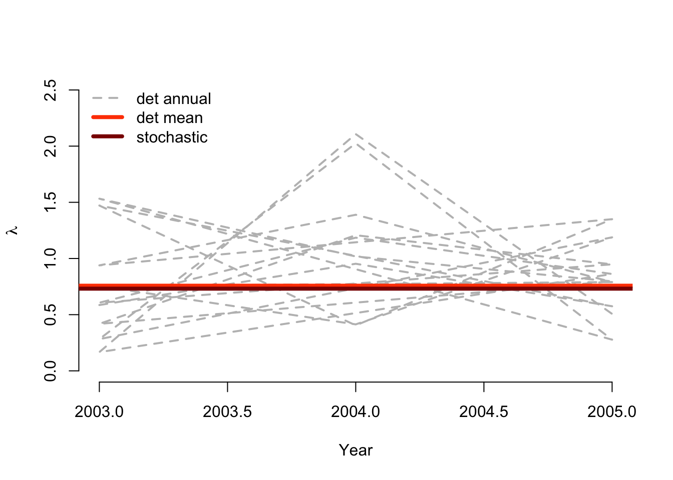
Figure 12.2: Deterministic vs. stochastic lambda of Anthyllis populations
Clearly, these populations exhibit extremely variable growth across the short field study during which they were monitored. Also very clear is that these populations appear to be on the decline, as shown by \(\lambda\) for the overall mean matrix, and \(e\) to the power of the stochastic growth rate \(a = \text{log} \lambda\).
12.4.2.1 Deterministic LTREs
Let’s conduct a one-way, fixed life table response experiment (LTRE) next. This will be a deterministic LTRE against the input matrices, meaning that we will assess the impacts of differences in matrix elements between the core matrices input and the overall arithmetic grand mean matrix on differences in the deterministic growth rate, \(\lambda\). Since it is not appropriate to assess the differences due to time this way, we will conduct this LTRE using the patch-level mean matrices from anth_lmean against the grand mean. In other words, we will use this one-way fixed LTRE to test the impact of patch on the asymptotic growth rate.
Let’s take a look at the labels element to this object first. Note in the output below that we have 10 matrices, including nine population matrices and one overall among-population mean.
anth_lmean$labels
>    pop patch
> 1    1     C
> 2    1     E
> 3    1     F
> 4    1     G
> 5    1     L
> 6    1     O
> 7    1     Q
> 8    1     R
> 9    1     S
> 10   1     0
One key problem is that the grand mean is actually included as the last matrix. We do not wish to run an LTRE in which the reference matrix is also a treatment matrix, so we will first delete the grand mean from this object, and use the resulting lefkoMat object in our LTRE. Let’s delete the final matrix as below.
pruned_anth_lmean <- delete_lM(anth_lmean, mat_num = 10)
pruned_anth_lmean$labels
>   pop patch
> 1   1     C
> 2   1     E
> 3   1     F
> 4   1     G
> 5   1     L
> 6   1     O
> 7   1     Q
> 8   1     R
> 9   1     S
Success! Now, let’s run the ltre3() function. We will use the default settings, which set the reference as the grand mean matrix (this is computed automatically during the LTRE run). We could use a different reference matrix if we wished, and this would be specified by setting the refmats option to an appropriate reference lefkoMat object.
trialltre_det <- ltre3(pruned_anth_lmean)
> Warning: Matrices input as mats will also be used in reference matrix
> calculation.
> Using all refmats matrices in reference matrix calculation.
trialltre_det
> $cont_mean
> $cont_mean[[1]]
>             [,1]          [,2]          [,3]         [,4]
> [1,]  0.00000000  0.0000000000 -0.0526643830 -0.278604545
> [2,]  0.01288781 -0.0002075509 -0.0011802734 -0.002247916
> [3,]  0.02099388  0.0095296944 -0.0007380232 -0.001431440
> [4,] -0.02838087 -0.0062826320  0.0199742696 -0.036219658
>
> $cont_mean[[2]]
>              [,1]          [,2]         [,3]         [,4]
> [1,]  0.000000000  0.0000000000 0.0010320913  0.113969244
> [2,] -0.008180535 -0.0010477967 0.0004334319 -0.005568240
> [3,] -0.016462320  0.0100496346 0.0009236077 -0.003737373
> [4,] -0.045108893  0.0008961807 0.0039524441 -0.081432730
>
> $cont_mean[[3]]
>              [,1]          [,2]         [,3]         [,4]
> [1,]  0.000000000  0.0000000000 -0.024063752  0.275500504
> [2,] -0.005037786 -0.0025268625  0.001872599  0.002568217
> [3,]  0.023776228  0.0066160079  0.005270105  0.022131728
> [4,] -0.315031272  0.0001712855  0.004413070 -0.065764758
>
> $cont_mean[[4]]
>               [,1]         [,2]          [,3]         [,4]
> [1,]  0.0000000000  0.000000000 -5.028329e-02 -0.169540748
> [2,] -0.0269687794 -0.001420158 -3.137497e-04 -0.005202208
> [3,]  0.0001492085 -0.004256203  8.430731e-05 -0.008839788
> [4,]  0.0311640114 -0.003928060 -2.974225e-03 -0.017954340
>
> $cont_mean[[5]]
>             [,1]        [,2]         [,3]         [,4]
> [1,]  0.00000000  0.00000000  0.112678253  0.300395132
> [2,] -0.01743882 -0.00131768 -0.000567669  0.002407567
> [3,] -0.01091381 -0.01241459 -0.001846088 -0.006955586
> [4,] -0.46041272 -0.03371817 -0.007443071 -0.083077750
>
> $cont_mean[[6]]
>              [,1]       [,2]         [,3]         [,4]
> [1,]  0.000000000 0.00000000  0.145611873 -0.132570128
> [2,]  0.085120191 0.01611388  0.004397356  0.014357161
> [3,]  0.002147524 0.01287140  0.005025013  0.002326089
> [4,] -0.114627718 0.03934714 -0.006712288 -0.012485180
>
> $cont_mean[[7]]
>              [,1]          [,2]          [,3]          [,4]
> [1,]  0.000000000  0.0000000000 -0.0565636772 -0.5554555750
> [2,] -0.022442169 -0.0007237743 -0.0003715165 -0.0001003139
> [3,]  0.003947167 -0.0021924335 -0.0007702247 -0.0090681614
> [4,]  0.444644607  0.0019804891 -0.0038457456  0.1207791604
>
> $cont_mean[[8]]
>             [,1]         [,2]          [,3]          [,4]
> [1,] 0.000000000  0.000000000 -0.0524795118 -0.3990970676
> [2,] 0.009959864 -0.002144705 -0.0007147407 -0.0008570809
> [3,] 0.011313284  0.003107712 -0.0014907816 -0.0104568792
> [4,] 0.055374257 -0.005505580  0.0063263888  0.1766385565
>
> $cont_mean[[9]]
>             [,1]         [,2]          [,3]         [,4]
> [1,]  0.00000000  0.000000000 -0.0245397016  0.034433102
> [2,]  0.01213148  0.007593275 -0.0006363292 -0.006457662
> [3,] -0.03527604 -0.006195371 -0.0008050954  0.004342704
> [4,] -0.14291846  0.014609995 -0.0051357739  0.078041234
>
>
> $ahstages
>   stage_id stage_id stage original_size original_size_b original_size_c min_age
> 1        1        1   Sdl             1              NA              NA       0
> 2        2        2   Veg             1              NA              NA       0
> 3        3        3 SmFlo             2              NA              NA       0
> 4        4        4  LFlo             3              NA              NA       0
>   max_age repstatus obsstatus propstatus immstatus matstatus entrystage
> 1      NA         0         1          0         1         0          1
> 2      NA         0         1          0         0         1          0
> 3      NA         1         1          0         0         1          0
> 4      NA         1         1          0         0         1          0
>   indataset binhalfwidth_raw sizebin_min sizebin_max sizebin_center
> 1         1              0.5         0.5         1.5              1
> 2         1              0.5         0.5         1.5              1
> 3         1              0.5         1.5         2.5              2
> 4         1              0.5         2.5         3.5              3
>   sizebin_width binhalfwidthb_raw sizebinb_min sizebinb_max sizebinb_center
> 1             1                NA           NA           NA              NA
> 2             1                NA           NA           NA              NA
> 3             1                NA           NA           NA              NA
> 4             1                NA           NA           NA              NA
>   sizebinb_width binhalfwidthc_raw sizebinc_min sizebinc_max sizebinc_center
> 1             NA                NA           NA           NA              NA
> 2             NA                NA           NA           NA              NA
> 3             NA                NA           NA           NA              NA
> 4             NA                NA           NA           NA              NA
>   sizebinc_width group         comments alive almostborn
> 1             NA     0         Seedling     1          0
> 2             NA     0 Vegetative adult     1          0
> 3             NA     0  Small flowering     1          0
> 4             NA     0  Large flowering     1          0
>
> $agestages
>   NA
> 1 NA
>
> $hstages
>   NA
> 1 NA
>
> $labels
>   pop patch
> 1   1     C
> 2   1     E
> 3   1     F
> 4   1     G
> 5   1     L
> 6   1     O
> 7   1     Q
> 8   1     R
> 9   1     S
>
> attr(,"class")
> [1] "lefkoLTRE"
The resulting lefkoLTRE object gives the LTRE contributions for each patch-level mean matrix relative to the arithmetic grand mean matrix. These are provided within the top list, cont_mean. These differences in LTRE contributions are essentially across space, and so are of interest if we wished to analyze these patterns geographically. They do not provide us with any understanding of how time affects population dynamics, though (we tackle this issue in section 12.4.2.4). Let’s move on to a method that will help us assess differences between the treatment group of matrices and the reference while accounting for time.
12.4.2.2 Stochastic LTREs (sLTRE)
To assess the contributions across space while accounting for temporal shifts, we should conduct either a stochastic LTRE (sLTRE) or a small noise approximation LTRE (SNA-LTRE) on the original lefkoMat object holding the annual matrices. Let’s conduct a stochastic LTRE first, as below.
set.seed(42)

trialltre_sto <- ltre3(anthyllis, stochastic = TRUE, times = 10000)
> Warning: Matrices input as mats will also be used in reference matrix
> calculation.
> Using all refmats matrices in reference matrix calculation.
trialltre_sto
> $cont_mean
> $cont_mean[[1]]
>             [,1]          [,2]          [,3]         [,4]
> [1,]  0.00000000  0.0000000000 -0.0513533051 -0.370046268
> [2,]  0.01070441 -0.0001494254  0.0027369205 -0.002247365
> [3,]  0.01788772  0.0050314355 -0.0005986834 -0.001314109
> [4,] -0.03532046 -0.0058505178  0.0082361463 -0.041674065
>
> $cont_mean[[2]]
>             [,1]          [,2]         [,3]         [,4]
> [1,]  0.00000000  0.0000000000 0.0010274104  0.105480532
> [2,] -0.00670430 -0.0011243580 0.0002973440  0.015110168
> [3,] -0.01624259  0.0061747842 0.0007160183 -0.004703255
> [4,] -0.04015015  0.0008191957 0.0029287984 -0.119114673
>
> $cont_mean[[3]]
>              [,1]          [,2]         [,3]         [,4]
> [1,]  0.000000000  0.0000000000 -0.020524621  0.273751165
> [2,] -0.003574792 -0.0039090129  0.000636509  0.002199345
> [3,]  0.019182616  0.0048699336  0.002153131  0.015022612
> [4,] -0.322709908  0.0001153208  0.001911457 -0.090186808
>
> $cont_mean[[4]]
>               [,1]         [,2]          [,3]        [,4]
> [1,]  0.0000000000  0.000000000 -0.0924600728 -0.17681626
> [2,] -0.0527549465  0.006417614 -0.0004791935  0.01511017
> [3,]  0.0001962598  0.020101197  0.0001120028  0.03276793
> [4,]  0.0297327493 -0.005892341 -0.0041275991 -0.01669656
>
> $cont_mean[[5]]
>              [,1]         [,2]         [,3]         [,4]
> [1,]  0.000000000  0.000000000  0.069577353  0.319784869
> [2,] -0.018228417 -0.002125866 -0.001196399  0.002911781
> [3,] -0.005424845 -0.019442038 -0.001660114 -0.010084176
> [4,] -0.541943334 -0.036362625 -0.010440234 -0.145158921
>
> $cont_mean[[6]]
>              [,1]        [,2]        [,3]         [,4]
> [1,]  0.000000000 0.000000000 0.070320347 -0.184186064
> [2,]  0.036900148 0.002805042 0.001152763  0.005775457
> [3,]  0.001136099 0.002875825 0.001514940  0.001255778
> [4,] -0.173901007 0.017996569 0.019496459 -0.016559025
>
> $cont_mean[[7]]
>             [,1]        [,2]         [,3]          [,4]
> [1,] 0.000000000 0.000000000 -0.233835844 -5.462634e-01
> [2,] 0.081087438 0.006417614  0.002736920 -9.580481e-05
> [3,] 0.007880886 0.020101197  0.006743876  3.276793e-02
> [4,] 0.364011723 0.004697678  0.019496459  7.417292e-02
>
> $cont_mean[[8]]
>           [,1]         [,2]         [,3]         [,4]
> [1,] 0.0000000  0.000000000 -0.089899134 -0.551890320
> [2,] 0.0111267  0.006417614  0.002736920 -0.000762732
> [3,] 0.0148803  0.003023315  0.006743876  0.032767935
> [4,] 0.0632745 -0.005892341  0.004650971  0.099475649
>
> $cont_mean[[9]]
>              [,1]        [,2]         [,3]        [,4]
> [1,]  0.000000000 0.000000000 -0.063770232 0.034708686
> [2,]  0.008324929 0.002552786  0.002736920 0.015110168
> [3,]  0.138134141 0.020101197  0.006743876 0.005069789
> [4,] -0.148718414 0.009033453  0.019496459 0.054172617
>
>
> $cont_sd
> $cont_sd[[1]]
>              [,1]          [,2]          [,3]          [,4]
> [1,]  0.000000000  0.0000000000 -5.681769e-04  0.0095250703
> [2,] -0.003837259 -0.0004711051 -4.992583e-05 -0.0001455360
> [3,] -0.001982414 -0.0007002696  1.416298e-07  0.0007393579
> [4,] -0.001824731 -0.0006396763 -7.510764e-04 -0.0113574122
>
> $cont_sd[[2]]
>              [,1]          [,2]          [,3]          [,4]
> [1,]  0.000000000  0.0000000000 -2.232835e-03 -0.0275322740
> [2,] -0.001126273 -0.0003139346 -2.118232e-05 -0.0010658732
> [3,] -0.002160611 -0.0010799941  2.197874e-07  0.0005735014
> [4,] -0.004116808 -0.0018189541 -3.874754e-04  0.0033673314
>
> $cont_sd[[3]]
>              [,1]          [,2]          [,3]          [,4]
> [1,]  0.000000000  0.0000000000  1.687954e-03 -0.0206649051
> [2,] -0.001759516  0.0001349843 -1.498651e-05 -0.0003819367
> [3,] -0.001919475 -0.0007472127  2.367533e-07  0.0007549490
> [4,]  0.004205617 -0.0013406726 -4.234472e-04  0.0016728719
>
> $cont_sd[[4]]
>               [,1]         [,2]          [,3]         [,4]
> [1,]  0.0000000000  0.000000000  4.276484e-04  0.024995244
> [2,] -0.0007969175 -0.001338776 -1.012118e-05 -0.001065873
> [3,] -0.0021541591 -0.001632524  1.838793e-07  0.002132301
> [4,] -0.0053482413 -0.001932936 -2.880765e-04 -0.008912412
>
> $cont_sd[[5]]
>              [,1]          [,2]          [,3]          [,4]
> [1,]  0.000000000  0.0000000000 -8.138584e-03 -0.0530113152
> [2,] -0.001308804 -0.0001524798  9.483535e-08 -0.0005578528
> [3,] -0.002297847  0.0003856940  7.852889e-08  0.0003101723
> [4,]  0.002564769 -0.0006775326 -2.484288e-05 -0.0007324118
>
> $cont_sd[[6]]
>               [,1]          [,2]          [,3]          [,4]
> [1,]  0.0000000000  0.0000000000 -6.906293e-03 -0.0001990587
> [2,] -0.0051051881 -0.0005065225 -3.119288e-05 -0.0004517724
> [3,] -0.0004626554 -0.0004625771  2.672824e-07  0.0005447842
> [4,]  0.0051739255 -0.0007350225 -1.118425e-03  0.0018939849
>
> $cont_sd[[7]]
>              [,1]         [,2]          [,3]          [,4]
> [1,]  0.000000000  0.000000000  6.745237e-03  0.0071708646
> [2,] -0.009737921 -0.001338776 -4.992583e-05 -0.0004180832
> [3,] -0.003873282 -0.001632524  5.161986e-07  0.0021323014
> [4,] -0.007909656 -0.002309074 -1.118425e-03 -0.0163419939
>
> $cont_sd[[8]]
>              [,1]          [,2]          [,3]          [,4]
> [1,]  0.000000000  0.0000000000  1.615745e-03  0.1174675813
> [2,] -0.003682961 -0.0013387763 -4.992583e-05 -0.0003834168
> [3,] -0.004158911 -0.0008996802  5.161986e-07  0.0021323014
> [4,]  0.002745486 -0.0012147294 -6.541384e-04 -0.0131540638
>
> $cont_sd[[9]]
>              [,1]          [,2]          [,3]         [,4]
> [1,]  0.000000000  0.0000000000 -2.042499e-03 -0.030890423
> [2,] -0.003905061 -0.0009067332 -4.992583e-05 -0.001065873
> [3,] -0.008013618 -0.0016325242  5.161986e-07  0.001051770
> [4,] -0.003640684 -0.0024630731 -1.118425e-03 -0.015668984
>
>
> $ahstages
>   stage_id stage_id stage original_size original_size_b original_size_c min_age
> 1        1        1   Sdl             1              NA              NA       0
> 2        2        2   Veg             1              NA              NA       0
> 3        3        3 SmFlo             2              NA              NA       0
> 4        4        4  LFlo             3              NA              NA       0
>   max_age repstatus obsstatus propstatus immstatus matstatus entrystage
> 1      NA         0         1          0         1         0          1
> 2      NA         0         1          0         0         1          0
> 3      NA         1         1          0         0         1          0
> 4      NA         1         1          0         0         1          0
>   indataset binhalfwidth_raw sizebin_min sizebin_max sizebin_center
> 1         1              0.5         0.5         1.5              1
> 2         1              0.5         0.5         1.5              1
> 3         1              0.5         1.5         2.5              2
> 4         1              0.5         2.5         3.5              3
>   sizebin_width binhalfwidthb_raw sizebinb_min sizebinb_max sizebinb_center
> 1             1                NA           NA           NA              NA
> 2             1                NA           NA           NA              NA
> 3             1                NA           NA           NA              NA
> 4             1                NA           NA           NA              NA
>   sizebinb_width binhalfwidthc_raw sizebinc_min sizebinc_max sizebinc_center
> 1             NA                NA           NA           NA              NA
> 2             NA                NA           NA           NA              NA
> 3             NA                NA           NA           NA              NA
> 4             NA                NA           NA           NA              NA
>   sizebinc_width group         comments alive almostborn
> 1             NA     0         Seedling     1          0
> 2             NA     0 Vegetative adult     1          0
> 3             NA     0  Small flowering     1          0
> 4             NA     0  Large flowering     1          0
>
> $agestages
> [1] NA
>
> $hstages
> [1] NA
>
> $labels
>    pop patch
> 1    1     C
> 4    1     E
> 7    1     F
> 10   1     G
> 13   1     L
> 16   1     O
> 19   1     Q
> 22   1     R
> 25   1     S
>
> attr(,"class")
> [1] "lefkoLTRE"
The sLTRE produces output that is a bit different from the deterministic LTRE output. In the output, we see two lists of matrices prior to the MPM metadata. The first, cont_mean, is a list of matrices showing the impact of differences in mean elements between the patch-level temporal mean matrices and the reference temporal mean matrix. The second, cont_sd, is a list of matrices showing the impact of differences in the temporal standard deviation of each element between the patch-level and reference matrix sets. In other words, while a standard LTRE shows the impact of changes in matrix elements on \(\lambda\), the sLTRE shows the impacts of changes in the temporal mean and variability of matrix elements on \(\text{log} \lambda\). The labels element shows the order of matrices with reference to the populations or patches (remember that here, the populations are referred to as patches), and the order is the same as in pruned_anth_lmean.
12.4.2.3 Small Noise Approximation LTREs (SNA-LTRE)
The stochastic LTRE is a very useful analytical approach, but it assumes that matrix elements and hence vital rates are not correlated. In truth, constraints may be operating on organisms that do not allow elements to vary independently. The small noise approximation LTRE is a form of the stochastic LTRE that allows these correlations to be assessed.
Let’s conduct an SNA-LTRE analysis, as below.
set.seed(42)

trialltre_sna <- ltre3(anthyllis, sna_ltre = TRUE)
> Warning: Matrices input as mats will also be used in reference matrix
> calculation.
> Using all refmats matrices in reference matrix calculation.
summary(trialltre_sna)
> $overall
>   matrix means_positive means_negative means_abs_sum means_total elas_positive
> 1      1     0.04009463     -0.4758159     0.5159105 -0.43572128    0.02937135
> 2      2     0.10963988     -0.1803455     0.2899854 -0.07070564    0.02192178
> 3      3     0.29813875     -0.4265954     0.7247341 -0.12845661    0.01655078
> 4      4     0.02922042     -0.3272742     0.3564946 -0.29805373    0.02759410
> 5      5     0.36459242     -0.7685914     1.1331839 -0.40399903    0.17635871
> 6      6     0.13471449     -0.3562799     0.4909944 -0.22156544    0.05241376
> 7      7     0.43730533     -0.7248025     1.1621079 -0.28749719    0.04767216
> 8      8     0.18893538     -0.6031151     0.7920505 -0.41417975    0.05655175
> 9      9     0.10843930     -0.2038371     0.3122765 -0.09539784    0.08759527
>   elas_negative elas_abs_sum  elas_total cv_positive   cv_negative cv_abs_sum
> 1  -0.014484510   0.04385586 0.014886839  0.12380287 -1.059949e-05 0.12381347
> 2  -0.007874812   0.02979659 0.014046970  0.18622838 -1.686659e-04 0.18639705
> 3  -0.011095365   0.02764615 0.005455416  0.03233551 -3.862431e-03 0.03619794
> 4  -0.022569021   0.05016312 0.005025076  0.13831500 -9.876268e-03 0.14819127
> 5  -0.150578072   0.32693678 0.025780634  0.49593455  0.000000e+00 0.49593455
> 6  -0.023699646   0.07611341 0.028714115  0.03975203 -4.060415e-03 0.04381244
> 7  -0.043674629   0.09134679 0.003997528  0.20890340 -1.646249e-03 0.21054965
> 8  -0.014493123   0.07104487 0.042058626  0.02333459 -1.739266e-02 0.04072725
> 9  -0.038377511   0.12597278 0.049217760  0.39324074 -1.323608e-03 0.39456435
>      cv_total cor_positive cor_negative cor_abs_sum    cor_total
> 1 0.123792267 0.0105882950  -0.05488722  0.06547552 -0.044298926
> 2 0.186059715 0.0140325367  -0.05359317  0.06762571 -0.039560635
> 3 0.028473079 0.0085816237  -0.02344508  0.03202671 -0.014863458
> 4 0.128438732 0.0005911704  -0.03453101  0.03512219 -0.033939844
> 5 0.495934554 0.1096376838  -0.01237041  0.12200810  0.097267272
> 6 0.035691612 0.0102420076  -0.01995805  0.03020005 -0.009716038
> 7 0.207257147 0.0048131809  -0.09331247  0.09812565 -0.088499292
> 8 0.005941934 0.0023173617  -0.02067218  0.02298955 -0.018354822
> 9 0.391917129 0.0559045181  -0.04873046  0.10463498  0.007174054
>
> $hist_mean
> data frame with 0 columns and 0 rows
>
> $ahist_mean
>    category       matrix1 matrix1_pos  matrix1_neg      matrix2  matrix2_pos
> 1    Stasis -0.0405514931  0.00000000 -0.040551493 -0.114341814 0.0006661257
> 2    Growth -0.0001521995  0.04009463 -0.040246827 -0.051280143 0.0096720517
> 3 Shrinkage -0.0033564833  0.00000000 -0.003356483 -0.004104173 0.0002812110
> 4 Fecundity -0.3916611009  0.00000000 -0.391661101  0.099020490 0.0990204897
>    matrix2_neg     matrix3 matrix3_pos matrix3_neg      matrix4  matrix4_pos
> 1 -0.115007940 -0.08811685 0.002003099 -0.09011995 -0.015859887 0.0001041983
> 2 -0.060952195 -0.29251505 0.024927733 -0.31744279 -0.031611518 0.0291162180
> 3 -0.004385384  0.01669493 0.016694930  0.00000000 -0.000453194 0.0000000000
> 4  0.000000000  0.23548036 0.254512983 -0.01903262 -0.250129135 0.0000000000
>    matrix4_neg      matrix5 matrix5_pos matrix5_neg      matrix6 matrix6_pos
> 1 -0.015964085 -0.142450607 0.000000000 -0.14245061 -0.011632104 0.004200484
> 2 -0.060727736 -0.615606721 0.000000000 -0.61560672 -0.111637718 0.057567455
> 3 -0.000453194 -0.007772862 0.002761258 -0.01053412  0.007738023 0.007738023
> 4 -0.250129135  0.361831163 0.361831163  0.00000000 -0.106033643 0.065208531
>   matrix6_neg       matrix7 matrix7_pos   matrix7_neg       matrix8 matrix8_pos
> 1 -0.01583259  7.091899e-02  0.07091899  0.000000e+00  0.0951116984  0.09511170
> 2 -0.16920517  3.663863e-01  0.36638634  0.000000e+00  0.0879015152  0.09382368
> 3  0.00000000 -9.085225e-05  0.00000000 -9.085225e-05 -0.0007233031  0.00000000
> 4 -0.17124217 -7.247117e-01  0.00000000 -7.247117e-01 -0.5964696571  0.00000000
>     matrix8_neg      matrix9 matrix9_pos matrix9_neg
> 1  0.0000000000  0.054336193 0.054336193  0.00000000
> 2 -0.0059221619 -0.127596110 0.017106473 -0.14470258
> 3 -0.0007233031  0.004727146 0.004727146  0.00000000
> 4 -0.5964696571 -0.026865073 0.032269492 -0.05913457
>
> $r_values_m
> [1] -0.2773834410  0.0787122092  0.0470845080 -0.1625580814 -0.1294995080
> [6]  0.1555179053 -0.0001870075 -0.1225349871  0.0406509428
>
> $r_value_ref
> [1] 0.1061762
The output here is longer than in the previous cases, and so we only use the summary() function to keep it short. Particularly, the object trialltre_sna includes four sets of contribution matrices. The first set, in list cont_mean, tracks the contributions of shifts in the mean matrices, as before. The next three sets, cont_elas, cont_cv, and cont_corr, also referred to as the stochastic contribution matrices, track the contributions of shifts in matrix element elasticities, matrix element variation (assessed as the coefficient of variation), and matrix element correlations. Contribution matrices of these latter three types are more difficult to interpret because they are composed of elements that relate not simply to the previous elements, but to pairs of elements, leading to contribution matrices with squared dimensions. This makes these matrices not only more difficult to interpret, but it sets limits on the size and sparseness of matrices that can be assessed in this way (users may find that analyses of particularly large historical MPMs or age-by-stage MPMs cause fatal crashes due to memory shortages).
Let’s now look at how to interpret these matrices.
12.4.2.4 Interpreting LTRE contributions
lefkoLTRE objects are large and can take a great deal of effort to look over and understand. Therefore, we will show three approaches to assessing these objects, using an approach similar to that used to assess elasticities. These methods can be used to assess patterns in all nine populations, but for brevity we will focus only on the first population here. First, we will identify the elements most strongly impacting the population growth rate in each case. These are the elements with the highest absolute value in the contribution matrices. Because we are interested in their signs, we will look for the minimum and maximum values. We can do this for each patch, but here we do this for just the first patch (population C). Note that we will look at the cont_mean lists in all three LTRE types, as well as the cont_sd list in the sLTRE. We will not include the three stochastic contribution matrices from the SNA-LTRE except in the contribution sums for now, as they are more complicated to deal with.
p_c <- 1

# Highest (i.e most positive) deterministic LTRE contribution:
max(trialltre_det$cont_mean[[p_c]])
> [1] 0.02099388
# Highest deterministic LTRE contribution is associated with element:
which(trialltre_det$cont_mean[[p_c]] == max(trialltre_det$cont_mean[[p_c]]))
> [1] 3
# Lowest (i.e. most negative) deterministic LTRE contribution:
min(trialltre_det$cont_mean[[p_c]])
> [1] -0.2786045
# Lowest deterministic LTRE contribution is associated with element:
which(trialltre_det$cont_mean[[p_c]] == min(trialltre_det$cont_mean[[p_c]]))
> [1] 13

# Highest stochastic mean LTRE contribution:
max(trialltre_sto$cont_mean[[p_c]])
> [1] 0.01788772
# Highest stochastic mean LTRE contribution is associated with element:
which(trialltre_sto$cont_mean[[p_c]] == max(trialltre_sto$cont_mean[[p_c]]))
> [1] 3
# Lowest stochastic mean LTRE contribution:
min(trialltre_sto$cont_mean[[p_c]])
> [1] -0.3700463
# Lowest stochastic mean LTRE contribution is associated with element:
which(trialltre_sto$cont_mean[[p_c]] == min(trialltre_sto$cont_mean[[p_c]]))
> [1] 13

# Highest stochastic SD LTRE contribution:
max(trialltre_sto$cont_sd[[p_c]])
> [1] 0.00952507
# Highest stochastic SD LTRE contribution is associated with element:
which(trialltre_sto$cont_sd[[p_c]] == max(trialltre_sto$cont_sd[[p_c]]))
> [1] 13
# Lowest stochastic SD LTRE contribution:
min(trialltre_sto$cont_sd[[p_c]])
> [1] -0.01135741
# Lowest stochastic SD LTRE contribution is associated with element:
which(trialltre_sto$cont_sd[[p_c]] == min(trialltre_sto$cont_sd[[p_c]]))
> [1] 16

# Highest small noise approx mean LTRE contribution:
max(trialltre_sna$cont_mean[[p_c]])
> [1] 0.01698357
# Highest small noise approx mean LTRE contribution is associated with element:
which(trialltre_sna$cont_mean[[p_c]] == max(trialltre_sna$cont_mean[[p_c]]))
> [1] 3
# Lowest small noise approx mean LTRE contribution:
min(trialltre_sna$cont_mean[[p_c]])
> [1] -0.3440408
# Lowest small noise approx mean LTRE contribution is associated with element:
which(trialltre_sna$cont_mean[[p_c]] == min(trialltre_sna$cont_mean[[p_c]]))
> [1] 13

# Total positive deterministic LTRE contributions:
sum(trialltre_det$cont_mean[[p_c]][which(trialltre_det$cont_mean[[p_c]] > 0)])
> [1] 0.06338566
# Total negative deterministic LTRE contributions:
sum(trialltre_det$cont_mean[[p_c]][which(trialltre_det$cont_mean[[p_c]] < 0)])
> [1] -0.4079573

# Total positive stochastic mean LTRE contributions:
sum(trialltre_sto$cont_mean[[p_c]][which(trialltre_sto$cont_mean[[p_c]] > 0)])
> [1] 0.04459663
# Total negative stochastic mean LTRE contributions:
sum(trialltre_sto$cont_mean[[p_c]][which(trialltre_sto$cont_mean[[p_c]] < 0)])
> [1] -0.5085542
# Total positive stochastic SD LTRE contributions:
sum(trialltre_sto$cont_sd[[p_c]][which(trialltre_sto$cont_sd[[p_c]] > 0)])
> [1] 0.01026457
# Total negative stochastic SD LTRE contributions:
sum(trialltre_sto$cont_sd[[p_c]][which(trialltre_sto$cont_sd[[p_c]] < 0)])
> [1] -0.02232758

# Total positive small noise approx mean LTRE contributions:
sum(trialltre_sna$cont_mean[[p_c]][which(trialltre_sna$cont_mean[[p_c]] > 0)])
> [1] 0.04009463
# Total negative small noise approx mean LTRE contributions:
sum(trialltre_sna$cont_mean[[p_c]][which(trialltre_sna$cont_mean[[p_c]] < 0)])
> [1] -0.4758159
# Total positive small noise approx elasticity LTRE contributions:
sum(trialltre_sna$cont_elas[[p_c]][which(trialltre_sna$cont_elas[[p_c]] > 0)])
> [1] 0.02937135
# Total negative small noise approx elasticity LTRE contributions:
sum(trialltre_sna$cont_elas[[p_c]][which(trialltre_sna$cont_elas[[p_c]] < 0)])
> [1] -0.01448451
# Total positive small noise approx CV LTRE contributions:
sum(trialltre_sna$cont_cv[[p_c]][which(trialltre_sna$cont_cv[[p_c]] > 0)])
> [1] 0.1238029
# Total negative small noise approx CV LTRE contributions:
sum(trialltre_sna$cont_cv[[p_c]][which(trialltre_sna$cont_cv[[p_c]] < 0)])
> [1] -1.059949e-05
# Total positive small noise approx correlation LTRE contributions:
sum(trialltre_sna$cont_corr[[p_c]][which(trialltre_sna$cont_corr[[p_c]] > 0)])
> [1] 0.0105883
# Total negative small noise approx correlation LTRE contributions:
sum(trialltre_sna$cont_corr[[p_c]][which(trialltre_sna$cont_corr[[p_c]] < 0)])
> [1] -0.05488722
The output for the deterministic LTRE shows that element 3, which is the growth transition from seedling to small flowering adult (column 1, row 3), has the most positive influence. The strongest influence, however, is negative, and is associated with element 13 (column 4, row 1), which is the fecundity transition of large flowering adults. The same pattern holds for the stochastic and small noise approximation LTREs, where we see the strongest influence of shifts in the mean value of element 13, and this influence is negative. The strongest positive contribution is associated with the mean value of element 3. Variability in elements also contributes to shifts in \(\text{log} \lambda\), though less so than shifts in mean elements. The strongest positive contribution in the stochastic LTRE is from variation in element 13, the fecundity transition from large flowering adult to seedling (column 4, row 1), while the most negative contribution is from stasis as a large flowering adult (row and column 4). A comparison of summed LTRE elements shows that negative contributions of mean elements were most influential in the stochastic and small noise approximation cases. The stochastic LTRE suggested little influence of shifts in variability, while the small noise approximation LTRE suggested little influence of shifts in elasticity, but a stronger, positive contribution of shifts in variability, and a relatively important negative impact of shifts in correlations.
Let’s also take a look at the next patch.
p_c <- 2

# Highest (i.e most positive) deterministic LTRE contribution:
max(trialltre_det$cont_mean[[p_c]])
> [1] 0.1139692
# Highest deterministic LTRE contribution is associated with element:
which(trialltre_det$cont_mean[[p_c]] == max(trialltre_det$cont_mean[[p_c]]))
> [1] 13
# Lowest (i.e. most negative) deterministic LTRE contribution:
min(trialltre_det$cont_mean[[p_c]])
> [1] -0.08143273
# Lowest deterministic LTRE contribution is associated with element:
which(trialltre_det$cont_mean[[p_c]] == min(trialltre_det$cont_mean[[p_c]]))
> [1] 16

# Highest stochastic mean LTRE contribution:
max(trialltre_sto$cont_mean[[p_c]])
> [1] 0.1054805
# Highest stochastic mean LTRE contribution is associated with element:
which(trialltre_sto$cont_mean[[p_c]] == max(trialltre_sto$cont_mean[[p_c]]))
> [1] 13
# Lowest stochastic mean LTRE contribution:
min(trialltre_sto$cont_mean[[p_c]])
> [1] -0.1191147
# Lowest stochastic mean LTRE contribution is associated with element:
which(trialltre_sto$cont_mean[[p_c]] == min(trialltre_sto$cont_mean[[p_c]]))
> [1] 16

# Highest stochastic SD LTRE contribution:
max(trialltre_sto$cont_sd[[p_c]])
> [1] 0.003367331
# Highest stochastic SD LTRE contribution is associated with element:
which(trialltre_sto$cont_sd[[p_c]] == max(trialltre_sto$cont_sd[[p_c]]))
> [1] 16
# Lowest stochastic SD LTRE contribution:
min(trialltre_sto$cont_sd[[p_c]])
> [1] -0.02753227
# Lowest stochastic SD LTRE contribution is associated with element:
which(trialltre_sto$cont_sd[[p_c]] == min(trialltre_sto$cont_sd[[p_c]]))
> [1] 13

# Highest small noise approx mean LTRE contribution:
max(trialltre_sna$cont_mean[[p_c]])
> [1] 0.09806777
# Highest small noise approx mean LTRE contribution is associated with element:
which(trialltre_sna$cont_mean[[p_c]] == max(trialltre_sna$cont_mean[[p_c]]))
> [1] 13
# Lowest small noise approx mean LTRE contribution:
min(trialltre_sna$cont_mean[[p_c]])
> [1] -0.1138892
# Lowest small noise approx mean LTRE contribution is associated with element:
which(trialltre_sna$cont_mean[[p_c]] == min(trialltre_sna$cont_mean[[p_c]]))
> [1] 16

# Total positive deterministic LTRE contributions:
sum(trialltre_det$cont_mean[[p_c]][which(trialltre_det$cont_mean[[p_c]] > 0)])
> [1] 0.1312566
# Total negative deterministic LTRE contributions:
sum(trialltre_det$cont_mean[[p_c]][which(trialltre_det$cont_mean[[p_c]] < 0)])
> [1] -0.1615379

# Total positive stochastic mean LTRE contributions:
sum(trialltre_sto$cont_mean[[p_c]][which(trialltre_sto$cont_mean[[p_c]] > 0)])
> [1] 0.1325543
# Total negative stochastic mean LTRE contributions:
sum(trialltre_sto$cont_mean[[p_c]][which(trialltre_sto$cont_mean[[p_c]] < 0)])
> [1] -0.1880393
# Total positive stochastic SD LTRE contributions:
sum(trialltre_sto$cont_sd[[p_c]][which(trialltre_sto$cont_sd[[p_c]] > 0)])
> [1] 0.003941053
# Total negative stochastic SD LTRE contributions:
sum(trialltre_sto$cont_sd[[p_c]][which(trialltre_sto$cont_sd[[p_c]] < 0)])
> [1] -0.04185622

# Total positive small noise approx mean LTRE contributions:
sum(trialltre_sna$cont_mean[[p_c]][which(trialltre_sna$cont_mean[[p_c]] > 0)])
> [1] 0.1096399
# Total negative small noise approx mean LTRE contributions:
sum(trialltre_sna$cont_mean[[p_c]][which(trialltre_sna$cont_mean[[p_c]] < 0)])
> [1] -0.1803455
# Total positive small noise approx elasticity LTRE contributions:
sum(trialltre_sna$cont_elas[[p_c]][which(trialltre_sna$cont_elas[[p_c]] > 0)])
> [1] 0.02192178
# Total negative small noise approx elasticity LTRE contributions:
sum(trialltre_sna$cont_elas[[p_c]][which(trialltre_sna$cont_elas[[p_c]] < 0)])
> [1] -0.007874812
# Total positive small noise approx CV LTRE contributions:
sum(trialltre_sna$cont_cv[[p_c]][which(trialltre_sna$cont_cv[[p_c]] > 0)])
> [1] 0.1862284
# Total negative small noise approx CV LTRE contributions:
sum(trialltre_sna$cont_cv[[p_c]][which(trialltre_sna$cont_cv[[p_c]] < 0)])
> [1] -0.0001686659
# Total positive small noise approx correlation LTRE contributions:
sum(trialltre_sna$cont_corr[[p_c]][which(trialltre_sna$cont_corr[[p_c]] > 0)])
> [1] 0.01403254
# Total negative small noise approx correlation LTRE contributions:
sum(trialltre_sna$cont_corr[[p_c]][which(trialltre_sna$cont_corr[[p_c]] < 0)])
> [1] -0.05359317
We see some similarities and some differences. Particularly, element 3 is no longer among the most influential elements. However, elements 13 and 16 are strongly influential, suggesting a strong role to the fecundity of large adults and stasis within the large adult stage. In the small noise approximation case, the correlation impacts were the strongest next to shifts in the means in the case of the first patch, and here we see that correlations have the second strongest impact.
The above approach provides us with the maximum and minimum contribution values, but we may wish to get a broader perspective. In that circumstance, we can use function matrix_interp() to see LTRE contribution values in order from greatest magnitude to smallest magnitude.
matrix_interp(trialltre_det)
>    index from_stage to_stage column row         value
> 1     13       LFlo      Sdl      4   1 -0.2786045454
> 2      9      SmFlo      Sdl      3   1 -0.0526643830
> 3     16       LFlo     LFlo      4   4 -0.0362196575
> 4      4        Sdl     LFlo      1   4 -0.0283808664
> 5      3        Sdl    SmFlo      1   3  0.0209938808
> 6     12      SmFlo     LFlo      3   4  0.0199742696
> 7      2        Sdl      Veg      1   2  0.0128878138
> 8      7        Veg    SmFlo      2   3  0.0095296944
> 9      8        Veg     LFlo      2   4 -0.0062826320
> 10    14       LFlo      Veg      4   2 -0.0022479163
> 11    15       LFlo    SmFlo      4   3 -0.0014314399
> 12    10      SmFlo      Veg      3   2 -0.0011802734
> 13    11      SmFlo    SmFlo      3   3 -0.0007380232
> 14     6        Veg      Veg      2   2 -0.0002075509
We can see that the most negative transition is transition 13, which corresponds to the fecundity of large flowering adults. The most positive transition is the survival transition from seedling to small flowering adult (transition 3). We also get a sense that fecundity is generally important, as is the large flowering stage in general.
Next, let’s identify which stages exerted the strongest impact on the population growth rate (figure 12.3). Let’s focus on the first patch again. Because of difficulty in interpreting the stochatic SNA-LTRE matrices by single stages, we will exclude those contributions from this analysis.
p_c <- 1

ltre_pos <- trialltre_det$cont_mean[[p_c]]
ltre_neg <- trialltre_det$cont_mean[[p_c]]
ltre_pos[which(ltre_pos < 0)] <- 0
ltre_neg[which(ltre_neg > 0)] <- 0

sltre_meanpos <- trialltre_sto$cont_mean[[p_c]]
sltre_meanneg <- trialltre_sto$cont_mean[[p_c]]
sltre_meanpos[which(sltre_meanpos < 0)] <- 0
sltre_meanneg[which(sltre_meanneg > 0)] <- 0

sltre_sdpos <- trialltre_sto$cont_sd[[p_c]]
sltre_sdneg <- trialltre_sto$cont_sd[[p_c]]
sltre_sdpos[which(sltre_sdpos < 0)] <- 0
sltre_sdneg[which(sltre_sdneg > 0)] <- 0

sna_meanpos <- trialltre_sna$cont_mean[[p_c]]
sna_meanneg <- trialltre_sna$cont_mean[[p_c]]
sna_meanpos[which(sna_meanpos < 0)] <- 0
sna_meanneg[which(sna_meanneg > 0)] <- 0

ltresums_pos <- cbind(colSums(ltre_pos), colSums(sltre_meanpos),
  colSums(sltre_sdpos), colSums(sna_meanpos))
ltresums_neg <- cbind(colSums(ltre_neg), colSums(sltre_meanneg),
  colSums(sltre_sdneg), colSums(sna_meanneg))

ltre_as_names <- trialltre_det$ahstages$stage

barplot(t(ltresums_pos), beside = T, col = c("black", "grey", "red", "white"),
  ylim = c(-0.50, 0.10))
barplot(t(ltresums_neg), beside = T, col = c("black", "grey", "red", "white"),
  add = TRUE)
abline(0, 0, lty= 3)
text(cex=1, y = -0.57, x = seq(from = 2, to = 4.98*length(ltre_as_names),
    by = 5), ltre_as_names, xpd=TRUE, srt=45)
legend("bottomleft", fill = c("black", "grey", "red", "white"),
  legend = c("deterministic", "stochastic mean", "stochastic SD", "SNA mean"),
  bty = "n")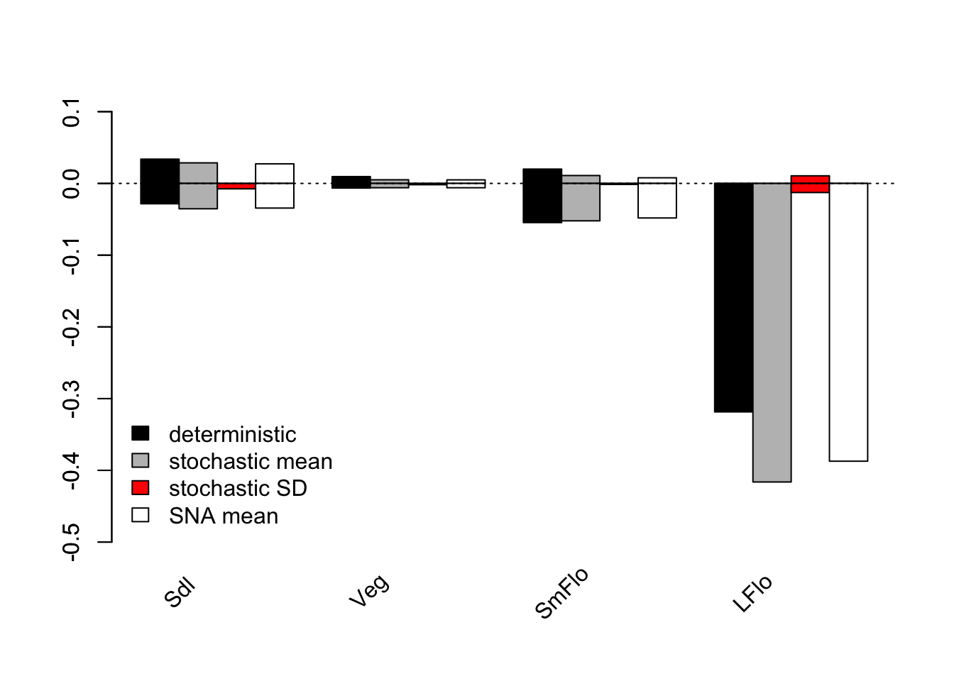
Figure 12.3: LTRE contributions by stage and LTRE type for population 1
Figure 12.3 shows that large flowering adults exerted the strongest influence on both \(\lambda\) and \(\text{log} \lambda\), with the latter influence being through the impact of shifts in the mean. This impact is overwhelmingly negative. The next largest impact comes from seedlings in the deterministic case, and from small flowering adults in the stochastic case, in both cases the influence being negative on the whole.
Finally, we will assess what transition types exert the greatest impact on population growth rate.
det_ltre_summary <- summary(trialltre_det)
sto_ltre_summary <- summary(trialltre_sto)
sna_ltre_summary <- summary(trialltre_sna)

ltresums_tpos <- cbind(det_ltre_summary$ahist_mean$matrix1_pos,
  sto_ltre_summary$ahist_mean$matrix1_pos,
  sto_ltre_summary$ahist_sd$matrix1_pos,
  sna_ltre_summary$ahist_mean$matrix1_pos)
ltresums_tneg <- cbind(det_ltre_summary$ahist_mean$matrix1_neg,
  sto_ltre_summary$ahist_mean$matrix1_neg,
  sto_ltre_summary$ahist_sd$matrix1_neg,
  sna_ltre_summary$ahist_mean$matrix1_neg)

barplot(t(ltresums_tpos), beside = T, col = c("black", "grey", "red", "white"),
  ylim = c(-0.55, 0.10))
barplot(t(ltresums_tneg), beside = T, col = c("black", "grey", "red", "white"),
  add = TRUE)
abline(0, 0, lty = 3)
text(cex=0.85, y = -0.64, x = seq(from = 2, to = 4.98*length(det_ltre_summary$ahist_mean$category),
    by = 5), det_ltre_summary$ahist_mean$category, xpd=TRUE, srt=45)
legend("bottomleft", fill = c("black", "grey", "red", "white"),
  legend = c("deterministic", "stochastic mean", "stochastic SD", "SNA mean"),
  bty = "n")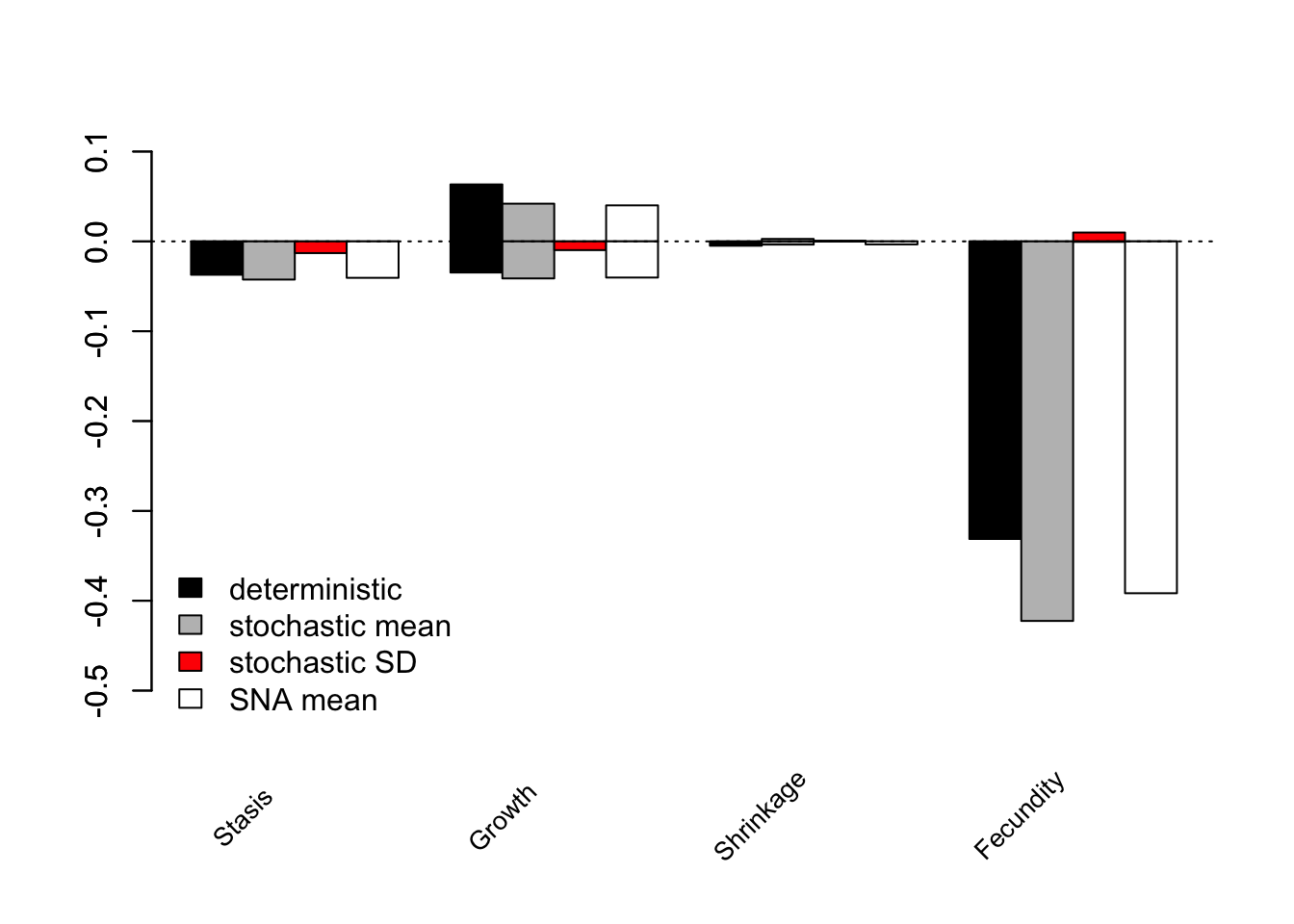
Figure 12.4: LTRE contributions by transition type and LTRE type
The overall greatest impact on the population growth rate was from fecundity transitions, which generally had a negative impact (figure 12.4). Clearly temporal variation had strong effects here that deserve to be assessed properly. Note that these impacts were relative to the grand mean.
12.5 Points to remember
- Life table response experiments (LTREs) allow the demographic impacts of specific factors to be tested, provided that the factors yield matrices that can be compared against some control. These analyses generally show the impacts of such factors on the deterministic or stochastic population growth growth rate via contributions from shifts in matrix elements.
- Stochastic life table response experiments (sLTREs) assess the impacts of factors on the stochastic population growth rate via shifts in both the temporal mean and the temporal standard deviation in matrix elements. Small noise approximation life table response experiments break down influences further to include the impacts of correlation among matrix elements, and elasticities of \(\lambda\) to shifts in matrix elements.
- LTRE contributions may be summed within matrices to assess the impacts of specific stages or transitions as they respond to some treatment.