Chapter 7 Matrix Models IV: Integral Projection Models
If people do not believe that mathematics is simple, it is only because they do not realize how complicated life is.
As seen in Chapter 5, MPMs may be estimated using functions representing vital rates, where these vital rate functions may then be used to estimate each matrix element. We term this the function-based MPM approach, because of its use of mathematical functions to estimate matrix elements. One reason that this approach is very powerful is that it allows population ecologists to create simulations in which vital rates themselves are manipulated, for example via altered climate relationships or management regimes.
Easterling et al. (2000) proposed a special case of the function-based MPM called the integral projection model (IPM). In integral projection models, the familiar projection equation \(\mathbf{n_{t+1}}=\mathbf{A} \mathbf{n_t}\) changes to the following.
\[\begin{equation} n(k, t+1) = \int_L^U K(k, j) n(j, t) dj \tag{7.1} \end{equation}\]
Here, an individual in state \(j\) in time \(t\) either transitions to state \(k\) or produces offspring in state \(k\) in time \(t+1\), \(n(j, t) dj\) refers to the number of individuals with their state in the range between \(j\) and \(j+dj\), \(L\) and \(U\) represent the lower and upper bounds of the state variable, and \(K(k, j)\) is the projection kernel \(K(k, j) = P(k, j) + F(k, j)\). In this projection kernel, \(P(k, j)\) represents the survival-transition probability from state \(j\) in time \(t\) to state \(k\) in time \(t+1\), and \(F(k, j)\) represents the production of offspring in state \(k\) in time \(t+1\) by an individual in state \(j\) in time \(t\). Because this equation is written as an integral as opposed to a discrete summation, it may appear to be quite different from the matrix approaches that we have seen so far. Indeed, there are those who have attempted to use these equations in their pure, integral forms, and when used analytically IPMs are not really MPMs. However, in practice, IPMs are typically discretized so that they may be parameterized as matrices. This discretization allows practitioners to use matrix approaches for analysis, because the projection kernel in equation (7.1) becomes perfectly analogous to the discrete projection equation \(\mathbf{n_{t+1}}=\mathbf{A} \mathbf{n_t}\).
Just as in other function-based MPMs, the IPM generally assumes that survival probabilities follow a binomial distribution and so may be estimated via generalized linear models, generalized linear mixed models, general additive models, or related approaches assuming a binomial response. Likewise, probabilities of reproduction, observation, or maturity, should also follow a binomial response. We see a difference in the estimation of the size probability, because IPMs require the use of a continuous size metric. In fact, the “traditional” IPM assumes a Gaussian distribution for size, and the underlying assumptions of the Gaussian distribution may fail in many circumstances and hence lead to biased results. A more flexible IPM approach allows the use of other distributions, including continuous distributions such as the gamma distribution, and discrete distributions such as the Poisson or negative binomial distributions when necessary. Package lefko3 allows all of these distributions.
Discretized IPMs assume vital rate models that parameterize the main kernel populating the matrix elements. These 14 vital rate models are described in chapter 5, and in section 5.1.
Of these fourteen vital rates, most users will estimate at least parameters (1) survival probability, (3) primary size transition probability, and (7) fecundity rate. These three are the default set for function modelsearch(). Parameters (2) observation probability and (6) reproduction probability may be used when some stages are included that are completely unobservable (and so do not have any size), or that are mature but non-reproductive, respectively. Parameters (4) secondary size transition and (5) tertiary size transition should only be used when size classification involves more than one size variable. Parameters (8) through (14) should only be added if the dataset contains juvenile individuals transitioning to maturity, and these juveniles live essentially as a single juvenile stage for some amount of time before transitioning to maturity, or before transitioning to a stage that is size-classified in the same manner as adult stages are. If juveniles can be classified by size similarly to adults (or at least on the same scale), then only vital rates (1) through (7) should be used and stage groups can be used with supplement tables to disallow transitions back to juvenile stages. If multiple juvenile stages exist on a different size classification system than adults, then stage groups may also be included as categorical variables in linear vital rate modeling in rates (1) through (7) to stratify vital rate models properly.
Let us assume that the state of the individual is represented by a continuous variable, such as a continuous size metric. This continuous size metric will be used to estimate parameter (3), the primary size transition probability. It may be Gaussian distributed, as is often assumed in IPMs (Doak et al. 2021), or may follow a different continuous distribution such as the gamma distribution. The survival-transition kernel \(P(k, j)\) and the fecundity kernel \(F(k, j)\) will be estimated as in the function-based MPM, as products of conditional rates or probabilities that are themselves estimated via linear models, additive models, or some other function-based approach. How, then, is the primary size transition probability estimated?
In practice, the range of the continuous state variable is broken down into a series of continuous domains, each with its own midpoint and upper and lower bounds. Individual domains under the Gaussian and gamma distributions are shown in figure 7.1 a and d, respectively. The domain midpoints are sometimes referred to as mesh points. Together with their upper and lower bounds they compose a series of size bins of generally equal size. To approximate a continuous size, we choose a rather high number of size bins, \(m\), perhaps on the order of 100 or even more.
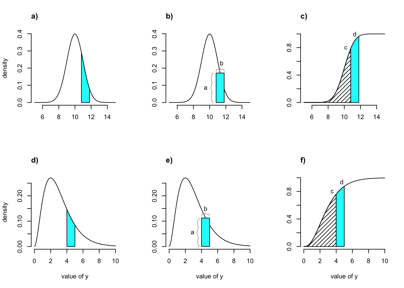
Figure 7.1: Shaded regions indicate the true size transition probability involved in transition (a,d), the estimated size transition probability via the midpoint method (b,e), and the estimated size transition probability via CDF (c,f) for the Gaussian (a-c) and gamma (d-f) distributions.
7.1 Midpoint method vs. cumulative density function (CDF)
There are several methods to estimate the size transition probabilities associated with each size bin. The original method developed is referred to as the midpoint method (Doak et al. 2021). It is the default in packages such as IPMpack and in some published guides to IPM creation (Metcalf et al. 2013; Merow et al. 2014). In the midpoint method, the mesh points are defined as \(j_i = L + (i - 0.5)h\), where \(i\) is the set of integers from 1 to \(m\) (\(i=1,2,...,m\)), \(m\) is the number of size bins to be used, \(L\) is the lower state bound as before, and \(h\) is the width of the state bin or size bin, given as \(h=(U-L)/m\). If each kernel is composed of a vital rate function assuming some sort of probability distribution, and size is distributed on a Gaussian, gamma, or other continuous distribution, then \(h\) accounts for the area under the distribution density curve for the corresponding vital rate contributing to the kernel at each midpoint size value used in the model (figure 7.1 b and e). If we think of the integral as being approximated by a series of rectangles under the function being integrated, then \(h\) accounts for the width of the rectangle in the area approximation. Thus, we have the following.
\[\begin{equation} n(x_j, t+1) = h \sum_{i=1}^m K(x_j, x_i) n(x_i, t) \tag{7.2} \end{equation}\]
Doak et al. (2021) pointed out that the midpoint method yields biased results, often overestimating size transition probabilities. They proposed a different method based on the cumulative density function associated with the continuous distribution being used. We will call this the CDF method. In this approach, the cumulative probabilities associated with the lower and higher boundaries of the size bin are first calculated. Then, the cumulative probability associated with the lower boundary is subtracted from that associated with the higher boundary, yielding the exact probability associated with the size bin itself (figure 7.1 c and f). This method does not yield biased results, and so is the default method used in lefko3 (although the midpoint method is available as an option).
The practical impact of both approaches is that a stageframe with size bins is required, just as in the function-based approach. If we have created size bins, then we have essentially created size-classified life history stages. Thus, equation (7.2) can be treated as a matrix projection, analogous to \(\mathbf{n_{t+1}}=\mathbf{Kn_t}\). So from a practical standpoint, an integral projection model is simply a function-based matrix projection model in which a continuous size metric determines demography. Indeed, Ellner & Rees (2006) further proposed a generalization allowing IPMs to be developed with some discrete stages in the life history, referring to this as the complex integral projection model. In practice, there is now virtually no difference between IPMs and function-based MPMs, although there are theoretical differences due to the assumption of integrals over continuous size in the former.
7.2 Creating IPMs
How do we create IPMs in package lefko3? This turns out to be quite easy. To illustrate the process, we will use the Lathyrus vernus dataset (see section 1.8.2). In this exercise, we will create both ahistorical and historical IPMs.
First, let’s take a look at the dataset.
data(lathyrus)
summary(lathyrus)
>     SUBPLOT          GENET          Volume88         lnVol88
>  Min.   :1.000   Min.   :  1.0   Min.   :   3.4   Min.   :1.200
>  1st Qu.:2.000   1st Qu.: 48.0   1st Qu.:  63.0   1st Qu.:4.100
>  Median :3.000   Median : 97.0   Median : 732.5   Median :6.600
>  Mean   :3.223   Mean   :110.2   Mean   : 749.4   Mean   :5.538
>  3rd Qu.:4.000   3rd Qu.:167.5   3rd Qu.:1025.5   3rd Qu.:6.900
>  Max.   :6.000   Max.   :284.0   Max.   :7032.0   Max.   :8.900
>                                  NA's   :404      NA's   :404
>     FCODE88           Flow88       Intactseed88 Dead1988       Dormant1988
>  Min.   :0.0000   Min.   : 1.00   Min.   : 0    Mode:logical   Mode:logical
>  1st Qu.:0.0000   1st Qu.: 4.00   1st Qu.: 0    NA's:1119      NA's:1119
>  Median :0.0000   Median : 8.00   Median : 0
>  Mean   :0.3399   Mean   :11.86   Mean   : 3
>  3rd Qu.:1.0000   3rd Qu.:15.00   3rd Qu.: 4
>  Max.   :1.0000   Max.   :66.00   Max.   :34
>  NA's   :404      NA's   :910     NA's   :875
>  Missing1988     Seedling1988      Volume89         lnVol89
>  Mode:logical   Min.   :1.000   Min.   :   1.8   Min.   :0.600
>  NA's:1119      1st Qu.:2.000   1st Qu.:  15.6   1st Qu.:2.700
>                 Median :2.000   Median : 118.8   Median :4.800
>                 Mean   :2.144   Mean   : 573.3   Mean   :4.855
>                 3rd Qu.:3.000   3rd Qu.: 968.8   3rd Qu.:6.900
>                 Max.   :3.000   Max.   :6539.4   Max.   :8.800
>                 NA's   :1022    NA's   :294      NA's   :294
>     FCODE89           Flow89       Intactseed89       Dead1989
>  Min.   :0.0000   Min.   : 1.00   Min.   : 0.000   Min.   :1
>  1st Qu.:0.0000   1st Qu.: 5.00   1st Qu.: 0.000   1st Qu.:1
>  Median :0.0000   Median :11.00   Median : 5.000   Median :1
>  Mean   :0.2667   Mean   :14.88   Mean   : 8.273   Mean   :1
>  3rd Qu.:1.0000   3rd Qu.:20.00   3rd Qu.:13.000   3rd Qu.:1
>  Max.   :1.0000   Max.   :97.00   Max.   :66.000   Max.   :1
>  NA's   :294      NA's   :906     NA's   :899      NA's   :1077
>   Dormant1989    Missing1989    Seedling1989      Volume90         lnVol90
>  Min.   :1      Min.   :1      Min.   :1.000   Min.   :   2.1   Min.   :0.700
>  1st Qu.:1      1st Qu.:1      1st Qu.:2.000   1st Qu.:  12.6   1st Qu.:2.500
>  Median :1      Median :1      Median :2.000   Median :  61.0   Median :4.100
>  Mean   :1      Mean   :1      Mean   :2.136   Mean   : 244.1   Mean   :4.207
>  3rd Qu.:1      3rd Qu.:1      3rd Qu.:2.000   3rd Qu.: 295.2   3rd Qu.:5.700
>  Max.   :1      Max.   :1      Max.   :3.000   Max.   :4242.8   Max.   :8.400
>  NA's   :1046   NA's   :1112   NA's   :1001    NA's   :245      NA's   :245
>     FCODE90           Flow90        Intactseed90       Dead1990
>  Min.   :0.0000   Min.   : 1.000   Min.   : 0.000   Min.   :1
>  1st Qu.:0.0000   1st Qu.: 3.000   1st Qu.: 0.000   1st Qu.:1
>  Median :0.0000   Median : 6.000   Median : 0.000   Median :1
>  Mean   :0.1581   Mean   : 8.104   Mean   : 2.514   Mean   :1
>  3rd Qu.:0.0000   3rd Qu.:10.750   3rd Qu.: 1.000   3rd Qu.:1
>  Max.   :1.0000   Max.   :54.000   Max.   :37.000   Max.   :1
>  NA's   :246      NA's   :985      NA's   :981      NA's   :1007
>   Dormant1990    Missing1990    Seedling1990      Volume91         lnVol91
>  Min.   :1      Min.   :1      Min.   :1.000   Min.   :   4.0   Min.   :1.400
>  1st Qu.:1      1st Qu.:1      1st Qu.:2.000   1st Qu.:  12.0   1st Qu.:2.500
>  Median :1      Median :1      Median :2.000   Median : 118.5   Median :4.800
>  Mean   :1      Mean   :1      Mean   :2.186   Mean   : 418.7   Mean   :4.642
>  3rd Qu.:1      3rd Qu.:1      3rd Qu.:2.000   3rd Qu.: 689.7   3rd Qu.:6.500
>  Max.   :1      Max.   :1      Max.   :3.000   Max.   :6645.8   Max.   :8.800
>  NA's   :1054   NA's   :1105   NA's   :1049    NA's   :305      NA's   :305
>     FCODE91           Flow91       Intactseed91       Dead1991    Dormant1991
>  Min.   :0.0000   Min.   : 1.00   Min.   : 0.000   Min.   :1     Min.   :1
>  1st Qu.:0.0000   1st Qu.: 4.00   1st Qu.: 0.000   1st Qu.:1     1st Qu.:1
>  Median :0.0000   Median : 8.00   Median : 3.500   Median :1     Median :1
>  Mean   :0.2525   Mean   :11.12   Mean   : 5.805   Mean   :1     Mean   :1
>  3rd Qu.:1.0000   3rd Qu.:15.00   3rd Qu.:10.000   3rd Qu.:1     3rd Qu.:1
>  Max.   :1.0000   Max.   :48.00   Max.   :48.000   Max.   :1     Max.   :1
>  NA's   :307      NA's   :954     NA's   :919      NA's   :925   NA's   :1034
>   Missing1991    Seedling1991
>  Min.   :1      Min.   :1.000
>  1st Qu.:1      1st Qu.:2.000
>  Median :1      Median :2.000
>  Mean   :1      Mean   :1.973
>  3rd Qu.:1      3rd Qu.:2.000
>  Max.   :1      Max.   :3.000
>  NA's   :1095   NA's   :1082
This dataset includes information on 1119 individuals, so there are 1119 rows with data. There are 38 columns. The first two columns give identifying information about each individual (SUBPLOT refers to the patch, and GENET refers to individual identity), with each individual’s data entirely restricted to one row. This is followed by four sets of nine columns, each named VolumeXX, lnVolXX, FCODEXX, FlowXX, IntactseedXX, Dead19XX, DormantXX, Missing19XX, and SeedlingXX, where XX corresponds to the year of observation and with years organized consecutively. Thus, columns 3-11 refer to year 1988, columns 12-20 refer to year 1989, etc.
7.2.1 Developing stageframes for IPMs
First, we will create a stageframe for this dataset. We will base our stageframe on the life history model provided in Ehrlén (2000), but use a different size classification based on the log leaf volume to allow IPM construction and make all mature stages other than vegetative dormancy reproductive (figure 7.2). To make sure our life history model is accurate, let’s first explore the size distribution of adults.
adult_sizes_1988 <- lathyrus$lnVol88[which(is.na(lathyrus$Seedling1988))]
adult_sizes_1989 <- lathyrus$lnVol89[which(is.na(lathyrus$Seedling1989))]
adult_sizes_1990 <- lathyrus$lnVol90[which(is.na(lathyrus$Seedling1990))]
adult_sizes_1991 <- lathyrus$lnVol91[which(is.na(lathyrus$Seedling1991))]

adult_sizes <- c(adult_sizes_1988, adult_sizes_1989, adult_sizes_1990,
  adult_sizes_1991)

min(adult_sizes, na.rm = TRUE)
> [1] 0.7
max(adult_sizes, na.rm = TRUE)
> [1] 8.9
We see that adults range in log leaf volume from 0.7 to 8.9, and so we need our life history model to include these sizes, as below.
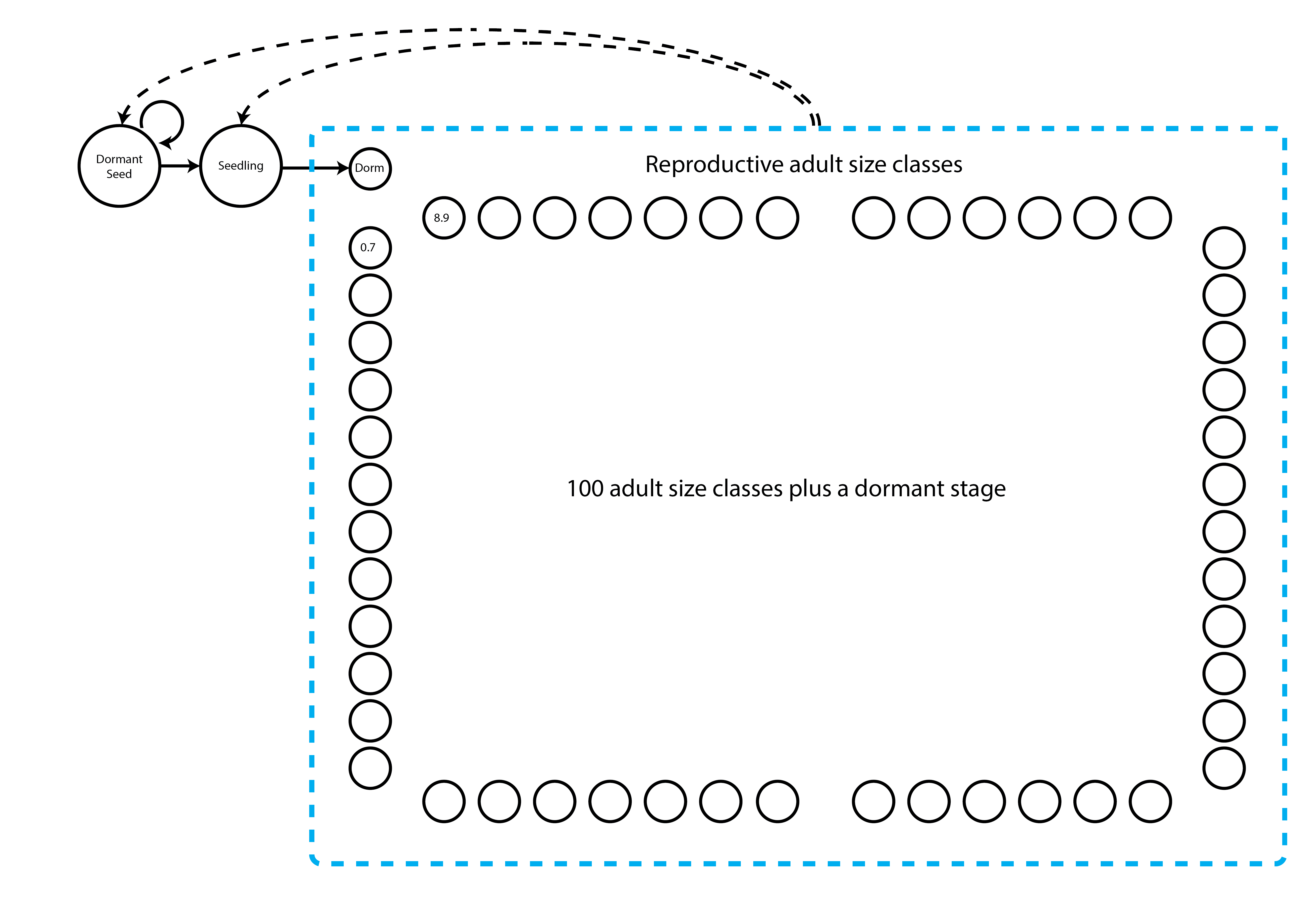
In the stageframe code below, we show that we want an IPM by choosing two stages that will serve as the minimum and maximum size limits for the range of the IPM’s discretized size variable(s). These two size classes should have exactly the same characteristics in the stageframe other than size. The size values input into the sizes vector for these two stages should not be midpoints. Instead, the size for the lower limit should be just a bit below the lower limit of the minimum size bin (since our minimum is 0.7, we will use 0.69), while the size input for the upper limit should be the upper limit of the maximum size bin (8.9). By choosing these two size limits, we can skip adding and describing the many size classes that will fall between these limits - function sf_create() will create all of these for us. We mark these limits in the vector that we load into the stagenames argument using the string "ipm". We then input all other characteristics for these size bins, including observation status, maturity status, and reproductive status. These characteristics must be the same for both the minimum and maximum size bins. Package lefko3 will then create and name all IPM size classes according to its own conventions. The default number of size classes is 100 bins, and this can be altered using the ipmbins option. Note that this is essentially the same procedure described in section 2.4.
sizevector <- c(0, 100, 0, 0.69, 8.9)
stagevector <- c("Sd", "Sdl", "Dorm", "ipm", "ipm")
repvector <- c(0, 0, 0, 1, 1)
obsvector <- c(0, 1, 0, 1, 1)
matvector <- c(0, 0, 1, 1, 1)
immvector <- c(1, 1, 0, 0, 0)
propvector <- c(1, 0, 0, 0, 0)
indataset <- c(0, 1, 1, 1, 1)
binvec <- c(0, 100, 0.5, 0.5, 0.5)
comments <- c("Dormant seed", "Seedling", "Dormant", "ipm adult stage",
  "ipm adult stage")

lathframeipm <- sf_create(sizes = sizevector, stagenames = stagevector,
  repstatus = repvector, obsstatus = obsvector, propstatus = propvector,
  immstatus = immvector, matstatus = matvector, comments = comments,
  indataset = indataset, binhalfwidth = binvec, ipmbins = 100, roundsize = 3)
> Warning: Values supplied in vectors sizemin, sizemax, and binhalfwidth will be overwritten for ipm bins.

dim(lathframeipm)
> [1] 103  29
This stageframe has 103 stages - dormant seed, seedling, vegetative dormancy, and 100 size-classified adult stages. Let’s look at just a few key columns.
lathframeipm[,c("stage", "size", "sizebin_min", "sizebin_max", "comments")]
>            stage      size sizebin_min sizebin_max        comments
> 1             Sd   0.00000       0.000       0.000    Dormant seed
> 2            Sdl 100.00000       0.000     200.000        Seedling
> 3           Dorm   0.00000      -0.500       0.500         Dormant
> 4   sza_0.7310_0   0.73105       0.690       0.772 ipm adult stage
> 5   sza_0.8131_0   0.81315       0.772       0.854 ipm adult stage
> 6   sza_0.8952_0   0.89525       0.854       0.936 ipm adult stage
> 7   sza_0.9773_0   0.97735       0.936       1.018 ipm adult stage
> 8   sza_1.0594_0   1.05945       1.018       1.100 ipm adult stage
> 9   sza_1.1415_0   1.14155       1.100       1.183 ipm adult stage
> 10  sza_1.2236_0   1.22365       1.183       1.265 ipm adult stage
> 11  sza_1.3057_0   1.30575       1.265       1.347 ipm adult stage
> 12  sza_1.3878_0   1.38785       1.347       1.429 ipm adult stage
> 13  sza_1.4699_0   1.46995       1.429       1.511 ipm adult stage
> 14  sza_1.5520_0   1.55205       1.511       1.593 ipm adult stage
> 15  sza_1.6341_0   1.63415       1.593       1.675 ipm adult stage
> 16  sza_1.7162_0   1.71625       1.675       1.757 ipm adult stage
> 17  sza_1.7983_0   1.79835       1.757       1.839 ipm adult stage
> 18  sza_1.8804_0   1.88045       1.839       1.922 ipm adult stage
> 19  sza_1.9625_0   1.96255       1.922       2.004 ipm adult stage
> 20  sza_2.0446_0   2.04465       2.004       2.086 ipm adult stage
> 21  sza_2.1267_0   2.12675       2.086       2.168 ipm adult stage
> 22  sza_2.2088_0   2.20885       2.168       2.250 ipm adult stage
> 23  sza_2.2909_0   2.29095       2.250       2.332 ipm adult stage
> 24  sza_2.3730_0   2.37305       2.332       2.414 ipm adult stage
> 25  sza_2.4551_0   2.45515       2.414       2.496 ipm adult stage
> 26  sza_2.5372_0   2.53725       2.496       2.578 ipm adult stage
> 27  sza_2.6193_0   2.61935       2.578       2.660 ipm adult stage
> 28  sza_2.7014_0   2.70145       2.660       2.742 ipm adult stage
> 29  sza_2.7835_0   2.78355       2.743       2.825 ipm adult stage
> 30  sza_2.8656_0   2.86565       2.825       2.907 ipm adult stage
> 31  sza_2.9477_0   2.94775       2.907       2.989 ipm adult stage
> 32  sza_3.0298_0   3.02985       2.989       3.071 ipm adult stage
> 33  sza_3.1119_0   3.11195       3.071       3.153 ipm adult stage
> 34  sza_3.1940_0   3.19405       3.153       3.235 ipm adult stage
> 35  sza_3.2761_0   3.27615       3.235       3.317 ipm adult stage
> 36  sza_3.3582_0   3.35825       3.317       3.399 ipm adult stage
> 37  sza_3.4403_0   3.44035       3.399       3.481 ipm adult stage
> 38  sza_3.5224_0   3.52245       3.481       3.563 ipm adult stage
> 39  sza_3.6045_0   3.60455       3.564       3.646 ipm adult stage
> 40  sza_3.6866_0   3.68665       3.646       3.728 ipm adult stage
> 41  sza_3.7687_0   3.76875       3.728       3.810 ipm adult stage
> 42  sza_3.8508_0   3.85085       3.810       3.892 ipm adult stage
> 43  sza_3.9329_0   3.93295       3.892       3.974 ipm adult stage
> 44  sza_4.0150_0   4.01505       3.974       4.056 ipm adult stage
> 45  sza_4.0971_0   4.09715       4.056       4.138 ipm adult stage
> 46  sza_4.1792_0   4.17925       4.138       4.220 ipm adult stage
> 47  sza_4.2613_0   4.26135       4.220       4.302 ipm adult stage
> 48  sza_4.3434_0   4.34345       4.302       4.385 ipm adult stage
> 49  sza_4.4255_0   4.42555       4.384       4.467 ipm adult stage
> 50  sza_4.5076_0   4.50765       4.467       4.549 ipm adult stage
> 51  sza_4.5897_0   4.58975       4.549       4.631 ipm adult stage
> 52  sza_4.6718_0   4.67185       4.631       4.713 ipm adult stage
> 53  sza_4.7539_0   4.75395       4.713       4.795 ipm adult stage
> 54  sza_4.8360_0   4.83605       4.795       4.877 ipm adult stage
> 55  sza_4.9181_0   4.91815       4.877       4.959 ipm adult stage
> 56  sza_5.0002_0   5.00025       4.959       5.041 ipm adult stage
> 57  sza_5.0823_0   5.08235       5.041       5.123 ipm adult stage
> 58  sza_5.1644_0   5.16445       5.123       5.206 ipm adult stage
> 59  sza_5.2465_0   5.24655       5.206       5.288 ipm adult stage
> 60  sza_5.3286_0   5.32865       5.288       5.370 ipm adult stage
> 61  sza_5.4107_0   5.41075       5.370       5.452 ipm adult stage
> 62  sza_5.4928_0   5.49285       5.452       5.534 ipm adult stage
> 63  sza_5.5749_0   5.57495       5.534       5.616 ipm adult stage
> 64  sza_5.6570_0   5.65705       5.616       5.698 ipm adult stage
> 65  sza_5.7391_0   5.73915       5.698       5.780 ipm adult stage
> 66  sza_5.8212_0   5.82125       5.780       5.862 ipm adult stage
> 67  sza_5.9033_0   5.90335       5.862       5.944 ipm adult stage
> 68  sza_5.9854_0   5.98545       5.944       6.027 ipm adult stage
> 69  sza_6.0675_0   6.06755       6.027       6.109 ipm adult stage
> 70  sza_6.1496_0   6.14965       6.109       6.191 ipm adult stage
> 71  sza_6.2317_0   6.23175       6.191       6.273 ipm adult stage
> 72  sza_6.3138_0   6.31385       6.273       6.355 ipm adult stage
> 73  sza_6.3959_0   6.39595       6.355       6.437 ipm adult stage
> 74  sza_6.4780_0   6.47805       6.437       6.519 ipm adult stage
> 75  sza_6.5601_0   6.56015       6.519       6.601 ipm adult stage
> 76  sza_6.6422_0   6.64225       6.601       6.683 ipm adult stage
> 77  sza_6.7243_0   6.72435       6.683       6.765 ipm adult stage
> 78  sza_6.8064_0   6.80645       6.765       6.848 ipm adult stage
> 79  sza_6.8885_0   6.88855       6.848       6.930 ipm adult stage
> 80  sza_6.9706_0   6.97065       6.930       7.012 ipm adult stage
> 81  sza_7.0527_0   7.05275       7.012       7.094 ipm adult stage
> 82  sza_7.1348_0   7.13485       7.094       7.176 ipm adult stage
> 83  sza_7.2169_0   7.21695       7.176       7.258 ipm adult stage
> 84  sza_7.2990_0   7.29905       7.258       7.340 ipm adult stage
> 85  sza_7.3811_0   7.38115       7.340       7.422 ipm adult stage
> 86  sza_7.4632_0   7.46325       7.422       7.504 ipm adult stage
> 87  sza_7.5453_0   7.54535       7.504       7.586 ipm adult stage
> 88  sza_7.6274_0   7.62745       7.586       7.669 ipm adult stage
> 89  sza_7.7095_0   7.70955       7.669       7.751 ipm adult stage
> 90  sza_7.7916_0   7.79165       7.751       7.833 ipm adult stage
> 91  sza_7.8737_0   7.87375       7.833       7.915 ipm adult stage
> 92  sza_7.9558_0   7.95585       7.915       7.997 ipm adult stage
> 93  sza_8.0379_0   8.03795       7.997       8.079 ipm adult stage
> 94  sza_8.1200_0   8.12005       8.079       8.161 ipm adult stage
> 95  sza_8.2021_0   8.20215       8.161       8.243 ipm adult stage
> 96  sza_8.2842_0   8.28425       8.243       8.325 ipm adult stage
> 97  sza_8.3663_0   8.36635       8.325       8.407 ipm adult stage
> 98  sza_8.4484_0   8.44845       8.407       8.490 ipm adult stage
> 99  sza_8.5305_0   8.53055       8.490       8.572 ipm adult stage
> 100 sza_8.6126_0   8.61265       8.572       8.654 ipm adult stage
> 101 sza_8.6947_0   8.69475       8.654       8.736 ipm adult stage
> 102 sza_8.7768_0   8.77685       8.736       8.818 ipm adult stage
> 103 sza_8.8589_0   8.85895       8.818       8.900 ipm adult stage
The function sf_create() has created our mesh points and associated size bins. This is in addition to the discrete stages covering the dormant seed, seedling, and dormant adult stages. Of course, we could have made this even more complex. For example, we could have created two sets of stages to use as the upper and lower bounds of two sets of continuous size states that differ in some key characteristic, such as reproductive status. We also could have set up the IPM using two or three different size metrics and used the ipm option within each or only some of them. This function provides a great deal of flexibility and power to create truly complex life history models.
An important additional point to bear in mind in discretized IPM creation relates to the impact of extreme size classes. Users developing IPMs with size classes that go even slightly beyond the range of real sizes seen in the dataset may create conditons in which the resulting IPM includes unusual behavior not representative of the monitored population. This situation is refered to as eviction from the IPM (Williams et al. 2012). We advise great care to be taken in determining particularly the limits for each size variable utilized, as well as the resolution of the mesh determining size classes.
7.2.2 Formatting demographic data and testing distribution assumptions
Next, we will format the data into hfv format. Because this is an IPM, we need to estimate linear models of vital rates. This will require us either to fix or to remove NAs in size and fecundity, so we will set NAas0 = TRUE. We will also set NRasRep = TRUE because we will assume that all adult stages other than dormancy are reproductive, and there are mature individuals in the dataset that do not reproduce but need to be included in reproductive stages (setting this option to TRUE makes sure that non-reproductive individuals in potentially reproductive stages are assumed to be reproductive, although their actual fecundity is not altered). Finally, we will ignore patches marked in the dataset and estimate matrices only for the full population in order to preserve statistical power for vital rate modeling in historical IPM analysis.
In the input to verticalize3() below, we utilize a repeating pattern of variable names arranged in the same order for each monitoring occasion. This arrangement allows us to enter only the first variable in each set, as long as noyears and blocksize are set properly and no gaps or shuffles appear in the dataset. The data management functions that we have created for lefko3 do not require such repeating patterns, but they do make the required input in the function much shorter and more succinct. Note also that we will use a new individual identity variable that incorporates the patch identity (indiv_id), to prevent repeat individual identities across patches.
lathyrus$indiv_id <- paste(lathyrus$SUBPLOT, lathyrus$GENET)

lathvertipm <- verticalize3(lathyrus, noyears = 4, firstyear = 1988,
  individcol = "indiv_id", blocksize = 9, juvcol = "Seedling1988",
  sizeacol = "lnVol88", repstracol = "FCODE88", fecacol = "Intactseed88",
  deadacol = "Dead1988", nonobsacol = "Dormant1988", stageassign = lathframeipm,
  stagesize = "sizea", censorcol = "Missing1988", censorkeep = NA,
  censorRepeat = TRUE, censor = TRUE, NAas0 = TRUE, NRasRep = TRUE)

summary_hfv(lathvertipm, full = TRUE)
>
> This hfv dataset contains 2527 rows, 54 variables, 1 population,
> 1 patch, 1053 individuals, and 3 time steps.
>      rowid           popid             patchid            individ
>  Min.   :   1.0   Length:2527        Length:2527        Length:2527
>  1st Qu.: 237.0   Class :character   Class :character   Class :character
>  Median : 522.0   Mode  :character   Mode  :character   Mode  :character
>  Mean   : 537.3
>  3rd Qu.: 820.5
>  Max.   :1118.0
>      year2        firstseen       lastseen        obsage       obslifespan
>  Min.   :1988   Min.   :   0   Min.   :   0   Min.   :1.000   Min.   :0.000
>  1st Qu.:1988   1st Qu.:1988   1st Qu.:1991   1st Qu.:1.000   1st Qu.:2.000
>  Median :1989   Median :1988   Median :1991   Median :2.000   Median :3.000
>  Mean   :1989   Mean   :1979   Mean   :1981   Mean   :1.822   Mean   :2.437
>  3rd Qu.:1990   3rd Qu.:1988   3rd Qu.:1991   3rd Qu.:2.000   3rd Qu.:3.000
>  Max.   :1990   Max.   :1990   Max.   :1991   Max.   :3.000   Max.   :3.000
>      sizea1        size1added       repstra1       repstr1added
>  Min.   :0.000   Min.   :0.000   Min.   :0.0000   Min.   :0.0000
>  1st Qu.:0.000   1st Qu.:0.000   1st Qu.:0.0000   1st Qu.:0.0000
>  Median :2.200   Median :2.200   Median :0.0000   Median :0.0000
>  Mean   :2.957   Mean   :2.957   Mean   :0.1805   Mean   :0.1805
>  3rd Qu.:6.400   3rd Qu.:6.400   3rd Qu.:0.0000   3rd Qu.:0.0000
>  Max.   :8.900   Max.   :8.900   Max.   :1.0000   Max.   :1.0000
>      feca1          fec1added         censor1    juvgiven1
>  Min.   : 0.000   Min.   : 0.000   Min.   :0   Min.   :0.00000
>  1st Qu.: 0.000   1st Qu.: 0.000   1st Qu.:0   1st Qu.:0.00000
>  Median : 0.000   Median : 0.000   Median :0   Median :0.00000
>  Mean   : 0.989   Mean   : 0.989   Mean   :0   Mean   :0.06292
>  3rd Qu.: 0.000   3rd Qu.: 0.000   3rd Qu.:0   3rd Qu.:0.00000
>  Max.   :66.000   Max.   :66.000   Max.   :0   Max.   :1.00000
>    obsstatus1       repstatus1       fecstatus1        matstatus1
>  Min.   :0.0000   Min.   :0.0000   Min.   :0.00000   Min.   :0.0000
>  1st Qu.:0.0000   1st Qu.:0.0000   1st Qu.:0.00000   1st Qu.:0.0000
>  Median :1.0000   Median :0.0000   Median :0.00000   Median :1.0000
>  Mean   :0.5548   Mean   :0.1805   Mean   :0.08983   Mean   :0.5204
>  3rd Qu.:1.0000   3rd Qu.:0.0000   3rd Qu.:0.00000   3rd Qu.:1.0000
>  Max.   :1.0000   Max.   :1.0000   Max.   :1.00000   Max.   :1.0000
>      alive1          stage1           stage1index         sizea2
>  Min.   :0.0000   Length:2527        Min.   :  0.00   Min.   :0.000
>  1st Qu.:0.0000   Class :character   1st Qu.:  0.00   1st Qu.:2.500
>  Median :1.0000   Mode  :character   Median :  3.00   Median :4.700
>  Mean   :0.5833                      Mean   : 32.16   Mean   :4.565
>  3rd Qu.:1.0000                      3rd Qu.: 73.00   3rd Qu.:6.600
>  Max.   :1.0000                      Max.   :103.00   Max.   :8.900
>    size2added       repstra2      repstr2added       feca2
>  Min.   :0.000   Min.   :0.000   Min.   :0.000   Min.   : 0.00
>  1st Qu.:2.500   1st Qu.:0.000   1st Qu.:0.000   1st Qu.: 0.00
>  Median :4.700   Median :0.000   Median :0.000   Median : 0.00
>  Mean   :4.565   Mean   :0.237   Mean   :0.237   Mean   : 1.14
>  3rd Qu.:6.600   3rd Qu.:0.000   3rd Qu.:0.000   3rd Qu.: 0.00
>  Max.   :8.900   Max.   :1.000   Max.   :1.000   Max.   :66.00
>    fec2added        censor2    juvgiven2        obsstatus2       repstatus2
>  Min.   : 0.00   Min.   :0   Min.   :0.0000   Min.   :0.0000   Min.   :0.000
>  1st Qu.: 0.00   1st Qu.:0   1st Qu.:0.0000   1st Qu.:1.0000   1st Qu.:0.000
>  Median : 0.00   Median :0   Median :0.0000   Median :1.0000   Median :0.000
>  Mean   : 1.14   Mean   :0   Mean   :0.1112   Mean   :0.9454   Mean   :0.237
>  3rd Qu.: 0.00   3rd Qu.:0   3rd Qu.:0.0000   3rd Qu.:1.0000   3rd Qu.:0.000
>  Max.   :66.00   Max.   :0   Max.   :1.0000   Max.   :1.0000   Max.   :1.000
>    fecstatus2       matstatus2         alive2     stage2
>  Min.   :0.0000   Min.   :0.0000   Min.   :1   Length:2527
>  1st Qu.:0.0000   1st Qu.:1.0000   1st Qu.:1   Class :character
>  Median :0.0000   Median :1.0000   Median :1   Mode  :character
>  Mean   :0.1053   Mean   :0.8888   Mean   :1
>  3rd Qu.:0.0000   3rd Qu.:1.0000   3rd Qu.:1
>  Max.   :1.0000   Max.   :1.0000   Max.   :1
>   stage2index         sizea3        size3added       repstra3
>  Min.   :  2.00   Min.   :0.000   Min.   :0.000   Min.   :0.000
>  1st Qu.: 26.00   1st Qu.:2.300   1st Qu.:2.300   1st Qu.:0.000
>  Median : 52.00   Median :4.300   Median :4.300   Median :0.000
>  Mean   : 48.99   Mean   :4.043   Mean   :4.043   Mean   :0.218
>  3rd Qu.: 75.00   3rd Qu.:6.300   3rd Qu.:6.300   3rd Qu.:0.000
>  Max.   :103.00   Max.   :8.800   Max.   :8.800   Max.   :1.000
>   repstr3added       feca3         fec3added        censor3    juvgiven3
>  Min.   :0.000   Min.   : 0.00   Min.   : 0.00   Min.   :0   Min.   :0
>  1st Qu.:0.000   1st Qu.: 0.00   1st Qu.: 0.00   1st Qu.:0   1st Qu.:0
>  Median :0.000   Median : 0.00   Median : 0.00   Median :0   Median :0
>  Mean   :0.218   Mean   : 1.29   Mean   : 1.29   Mean   :0   Mean   :0
>  3rd Qu.:0.000   3rd Qu.: 0.00   3rd Qu.: 0.00   3rd Qu.:0   3rd Qu.:0
>  Max.   :1.000   Max.   :66.00   Max.   :66.00   Max.   :0   Max.   :0
>    obsstatus3       repstatus3      fecstatus3       matstatus3
>  Min.   :0.0000   Min.   :0.000   Min.   :0.0000   Min.   :1
>  1st Qu.:1.0000   1st Qu.:0.000   1st Qu.:0.0000   1st Qu.:1
>  Median :1.0000   Median :0.000   Median :0.0000   Median :1
>  Mean   :0.8346   Mean   :0.218   Mean   :0.1116   Mean   :1
>  3rd Qu.:1.0000   3rd Qu.:0.000   3rd Qu.:0.0000   3rd Qu.:1
>  Max.   :1.0000   Max.   :1.000   Max.   :1.0000   Max.   :1
>      alive3          stage3           stage3index
>  Min.   :0.0000   Length:2527        Min.   :  0.00
>  1st Qu.:1.0000   Class :character   1st Qu.: 23.00
>  Median :1.0000   Mode  :character   Median : 47.00
>  Mean   :0.9224                      Mean   : 45.43
>  3rd Qu.:1.0000                      3rd Qu.: 72.00
>  Max.   :1.0000                      Max.   :102.00
Before we move on to the next steps in analysis, let’s take a closer look at fecundity. In this dataset, fecundity is mostly a count of intact seeds, and only differs in six cases where the seed output was estimated based on other models. To see this, try the following code.
# Length of fecundity in t+1:
length(lathvertipm$feca3)
> [1] 2527
# Total non-integer entries in fecundity in occasion t+1:
length(which(lathvertipm$feca3 != round(lathvertipm$feca3)))
> [1] 0
# Length of fecundity in t:
length(lathvertipm$feca2)
> [1] 2527
# Total non-integer entries in fecundity in occasion t:
length(which(lathvertipm$feca2 != round(lathvertipm$feca2)))
> [1] 6
# Length of fecundity in t-1:
length(lathvertipm$feca1)
> [1] 2527
# Total non-integer entries in fecundity in occasion t-1:
length(which(lathvertipm$feca1 != round(lathvertipm$feca1)))
> [1] 6lathvertipm$feca3 <- round(lathvertipm$feca3)
lathvertipm$feca2 <- round(lathvertipm$feca2)
lathvertipm$feca1 <- round(lathvertipm$feca1)Let’s now look at size. Ideally, we would assume the Gaussian distribution for this continuous variable. Let’s view a density plot (figure 7.3).
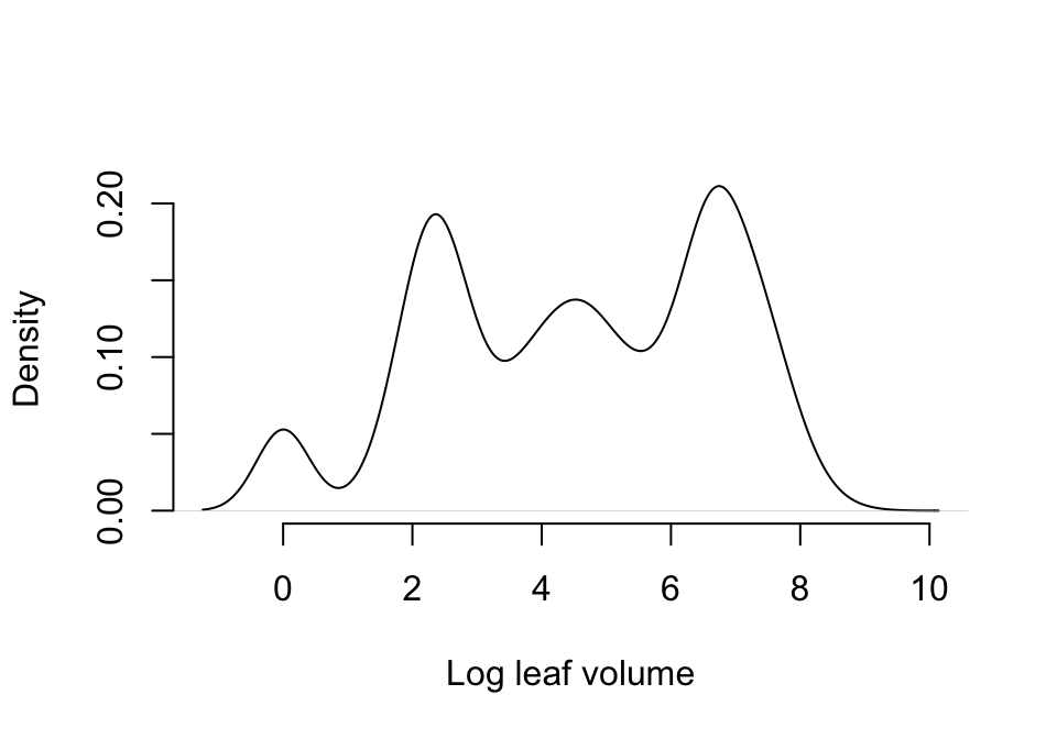
Figure 7.3: Probability density associated with primary size, unaltered
This distribution is quite odd, but perhaps close to symmetrical at least. We have absorbed the size of zero into the dormant stage, and the remaining sizes are all positive. So, we will try using the Gaussian distribution here.
Although we wish to treat fecundity as a count, it is still not clear what underlying distribution we should use. This package currently allows eight choices: Gaussian, gamma, Poisson, negative binomial, zero-inflated Poisson, zero-inflated negative binomial, zero-truncated Poisson, and zero-truncated negative binomial. To assess which to use, we should first assess whether the mean and variance of the count are equal using a dispersion test. The Poisson distribution assumes that the mean and variance are equal, and so we can test this assumption using a \(\chi ^2\) test. If it is not significantly different, then we may use some variant of the Poisson distribution. If the data are significantly overdispersed, then we should use the negative binomial distribution. If fecundity of zero is possible in reproductive stages, as in cases where reproductive status is defined by flowering rather than by offspring production, then we should also test whether the number of zeros is significantly greater than expected under these distributions, and use a zero-inflated distribution if so (if fecundity does not equal zero in any reproductive individuals at all, then we should use a zero-truncated distribution).
Let’s look at a plot of the distribution of fecundity (figure 7.4).
hist(subset(lathvertipm, repstatus2 == 1)$feca2, main = "Fecundity",
  xlab = expression(paste("Intact seeds produced in occasion ", italic(t))))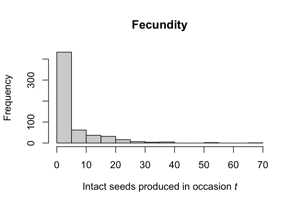
Figure 7.4: Histogram of fecundity
We see that the distribution seems to conform to a classic count variable with a very low mean value. The first bar suggests that there may be too many zeros to use a standard Poisson or negative binomial distribution. To make that decision, let’s formally test the assumptions that the mean equals the variance, and that there are not excess zeros. Both tests use \(\chi ^2\) distribution-based approaches, with the zero-inflation test based on Broek (1995). This is done automatically via the hfv_qc() function.
hfv_qc(lathvertipm, vitalrates = c("surv", "obs", "size", "fec"),
  juvestimate = "Sdl", indiv = "individ", year = "year2")
> Survival:
>
>   Data subset has 54 variables and 2246 transitions.
>
>   Variable alive3 has 0 missing values.
>   Variable alive3 is a binomial variable.
>
>   Numbers of categories in data subset in possible random variables:
>   indiv id: 931   (singleton categories: 181)
>   year2: 3   (singleton categories: 0)
>
> Observation status:
>
>   Data subset has 54 variables and 2121 transitions.
>
>   Variable obsstatus3 has 0 missing values.
>   Variable obsstatus3 is a binomial variable.
>
>   Numbers of categories in data subset in possible random variables:
>   indiv id: 858   (singleton categories: 143)
>   year2: 3   (singleton categories: 0)
>
> Primary size:
>
>   Data subset has 54 variables and 1916 transitions.
>
>   Variable sizea3 has 0 missing values.
>   Variable sizea3 appears to be a floating point variable.
>   1753 elements are not integers.
>   The minimum value of sizea3 is 1.2 and the maximum is 8.8.
>   The mean value of sizea3 is 5.099 and the variance is 3.093.
>   The value of the Shapiro-Wilk test of normality is 0.9551 with P = 7.719e-24.
>   Variable sizea3 differs significantly from a Gaussian distribution.
>
>   Variable sizea3 is fully positive, lacking even 0s.
>
>   Numbers of categories in data subset in possible random variables:
>   indiv id: 845   (singleton categories: 185)
>   year2: 3   (singleton categories: 0)
>
> Fecundity:
>
>   Data subset has 54 variables and 2246 transitions.
>
>   Variable feca2 has 0 missing values.
>   Variable feca2 appears to be an integer variable.
>
>   Variable feca2 is fully non-negative.
>
>   Overdispersion test:
>     Mean feca2 is 1.282
>     The variance in feca2 is 23.21
>     The probability of this dispersion level by chance assuming that
>     the true mean feca2 = variance in feca2,
>     and an alternative hypothesis of overdispersion, is 0
>     Variable feca2 is significantly overdispersed.
>
>   Zero-inflation and truncation tests:
>     Mean lambda in feca2 is 0.2774
>     The actual number of 0s in feca2 is 1980
>     The expected number of 0s in feca2 under the null hypothesis is 623
>     The probability of this deviation in 0s from expectation by chance is 0
>     Variable feca2 is significantly zero-inflated.
>
>   Numbers of categories in data subset in possible random variables:
>   indiv id: 931   (singleton categories: 181)
>   year2: 3   (singleton categories: 0)
>
> Juvenile survival:
>
>   Data subset has 54 variables and 281 transitions.
>
>   Variable alive3 has 0 missing values.
>   Variable alive3 is a binomial variable.
>
>   Numbers of categories in data subset in possible random variables:
>   indiv id: 281   (singleton categories: 281)
>   year2: 3   (singleton categories: 0)
>
> Juvenile observation status:
>
>   Data subset has 54 variables and 210 transitions.
>
>   Variable obsstatus3 has 0 missing values.
>   Variable obsstatus3 is a binomial variable.
>
>   Numbers of categories in data subset in possible random variables:
>   indiv id: 210   (singleton categories: 210)
>   year2: 3   (singleton categories: 0)
>
> Juvenile primary size:
>
>   Data subset has 54 variables and 193 transitions.
>
>   Variable sizea3 has 0 missing values.
>   Variable sizea3 appears to be a floating point variable.
>   183 elements are not integers.
>   The minimum value of sizea3 is 0.7 and the maximum is 4.1.
>   The mean value of sizea3 is 2.307 and the variance is 0.2051.
>   The value of the Shapiro-Wilk test of normality is 0.9273 with P = 3.278e-08.
>   Variable sizea3 differs significantly from a Gaussian distribution.
>
>   Variable sizea3 is fully positive, lacking even 0s.
>
>   Numbers of categories in data subset in possible random variables:
>   indiv id: 193   (singleton categories: 193)
>   year2: 3   (singleton categories: 0)
>
> Juvenile maturity status:
>
>   Data subset has 54 variables and 210 transitions.
>
>   Variable matstatus3 has 0 missing values.
>   Variable matstatus3 is a binomial variable.
>
>   Numbers of categories in data subset in possible random variables:
>   indiv id: 210   (singleton categories: 210)
>   year2: 3   (singleton categories: 0)
Such significant results for both tests under the fecundity heading show us that we should use a zero-inflated negative binomial distribution for fecundity. We also see that we might have problems modeling the juvenile rates with mixed models, since each individual corresponds to a single row in that dataset. This will likely make it impossible to treat individual identity as random in those models.
Now we will create supplement tables to provide extra data for matrix estimation that is not included in the main demographic dataset. Specifically, we will provide the seed dormancy probability and germination rate, which are given as transitions from the dormant seed stage to another year of seed dormancy or to the germinated seedling stage, respectively. We assume that the germination rate is the same regardless of whether seed was produced in the previous year or has been in the seedbank for longer. We will incorporate these terms both as fixed constants for specific transitions within the resulting matrices, and as multipliers for fecundity, since ultimately fecundity will be estimated as the production of seed multiplied by the seed germination rate or the seed dormancy rate. Because some individuals stay in the seedling stage for only one year, and the seed stage itself cannot be observed and so does not exist in the dataset, we will also set a proxy set of transitions so that R assumes that the transitions from seed in occasion t-1 to seedling in occasion t to all mature stages in occasion t+1 are equal to the equivalent transitions from seedling in both occasions t-1 and t.
We will start with the ahistorical case, and then move on to the historical case, where we also need to input the corresponding stages in occasion t-1 and transition types from occasion t-1 to t for each transition. Note the use of the "rep", "mat", and "npr" designations in Stage1 - these are abbreviations telling R to use all reproductive stages, all mature stages, or all non-propagule stages (mature stages plus the seedling stage) in general, respectively.
lathsupp2 <- supplemental(stage3 = c("Sd", "Sdl", "Sd", "Sdl"),
  stage2 = c("Sd", "Sd", "rep", "rep"),
  givenrate = c(0.345, 0.054, NA, NA),
  multiplier = c(NA, NA, 0.345, 0.054),
  type = c(1, 1, 3, 3), stageframe = lathframeipm, historical = FALSE)
> Warning: NA values in argument multiplier will be treated as 1 values.

lathsupp3 <- supplemental(stage3 = c("Sd","Sd","Sdl","Sdl","npr","Sd","Sdl"),
  stage2 = c("Sd", "Sd", "Sd", "Sd", "Sdl", "rep", "rep"),
  stage1 = c("Sd", "rep", "Sd", "rep", "Sd", "mat", "mat"),
  eststage3 = c(NA, NA, NA, NA, "npr", NA, NA),
  eststage2 = c(NA, NA, NA, NA, "Sdl", NA, NA),
  eststage1 = c(NA, NA, NA, NA, "Sdl", NA, NA),
  givenrate = c(0.345, 0.345, 0.054, 0.054, NA, NA, NA),
  multiplier = c(NA, NA, NA, NA, NA, 0.345, 0.054),
  type = c(1, 1, 1, 1, 1, 3, 3), type_t12 = c(1, 2, 1, 2, 1, 1, 1),
  stageframe = lathframeipm, historical = TRUE)
> Warning: NA values in argument multiplier will be treated as 1 values.

lathsupp2
>   stage3 stage2 stage1 age2 eststage3 eststage2 eststage1 estage2 givenrate
> 1     Sd     Sd   <NA>   NA      <NA>      <NA>      <NA>      NA     0.345
> 2    Sdl     Sd   <NA>   NA      <NA>      <NA>      <NA>      NA     0.054
> 3     Sd    rep   <NA>   NA      <NA>      <NA>      <NA>      NA        NA
> 4    Sdl    rep   <NA>   NA      <NA>      <NA>      <NA>      NA        NA
>   offset multiplier convtype convtype_t12
> 1     NA      1.000        1            1
> 2     NA      1.000        1            1
> 3     NA      0.345        3            1
> 4     NA      0.054        3            1
lathsupp3
>   stage3 stage2 stage1 age2 eststage3 eststage2 eststage1 estage2 givenrate
> 1     Sd     Sd     Sd   NA      <NA>      <NA>      <NA>      NA     0.345
> 2     Sd     Sd    rep   NA      <NA>      <NA>      <NA>      NA     0.345
> 3    Sdl     Sd     Sd   NA      <NA>      <NA>      <NA>      NA     0.054
> 4    Sdl     Sd    rep   NA      <NA>      <NA>      <NA>      NA     0.054
> 5    npr    Sdl     Sd   NA       npr       Sdl       Sdl      NA        NA
> 6     Sd    rep    mat   NA      <NA>      <NA>      <NA>      NA        NA
> 7    Sdl    rep    mat   NA      <NA>      <NA>      <NA>      NA        NA
>   offset multiplier convtype convtype_t12
> 1     NA      1.000        1            1
> 2     NA      1.000        1            2
> 3     NA      1.000        1            1
> 4     NA      1.000        1            2
> 5     NA      1.000        1            1
> 6     NA      0.345        3            1
> 7     NA      0.054        3            1
7.2.3 Estimating vital rate models
Integral projection models require functions of vital rates to populate them. Here, we will develop these functions as linear models using modelsearch(). First, we will create the historical models to assess whether history is a significant influence on vital rates. Note that we have set the appropriate size and fecundity distributions through the settings sizedist = "Gaussian", fecdist = "negbin", and fec.zero = TRUE. We will also set suite = "size", because our stageframe assumes that all sprouting stages are essentially reproductive. Thus, we cannot test the influence of reproductive status on vital rates since the resulting matrices will not have separate stages for reproductive vs. non-reproductive individuals.
lathmodels3ipm <- modelsearch(lathvertipm, historical = TRUE, approach= "mixed",
  suite = "size", vitalrates = c("surv", "obs", "size", "fec"),
  juvestimate = "Sdl", bestfit = "AICc&k", sizedist = "Gaussian",
  fecdist = "negbin", fec.zero = TRUE, indiv = "individ", year = "year2",
  year.as.random = TRUE, juvsize = TRUE, show.model.tables = TRUE,
  quiet = "partial")
Now let’s see a summary.
summary(lathmodels3ipm)
> This LefkoMod object includes 7 linear models.
> Best-fit model criterion used: aicc&k
>
>
>
> Survival model:
> Generalized linear mixed model fit by maximum likelihood (Laplace
>   Approximation) [glmerMod]
>  Family: binomial  ( logit )
> Formula: alive3 ~ (1 | year2) + (1 | individ)
>    Data: surv.data
>       AIC       BIC    logLik -2*log(L)  df.resid
>  709.9383  727.0890 -351.9691  703.9383      2243
> Random effects:
>  Groups  Name        Std.Dev.
>  individ (Intercept) 14.6
>  year2   (Intercept)  0.0
> Number of obs: 2246, groups:  individ, 931; year2, 3
> Fixed Effects:
> (Intercept)
>       10.03
> optimizer (Nelder_Mead) convergence code: 0 (OK) ; 0 optimizer warnings; 1 lme4 warnings
>
>
>
> Observation model:
> Generalized linear mixed model fit by maximum likelihood (Laplace
>   Approximation) [glmerMod]
>  Family: binomial  ( logit )
> Formula: obsstatus3 ~ sizea1 + sizea2 + (1 | year2) + (1 | individ)
>    Data: obs.data
>       AIC       BIC    logLik -2*log(L)  df.resid
>  1305.000  1333.298  -647.500  1295.000      2116
> Random effects:
>  Groups  Name        Std.Dev.
>  individ (Intercept) 9.194
>  year2   (Intercept) 0.000
> Number of obs: 2121, groups:  individ, 858; year2, 3
> Fixed Effects:
> (Intercept)       sizea1       sizea2
>     14.5041      -0.3982      -0.7603
> optimizer (Nelder_Mead) convergence code: 0 (OK) ; 0 optimizer warnings; 1 lme4 warnings
>
>
>
> Size model:
> Linear mixed model fit by REML ['lmerMod']
> Formula: sizea3 ~ sizea1 + sizea2 + (1 | year2) + (1 | individ)
>    Data: size.data
> REML criterion at convergence: 5574.663
> Random effects:
>  Groups   Name        Std.Dev.
>  individ  (Intercept) 0.9540
>  year2    (Intercept) 0.8348
>  Residual             0.7345
> Number of obs: 1916, groups:  individ, 845; year2, 3
> Fixed Effects:
> (Intercept)       sizea1       sizea2
>      2.9853       0.1877       0.3053
>
>
>
> Secondary size model:
> [1] 1
>
>
>
> Tertiary size model:
> [1] 1
>
>
>
> Reproductive status model:
> [1] 1
>
>
>
> Fecundity model:
> Formula:          feca2 ~ sizea1 + sizea2 + (1 | year2) + (1 | individ)
> Zero inflation:         ~sizea2 + (1 | year2) + (1 | individ)
> Data: fec.data
>       AIC       BIC    logLik -2*log(L)  df.resid
>  2742.162  2799.331 -1361.081  2722.162      2236
> Random-effects (co)variances:
>
> Conditional model:
>  Groups  Name        Std.Dev.
>  year2   (Intercept) 0.0005792
>  individ (Intercept) 0.3593252
>
> Zero-inflation model:
>  Groups  Name        Std.Dev.
>  year2   (Intercept) 0.4825
>  individ (Intercept) 0.6339
>
> Number of obs: 2246 / Conditional model: year2, 3; individ, 931 / Zero-inflation model: year2, 3; individ, 931
>
> Dispersion parameter for nbinom2 family (): 2.73
>
> Fixed Effects:
>
> Conditional model:
> (Intercept)       sizea1       sizea2
>    -1.98336      0.03804      0.55832
>
> Zero-inflation model:
> (Intercept)       sizea2
>      12.958       -1.701
>
>
> Juvenile survival model:
> Generalized linear mixed model fit by maximum likelihood (Laplace
>   Approximation) [glmerMod]
>  Family: binomial  ( logit )
> Formula: alive3 ~ (1 | year2) + (1 | individ)
>    Data: juvsurv.data
>       AIC       BIC    logLik -2*log(L)  df.resid
>  323.6696  334.5847 -158.8348  317.6696       278
> Random effects:
>  Groups  Name        Std.Dev.
>  individ (Intercept) 2.924e-05
>  year2   (Intercept) 0.000e+00
> Number of obs: 281, groups:  individ, 281; year2, 3
> Fixed Effects:
> (Intercept)
>       1.084
> optimizer (Nelder_Mead) convergence code: 0 (OK) ; 0 optimizer warnings; 1 lme4 warnings
>
>
>
> Juvenile observation model:
> Generalized linear mixed model fit by maximum likelihood (Laplace
>   Approximation) [glmerMod]
>  Family: binomial  ( logit )
> Formula: obsstatus3 ~ sizea2 + (1 | year2) + (1 | individ)
>    Data: juvobs.data
>       AIC       BIC    logLik -2*log(L)  df.resid
>   61.3610   74.7495  -26.6805   53.3610       206
> Random effects:
>  Groups  Name        Std.Dev.
>  individ (Intercept) 52.8210
>  year2   (Intercept)  0.1879
> Number of obs: 210, groups:  individ, 210; year2, 3
> Fixed Effects:
> (Intercept)       sizea2
>     11.7595       0.6446
>
>
>
> Juvenile size model:
> Linear mixed model fit by REML ['lmerMod']
> Formula: sizea3 ~ sizea2 + (1 | year2)
>    Data: juvsize.data
> REML criterion at convergence: 194.2248
> Random effects:
>  Groups   Name        Std.Dev.
>  year2    (Intercept) 0.1589
>  Residual             0.3888
> Number of obs: 193, groups:  year2, 3
> Fixed Effects:
> (Intercept)       sizea2
>      0.8252       0.6750
>
>
>
> Juvenile secondary size model:
> [1] 1
>
>
>
> Juvenile tertiary size model:
> [1] 1
>
>
>
> Juvenile reproduction model:
> [1] 1
>
>
>
> Juvenile maturity model:
> [1] 1
>
>
>
>
>
> Number of models in survival table: 3
>
> Number of models in observation table: 4
>
> Number of models in size table: 4
>
> Number of models in secondary size table: 1
>
> Number of models in tertiary size table: 1
>
> Number of models in reproduction status table: 1
>
> Number of models in fecundity table: 16
>
> Number of models in juvenile survival table: 2
>
> Number of models in juvenile observation table: 2
>
> Number of models in juvenile size table: 2
>
> Number of models in juvenile secondary size table: 1
>
> Number of models in juvenile tertiary size table: 1
>
> Number of models in juvenile reproduction table: 1
>
> Number of models in juvenile maturity table: 1
>
>
>
>
>
> General model parameter names (column 1), and
> specific names used in these models (column 2):
>                       parameter_names mainparams
> 1                              time t      year2
> 2                          individual    individ
> 3                               patch      patch
> 4                   alive in time t+1      surv3
> 5                observed in time t+1       obs3
> 6                   sizea in time t+1      size3
> 7                   sizeb in time t+1     sizeb3
> 8                   sizec in time t+1     sizec3
> 9     reproductive status in time t+1     repst3
> 10              fecundity in time t+1       fec3
> 11                fecundity in time t       fec2
> 12                    sizea in time t      size2
> 13                  sizea in time t-1      size1
> 14                    sizeb in time t     sizeb2
> 15                  sizeb in time t-1     sizeb1
> 16                    sizec in time t     sizec2
> 17                  sizec in time t-1     sizec1
> 18      reproductive status in time t     repst2
> 19    reproductive status in time t-1     repst1
> 20        maturity status in time t+1     matst3
> 21          maturity status in time t     matst2
> 22                      age in time t        age
> 23                  density in time t    density
> 24   individual covariate a in time t   indcova2
> 25 individual covariate a in time t-1   indcova1
> 26   individual covariate b in time t   indcovb2
> 27 individual covariate b in time t-1   indcovb1
> 28   individual covariate c in time t   indcovc2
> 29 individual covariate c in time t-1   indcovc1
> 30              stage group in time t     group2
> 31            stage group in time t-1     group1
> 32       annual covariate a in time t  annucova2
> 33     annual covariate a in time t-1  annucova1
> 34       annual covariate b in time t  annucovb2
> 35     annual covariate b in time t-1  annucovb1
> 36       annual covariate c in time t  annucovc2
> 37     annual covariate c in time t-1  annucovc1
>
>
>
>
>
> Quality control:
>
> Survival model estimated with 931 individuals and 2246 individual transitions.
> Survival model accuracy is 0.977.
> Observation status model estimated with 858 individuals and 2121 individual transitions.
> Observation status model accuracy is 0.959.
> Primary size model estimated with 845 individuals and 1916 individual transitions.
> Primary size model R-squared is 0.885.
> Secondary size model not estimated.
> Tertiary size model not estimated.
> Reproductive status model not estimated.
> Fecundity model estimated with 931 individuals and 2246 individual transitions.
> Fecundity model R-squared is 0.452.
> Juvenile survival model estimated with 281 individuals and 281 individual transitions.
> Juvenile survival model accuracy is 0.747.
> Juvenile observation status model estimated with 210 individuals and 210 individual transitions.
> Juvenile observation status model accuracy is 1.
> Juvenile primary size model estimated with 193 individuals and 193 individual transitions.
> Juvenile primary size model R-squared is 0.274.
> Juvenile secondary size model not estimated.
> Juvenile tertiary size model not estimated.
> Juvenile reproductive status model not estimated.
> Juvenile maturity status model not estimated.
We see the influence of history on observation status, size, and fecundity. So, the historical IPM is the correct choice here, although the R2 for fecundity is quite low. Note also that individual identity was dropped as a random factor in the model of juvenile size, since each individual was associated with only one data point.
Normally we would proceed now with further analysis using our historical vital rate model set. However, we will also create an ahistorical IPM for the purpose of comparison. So, next we will create the ahistorical vital rate model set.
lathmodels2ipm <- modelsearch(lathvertipm, historical = FALSE,
  approach = "mixed", suite = "size", juvestimate = "Sdl",
  vitalrates = c("surv", "obs", "size", "fec"), bestfit = "AICc&k",
  sizedist = "gaussian", fecdist = "negbin", fec.zero = TRUE, indiv = "individ",
  year = "year2", year.as.random = TRUE, juvsize = TRUE,
  show.model.tables = TRUE, quiet = "partial")
Let’s see a summary.
summary(lathmodels2ipm)
> This LefkoMod object includes 7 linear models.
> Best-fit model criterion used: aicc&k
>
>
>
> Survival model:
> Generalized linear mixed model fit by maximum likelihood (Laplace
>   Approximation) [glmerMod]
>  Family: binomial  ( logit )
> Formula: alive3 ~ sizea2 + (1 | year2)
>    Data: surv.data
>       AIC       BIC    logLik -2*log(L)  df.resid
>  933.7767  950.9274 -463.8884  927.7767      2243
> Random effects:
>  Groups Name        Std.Dev.
>  year2  (Intercept) 0.01752
> Number of obs: 2246, groups:  year2, 3
> Fixed Effects:
> (Intercept)       sizea2
>      1.7578       0.2478
>
>
>
> Observation model:
> Generalized linear mixed model fit by maximum likelihood (Laplace
>   Approximation) [glmerMod]
>  Family: binomial  ( logit )
> Formula: obsstatus3 ~ sizea2 + (1 | year2) + (1 | individ)
>    Data: obs.data
>       AIC       BIC    logLik -2*log(L)  df.resid
> 1330.9225 1353.5610 -661.4612 1322.9225      2117
> Random effects:
>  Groups  Name        Std.Dev.
>  individ (Intercept) 1.614
>  year2   (Intercept) 0.000
> Number of obs: 2121, groups:  individ, 858; year2, 3
> Fixed Effects:
> (Intercept)       sizea2
>      3.7622      -0.1323
> optimizer (Nelder_Mead) convergence code: 0 (OK) ; 0 optimizer warnings; 1 lme4 warnings
>
>
>
> Size model:
> Linear mixed model fit by REML ['lmerMod']
> Formula: sizea3 ~ sizea2 + (1 | year2) + (1 | individ)
>    Data: size.data
> REML criterion at convergence: 5713.054
> Random effects:
>  Groups   Name        Std.Dev.
>  individ  (Intercept) 1.4436
>  year2    (Intercept) 0.3356
>  Residual             0.6087
> Number of obs: 1916, groups:  individ, 845; year2, 3
> Fixed Effects:
> (Intercept)       sizea2
>      4.1922       0.1488
>
>
>
> Secondary size model:
> [1] 1
>
>
>
> Tertiary size model:
> [1] 1
>
>
>
> Reproductive status model:
> [1] 1
>
>
>
> Fecundity model:
> Formula:          feca2 ~ sizea2 + (1 | year2) + (1 | individ)
> Zero inflation:         ~sizea2 + (1 | year2) + (1 | individ)
> Data: fec.data
>       AIC       BIC    logLik -2*log(L)  df.resid
>  2745.923  2797.375 -1363.961  2727.923      2237
> Random-effects (co)variances:
>
> Conditional model:
>  Groups  Name        Std.Dev.
>  year2   (Intercept) 0.09716
>  individ (Intercept) 0.36961
>
> Zero-inflation model:
>  Groups  Name        Std.Dev.
>  year2   (Intercept) 0.4847
>  individ (Intercept) 0.6336
>
> Number of obs: 2246 / Conditional model: year2, 3; individ, 931 / Zero-inflation model: year2, 3; individ, 931
>
> Dispersion parameter for nbinom2 family (): 2.73
>
> Fixed Effects:
>
> Conditional model:
> (Intercept)       sizea2
>     -2.0043       0.5842
>
> Zero-inflation model:
> (Intercept)       sizea2
>       12.95        -1.70
>
>
> Juvenile survival model:
> Generalized linear mixed model fit by maximum likelihood (Laplace
>   Approximation) [glmerMod]
>  Family: binomial  ( logit )
> Formula: alive3 ~ (1 | year2) + (1 | individ)
>    Data: juvsurv.data
>       AIC       BIC    logLik -2*log(L)  df.resid
>  323.6696  334.5847 -158.8348  317.6696       278
> Random effects:
>  Groups  Name        Std.Dev.
>  individ (Intercept) 2.924e-05
>  year2   (Intercept) 0.000e+00
> Number of obs: 281, groups:  individ, 281; year2, 3
> Fixed Effects:
> (Intercept)
>       1.084
> optimizer (Nelder_Mead) convergence code: 0 (OK) ; 0 optimizer warnings; 1 lme4 warnings
>
>
>
> Juvenile observation model:
> Generalized linear mixed model fit by maximum likelihood (Laplace
>   Approximation) [glmerMod]
>  Family: binomial  ( logit )
> Formula: obsstatus3 ~ sizea2 + (1 | year2) + (1 | individ)
>    Data: juvobs.data
>       AIC       BIC    logLik -2*log(L)  df.resid
>   61.3610   74.7495  -26.6805   53.3610       206
> Random effects:
>  Groups  Name        Std.Dev.
>  individ (Intercept) 52.8210
>  year2   (Intercept)  0.1879
> Number of obs: 210, groups:  individ, 210; year2, 3
> Fixed Effects:
> (Intercept)       sizea2
>     11.7595       0.6446
>
>
>
> Juvenile size model:
> Linear mixed model fit by REML ['lmerMod']
> Formula: sizea3 ~ sizea2 + (1 | year2)
>    Data: juvsize.data
> REML criterion at convergence: 194.2248
> Random effects:
>  Groups   Name        Std.Dev.
>  year2    (Intercept) 0.1589
>  Residual             0.3888
> Number of obs: 193, groups:  year2, 3
> Fixed Effects:
> (Intercept)       sizea2
>      0.8252       0.6750
>
>
>
> Juvenile secondary size model:
> [1] 1
>
>
>
> Juvenile tertiary size model:
> [1] 1
>
>
>
> Juvenile reproduction model:
> [1] 1
>
>
>
> Juvenile maturity model:
> [1] 1
>
>
>
>
>
> Number of models in survival table: 2
>
> Number of models in observation table: 2
>
> Number of models in size table: 2
>
> Number of models in secondary size table: 1
>
> Number of models in tertiary size table: 1
>
> Number of models in reproduction status table: 1
>
> Number of models in fecundity table: 4
>
> Number of models in juvenile survival table: 2
>
> Number of models in juvenile observation table: 2
>
> Number of models in juvenile size table: 2
>
> Number of models in juvenile secondary size table: 1
>
> Number of models in juvenile tertiary size table: 1
>
> Number of models in juvenile reproduction table: 1
>
> Number of models in juvenile maturity table: 1
>
>
>
>
>
> General model parameter names (column 1), and
> specific names used in these models (column 2):
>                       parameter_names mainparams
> 1                              time t      year2
> 2                          individual    individ
> 3                               patch      patch
> 4                   alive in time t+1      surv3
> 5                observed in time t+1       obs3
> 6                   sizea in time t+1      size3
> 7                   sizeb in time t+1     sizeb3
> 8                   sizec in time t+1     sizec3
> 9     reproductive status in time t+1     repst3
> 10              fecundity in time t+1       fec3
> 11                fecundity in time t       fec2
> 12                    sizea in time t      size2
> 13                  sizea in time t-1      size1
> 14                    sizeb in time t     sizeb2
> 15                  sizeb in time t-1     sizeb1
> 16                    sizec in time t     sizec2
> 17                  sizec in time t-1     sizec1
> 18      reproductive status in time t     repst2
> 19    reproductive status in time t-1     repst1
> 20        maturity status in time t+1     matst3
> 21          maturity status in time t     matst2
> 22                      age in time t        age
> 23                  density in time t    density
> 24   individual covariate a in time t   indcova2
> 25 individual covariate a in time t-1   indcova1
> 26   individual covariate b in time t   indcovb2
> 27 individual covariate b in time t-1   indcovb1
> 28   individual covariate c in time t   indcovc2
> 29 individual covariate c in time t-1   indcovc1
> 30              stage group in time t     group2
> 31            stage group in time t-1     group1
> 32       annual covariate a in time t  annucova2
> 33     annual covariate a in time t-1  annucova1
> 34       annual covariate b in time t  annucovb2
> 35     annual covariate b in time t-1  annucovb1
> 36       annual covariate c in time t  annucovc2
> 37     annual covariate c in time t-1  annucovc1
>
>
>
>
>
> Quality control:
>
> Survival model estimated with 931 individuals and 2246 individual transitions.
> Survival model accuracy is 0.944.
> Observation status model estimated with 858 individuals and 2121 individual transitions.
> Observation status model accuracy is 0.904.
> Primary size model estimated with 845 individuals and 1916 individual transitions.
> Primary size model R-squared is 0.929.
> Secondary size model not estimated.
> Tertiary size model not estimated.
> Reproductive status model not estimated.
> Fecundity model estimated with 931 individuals and 2246 individual transitions.
> Fecundity model R-squared is 0.447.
> Juvenile survival model estimated with 281 individuals and 281 individual transitions.
> Juvenile survival model accuracy is 0.747.
> Juvenile observation status model estimated with 210 individuals and 210 individual transitions.
> Juvenile observation status model accuracy is 1.
> Juvenile primary size model estimated with 193 individuals and 193 individual transitions.
> Juvenile primary size model R-squared is 0.274.
> Juvenile secondary size model not estimated.
> Juvenile tertiary size model not estimated.
> Juvenile reproductive status model not estimated.
> Juvenile maturity status model not estimated.
We see a few differences, for example that all adult vital rates now depend on size.
7.2.4 Bringing our discretized IPMs to life
The typical IPM is ahistorical and so will utilize only an ahistorical set of vital rate models to populate its matrices. Let’s do that and take a look at the result.
lathmat2ipm <- flefko2(stageframe = lathframeipm, modelsuite = lathmodels2ipm,
  supplement = lathsupp2, data = lathvertipm, reduce = FALSE)

summary(lathmat2ipm)
>
> This ahistorical lefkoMat object contains 3 matrices.
>
> Each matrix is square with 103 rows and columns, and a total of 10609 elements.
> A total of 30609 survival transitions were estimated, with 10203 per matrix.
> A total of 600 fecundity transitions were estimated, with 200 per matrix.
> This lefkoMat object covers 1 population, 1 patch, and 3 time steps.
>
> The dataset contains a total of 1053 unique individuals and 2527 unique transitions.
>
> Vital rate modeling quality control:
>
> Survival estimated with 931 individuals and 2246 individual transitions.
> Observation estimated with 858 individuals and 2121 individual transitions.
> Primary size estimated with 845 individuals and 1916 individual transitions.
> Secondary size transition not estimated.
> Tertiary size transition not estimated.
> Reproduction probability not estimated.
> Fecundity estimated with 931 individuals and 2246 individual transitions.
> Juvenile survival estimated with 281 individuals and 281 individual transitions.
> Juvenile observation estimated with 210 individuals and 210 individual transitions.
> Juvenile primary size estimated with 193 individuals and 193 individual transitions.
> Juvenile secondary size transition not estimated.
> Juvenile tertiary size transition not estimated.
> Juvenile reproduction probability not estimated.
> Juvenile maturity transition probability not estimated.
>
> Survival probability sum check (each matrix represented by column in order):
>          [,1]  [,2]  [,3]
> Min.    0.000 0.000 0.000
> 1st Qu. 0.916 0.916 0.915
> Median  0.948 0.948 0.947
> Mean    0.926 0.926 0.926
> 3rd Qu. 0.968 0.968 0.968
> Max.    0.980 0.980 0.980
>
>
> Stages without connections leading to the rest of the life cycle found in matrices: 1 2 3
The ahistorical IPM is composed of three matrices, covering each of the time steps. These are large matrices - with 103 rows and columns, they include 10,609 elements each. Of these, on average 10403 elements in each matrix are non-zero, meaning that these matrices are not only large but also quite dense (98.1% of elements are estimated).
We will now create the historical suite of matrices covering the years of study. These matrices will be extremely large - large enough that some computers might have difficulty with them if we leave them in standard matrix format. To help, we will create them in sparse matrix format. We will also set check_cycle = FALSE in our summary_hfv() call to make sure that we do not need to wait too long.
lathmat3ipm <- flefko3(stageframe = lathframeipm, modelsuite = lathmodels3ipm,
  supplement = lathsupp3, data = lathvertipm, reduce = FALSE,
  sparse_output = TRUE)

summary(lathmat3ipm, check_cycle = FALSE)
>
> This historical lefkoMat object contains 3 matrices.
>
> Each matrix is square with 10609 rows and columns, and a total of 112550881 elements.
> A total of 3121972 survival transitions were estimated, with 1040657.333 per matrix.
> A total of 60600 fecundity transitions were estimated, with 20200 per matrix.
> This lefkoMat object covers 1 population, 1 patch, and 3 time steps.
>
> The dataset contains a total of 1053 unique individuals and 2527 unique transitions.
>
> Vital rate modeling quality control:
>
> Survival estimated with 931 individuals and 2246 individual transitions.
> Observation estimated with 858 individuals and 2121 individual transitions.
> Primary size estimated with 845 individuals and 1916 individual transitions.
> Secondary size transition not estimated.
> Tertiary size transition not estimated.
> Reproduction probability not estimated.
> Fecundity estimated with 931 individuals and 2246 individual transitions.
> Juvenile survival estimated with 281 individuals and 281 individual transitions.
> Juvenile observation estimated with 210 individuals and 210 individual transitions.
> Juvenile primary size estimated with 193 individuals and 193 individual transitions.
> Juvenile secondary size transition not estimated.
> Juvenile tertiary size transition not estimated.
> Juvenile reproduction probability not estimated.
> Juvenile maturity transition probability not estimated.
>
> Survival probability sum check (each matrix represented by column in order):
>          [,1]  [,2]  [,3]
> Min.    0.000 0.000 0.000
> 1st Qu. 0.995 0.999 0.999
> Median  0.999 0.999 0.999
> Mean    0.967 0.974 0.973
> 3rd Qu. 0.999 0.999 0.999
> Max.    1.000 1.000 1.000
These are giant matrices. With 10,609 rows and columns, there are a total of 112,550,881 elements per matrix. But they are also amazingly sparse - with 1,060,857 elements estimated, only 0.9% of elements per matrix are non-zero. The survival probability sums all look good, so we appear to have no problems with overly large given and proxy survival transitions provided through our supplemental tables.
At this stage, we have created our IPMs. Congratulations! We can also create arithmetic mean matrix versions of each, as below.
lath2ipmmean <- lmean(lathmat2ipm)
lath3ipmmean <- lmean(lathmat3ipm)

summary(lath2ipmmean)
>
> This ahistorical lefkoMat object contains 1 matrix.
>
> Each matrix is square with 103 rows and columns, and a total of 10609 elements.
> A total of 10203 survival transitions were estimated, with 10203 per matrix.
> A total of 200 fecundity transitions were estimated, with 200 per matrix.
> This lefkoMat object covers 1 population, 1 patch, and 0 time steps.
>
> The dataset contains a total of 1053 unique individuals and 2527 unique transitions.
>
> Vital rate modeling quality control:
>
> Survival estimated with 931 individuals and 2246 individual transitions.
> Observation estimated with 858 individuals and 2121 individual transitions.
> Primary size estimated with 845 individuals and 1916 individual transitions.
> Secondary size transition not estimated.
> Tertiary size transition not estimated.
> Reproduction probability not estimated.
> Fecundity estimated with 931 individuals and 2246 individual transitions.
> Juvenile survival estimated with 281 individuals and 281 individual transitions.
> Juvenile observation estimated with 210 individuals and 210 individual transitions.
> Juvenile primary size estimated with 193 individuals and 193 individual transitions.
> Juvenile secondary size transition not estimated.
> Juvenile tertiary size transition not estimated.
> Juvenile reproduction probability not estimated.
> Juvenile maturity transition probability not estimated.
>
> Survival probability sum check (each matrix represented by column in order):
>          [,1]
> Min.    0.000
> 1st Qu. 0.915
> Median  0.948
> Mean    0.926
> 3rd Qu. 0.968
> Max.    0.980
>
>
> Stages without connections leading to the rest of the life cycle found in matrices: 1
summary(lath3ipmmean, check_cycle = FALSE)
>
> This historical lefkoMat object contains 1 matrix.
>
> Each matrix is square with 10609 rows and columns, and a total of 112550881 elements.
> A total of 1040704 survival transitions were estimated, with 1040704 per matrix.
> A total of 20200 fecundity transitions were estimated, with 20200 per matrix.
> This lefkoMat object covers 1 population, 1 patch, and 0 time steps.
>
> The dataset contains a total of 1053 unique individuals and 2527 unique transitions.
>
> Vital rate modeling quality control:
>
> Survival estimated with 931 individuals and 2246 individual transitions.
> Observation estimated with 858 individuals and 2121 individual transitions.
> Primary size estimated with 845 individuals and 1916 individual transitions.
> Secondary size transition not estimated.
> Tertiary size transition not estimated.
> Reproduction probability not estimated.
> Fecundity estimated with 931 individuals and 2246 individual transitions.
> Juvenile survival estimated with 281 individuals and 281 individual transitions.
> Juvenile observation estimated with 210 individuals and 210 individual transitions.
> Juvenile primary size estimated with 193 individuals and 193 individual transitions.
> Juvenile secondary size transition not estimated.
> Juvenile tertiary size transition not estimated.
> Juvenile reproduction probability not estimated.
> Juvenile maturity transition probability not estimated.
>
> Survival probability sum check (each matrix represented by column in order):
>          [,1]
> Min.    0.000
> 1st Qu. 0.997
> Median  0.999
> Mean    0.971
> 3rd Qu. 0.999
> Max.    1.000
7.3 Quality control
IPMs are difficult to inspect because of their size. Package lefko3 includes a number of ways to assess the overall quality of an IPM. Here, we will cover three main methods, each covering a different aspect of the process. First, we may look at quality control information about our vital rate models using the lefkoMod variant of the summary function.
summary(lathmodels3ipm)
> This LefkoMod object includes 7 linear models.
> Best-fit model criterion used: aicc&k
>
>
>
> Survival model:
> Generalized linear mixed model fit by maximum likelihood (Laplace
>   Approximation) [glmerMod]
>  Family: binomial  ( logit )
> Formula: alive3 ~ (1 | year2) + (1 | individ)
>    Data: surv.data
>       AIC       BIC    logLik -2*log(L)  df.resid
>  709.9383  727.0890 -351.9691  703.9383      2243
> Random effects:
>  Groups  Name        Std.Dev.
>  individ (Intercept) 14.6
>  year2   (Intercept)  0.0
> Number of obs: 2246, groups:  individ, 931; year2, 3
> Fixed Effects:
> (Intercept)
>       10.03
> optimizer (Nelder_Mead) convergence code: 0 (OK) ; 0 optimizer warnings; 1 lme4 warnings
>
>
>
> Observation model:
> Generalized linear mixed model fit by maximum likelihood (Laplace
>   Approximation) [glmerMod]
>  Family: binomial  ( logit )
> Formula: obsstatus3 ~ sizea1 + sizea2 + (1 | year2) + (1 | individ)
>    Data: obs.data
>       AIC       BIC    logLik -2*log(L)  df.resid
>  1305.000  1333.298  -647.500  1295.000      2116
> Random effects:
>  Groups  Name        Std.Dev.
>  individ (Intercept) 9.194
>  year2   (Intercept) 0.000
> Number of obs: 2121, groups:  individ, 858; year2, 3
> Fixed Effects:
> (Intercept)       sizea1       sizea2
>     14.5041      -0.3982      -0.7603
> optimizer (Nelder_Mead) convergence code: 0 (OK) ; 0 optimizer warnings; 1 lme4 warnings
>
>
>
> Size model:
> Linear mixed model fit by REML ['lmerMod']
> Formula: sizea3 ~ sizea1 + sizea2 + (1 | year2) + (1 | individ)
>    Data: size.data
> REML criterion at convergence: 5574.663
> Random effects:
>  Groups   Name        Std.Dev.
>  individ  (Intercept) 0.9540
>  year2    (Intercept) 0.8348
>  Residual             0.7345
> Number of obs: 1916, groups:  individ, 845; year2, 3
> Fixed Effects:
> (Intercept)       sizea1       sizea2
>      2.9853       0.1877       0.3053
>
>
>
> Secondary size model:
> [1] 1
>
>
>
> Tertiary size model:
> [1] 1
>
>
>
> Reproductive status model:
> [1] 1
>
>
>
> Fecundity model:
> Formula:          feca2 ~ sizea1 + sizea2 + (1 | year2) + (1 | individ)
> Zero inflation:         ~sizea2 + (1 | year2) + (1 | individ)
> Data: fec.data
>       AIC       BIC    logLik -2*log(L)  df.resid
>  2742.162  2799.331 -1361.081  2722.162      2236
> Random-effects (co)variances:
>
> Conditional model:
>  Groups  Name        Std.Dev.
>  year2   (Intercept) 0.0005792
>  individ (Intercept) 0.3593252
>
> Zero-inflation model:
>  Groups  Name        Std.Dev.
>  year2   (Intercept) 0.4825
>  individ (Intercept) 0.6339
>
> Number of obs: 2246 / Conditional model: year2, 3; individ, 931 / Zero-inflation model: year2, 3; individ, 931
>
> Dispersion parameter for nbinom2 family (): 2.73
>
> Fixed Effects:
>
> Conditional model:
> (Intercept)       sizea1       sizea2
>    -1.98336      0.03804      0.55832
>
> Zero-inflation model:
> (Intercept)       sizea2
>      12.958       -1.701
>
>
> Juvenile survival model:
> Generalized linear mixed model fit by maximum likelihood (Laplace
>   Approximation) [glmerMod]
>  Family: binomial  ( logit )
> Formula: alive3 ~ (1 | year2) + (1 | individ)
>    Data: juvsurv.data
>       AIC       BIC    logLik -2*log(L)  df.resid
>  323.6696  334.5847 -158.8348  317.6696       278
> Random effects:
>  Groups  Name        Std.Dev.
>  individ (Intercept) 2.924e-05
>  year2   (Intercept) 0.000e+00
> Number of obs: 281, groups:  individ, 281; year2, 3
> Fixed Effects:
> (Intercept)
>       1.084
> optimizer (Nelder_Mead) convergence code: 0 (OK) ; 0 optimizer warnings; 1 lme4 warnings
>
>
>
> Juvenile observation model:
> Generalized linear mixed model fit by maximum likelihood (Laplace
>   Approximation) [glmerMod]
>  Family: binomial  ( logit )
> Formula: obsstatus3 ~ sizea2 + (1 | year2) + (1 | individ)
>    Data: juvobs.data
>       AIC       BIC    logLik -2*log(L)  df.resid
>   61.3610   74.7495  -26.6805   53.3610       206
> Random effects:
>  Groups  Name        Std.Dev.
>  individ (Intercept) 52.8210
>  year2   (Intercept)  0.1879
> Number of obs: 210, groups:  individ, 210; year2, 3
> Fixed Effects:
> (Intercept)       sizea2
>     11.7595       0.6446
>
>
>
> Juvenile size model:
> Linear mixed model fit by REML ['lmerMod']
> Formula: sizea3 ~ sizea2 + (1 | year2)
>    Data: juvsize.data
> REML criterion at convergence: 194.2248
> Random effects:
>  Groups   Name        Std.Dev.
>  year2    (Intercept) 0.1589
>  Residual             0.3888
> Number of obs: 193, groups:  year2, 3
> Fixed Effects:
> (Intercept)       sizea2
>      0.8252       0.6750
>
>
>
> Juvenile secondary size model:
> [1] 1
>
>
>
> Juvenile tertiary size model:
> [1] 1
>
>
>
> Juvenile reproduction model:
> [1] 1
>
>
>
> Juvenile maturity model:
> [1] 1
>
>
>
>
>
> Number of models in survival table: 3
>
> Number of models in observation table: 4
>
> Number of models in size table: 4
>
> Number of models in secondary size table: 1
>
> Number of models in tertiary size table: 1
>
> Number of models in reproduction status table: 1
>
> Number of models in fecundity table: 16
>
> Number of models in juvenile survival table: 2
>
> Number of models in juvenile observation table: 2
>
> Number of models in juvenile size table: 2
>
> Number of models in juvenile secondary size table: 1
>
> Number of models in juvenile tertiary size table: 1
>
> Number of models in juvenile reproduction table: 1
>
> Number of models in juvenile maturity table: 1
>
>
>
>
>
> General model parameter names (column 1), and
> specific names used in these models (column 2):
>                       parameter_names mainparams
> 1                              time t      year2
> 2                          individual    individ
> 3                               patch      patch
> 4                   alive in time t+1      surv3
> 5                observed in time t+1       obs3
> 6                   sizea in time t+1      size3
> 7                   sizeb in time t+1     sizeb3
> 8                   sizec in time t+1     sizec3
> 9     reproductive status in time t+1     repst3
> 10              fecundity in time t+1       fec3
> 11                fecundity in time t       fec2
> 12                    sizea in time t      size2
> 13                  sizea in time t-1      size1
> 14                    sizeb in time t     sizeb2
> 15                  sizeb in time t-1     sizeb1
> 16                    sizec in time t     sizec2
> 17                  sizec in time t-1     sizec1
> 18      reproductive status in time t     repst2
> 19    reproductive status in time t-1     repst1
> 20        maturity status in time t+1     matst3
> 21          maturity status in time t     matst2
> 22                      age in time t        age
> 23                  density in time t    density
> 24   individual covariate a in time t   indcova2
> 25 individual covariate a in time t-1   indcova1
> 26   individual covariate b in time t   indcovb2
> 27 individual covariate b in time t-1   indcovb1
> 28   individual covariate c in time t   indcovc2
> 29 individual covariate c in time t-1   indcovc1
> 30              stage group in time t     group2
> 31            stage group in time t-1     group1
> 32       annual covariate a in time t  annucova2
> 33     annual covariate a in time t-1  annucova1
> 34       annual covariate b in time t  annucovb2
> 35     annual covariate b in time t-1  annucovb1
> 36       annual covariate c in time t  annucovc2
> 37     annual covariate c in time t-1  annucovc1
>
>
>
>
>
> Quality control:
>
> Survival model estimated with 931 individuals and 2246 individual transitions.
> Survival model accuracy is 0.977.
> Observation status model estimated with 858 individuals and 2121 individual transitions.
> Observation status model accuracy is 0.959.
> Primary size model estimated with 845 individuals and 1916 individual transitions.
> Primary size model R-squared is 0.885.
> Secondary size model not estimated.
> Tertiary size model not estimated.
> Reproductive status model not estimated.
> Fecundity model estimated with 931 individuals and 2246 individual transitions.
> Fecundity model R-squared is 0.452.
> Juvenile survival model estimated with 281 individuals and 281 individual transitions.
> Juvenile survival model accuracy is 0.747.
> Juvenile observation status model estimated with 210 individuals and 210 individual transitions.
> Juvenile observation status model accuracy is 1.
> Juvenile primary size model estimated with 193 individuals and 193 individual transitions.
> Juvenile primary size model R-squared is 0.274.
> Juvenile secondary size model not estimated.
> Juvenile tertiary size model not estimated.
> Juvenile reproductive status model not estimated.
> Juvenile maturity status model not estimated.
At the very bottom of our output is a section labelled Quality control. We see, first of all, a statement of which of our fourteen possible vital rate models were estimated. For each estimated model, we see the number of individuals and actual transitions used to estimate the respective model. In general, the higher the numbers of individuals and transitions used to estimate the model, the better the quality of the model and the higher the statistical power. The former number, the number of individuals, particularly gives us a sense of the overall level of pseudoreplication that might be inherent in our analysis, since transitions from the same individual are obviously related and not statistically independent of one another (though using mixed modeling with individual identity set as random can correct for this).
Our output also includes information on the accuracy of binomial models and simple R2 of size and fecundity models. Accuracy is calculated as the proportion of predicted responses from a binomial model equal to the actual responses given each data point. Simple R2 is calculated as \(1-\frac{\sum_i(y_i-E(y_i))^2}{\sum_i(y_i-\bar{y})^2}\). Accuracy and simple R2 both vary from 0.0 to 1.0, and the higher the number the better the quality of the model. What is “good” model quality is difficult to say, but prediction should probably not be attempted with vital rate models under 90% accuracy or simple R2. Naturally, such values may be difficult to achieve in most ecological analyses.
The next method of assessing quality control focuses on the IPMs themselves. Let’s take a look at a summary of the historical IPM. For full, illustrative purposes, we will leave the check_cycle = FALSE statement out this time.
summary(lathmat3ipm)
>
> This historical lefkoMat object contains 3 matrices.
>
> Each matrix is square with 10609 rows and columns, and a total of 112550881 elements.
> A total of 3121972 survival transitions were estimated, with 1040657.333 per matrix.
> A total of 60600 fecundity transitions were estimated, with 20200 per matrix.
> This lefkoMat object covers 1 population, 1 patch, and 3 time steps.
>
> The dataset contains a total of 1053 unique individuals and 2527 unique transitions.
>
> Vital rate modeling quality control:
>
> Survival estimated with 931 individuals and 2246 individual transitions.
> Observation estimated with 858 individuals and 2121 individual transitions.
> Primary size estimated with 845 individuals and 1916 individual transitions.
> Secondary size transition not estimated.
> Tertiary size transition not estimated.
> Reproduction probability not estimated.
> Fecundity estimated with 931 individuals and 2246 individual transitions.
> Juvenile survival estimated with 281 individuals and 281 individual transitions.
> Juvenile observation estimated with 210 individuals and 210 individual transitions.
> Juvenile primary size estimated with 193 individuals and 193 individual transitions.
> Juvenile secondary size transition not estimated.
> Juvenile tertiary size transition not estimated.
> Juvenile reproduction probability not estimated.
> Juvenile maturity transition probability not estimated.
>
> Survival probability sum check (each matrix represented by column in order):
>          [,1]  [,2]  [,3]
> Min.    0.000 0.000 0.000
> 1st Qu. 0.995 0.999 0.999
> Median  0.999 0.999 0.999
> Mean    0.967 0.974 0.973
> 3rd Qu. 0.999 0.999 0.999
> Max.    1.000 1.000 1.000
>
>
> Stage-pairs without connections leading to them found in matrices: 1 2 3
Some of the output should be familiar, particularly the output related to the vital rate models. The key output for us to look at here is at the bottom, under Survival probability sum check. The columns in our \(\mathbf{U}\) matrices should always sum to values between 0 and 1. The reason is that the sum of each column should equal the probability of survival to time t+1 from whatever stage the column is associated with in time t. In at least three circumstances, these sums may be greater than 1.0, and thus require correction to prevent odd analytical results and erroneous inferences. The first circumstance is through the incorporation via supplement tables of fixed transition probabilities, transition offsets, transition multipliers, or proxy values that are too high. Correcting an IPM in this case would mean reducing these values in the supplement table. The second circumstance is through the use of the midpoint method in size transition probability estimation. The correct way to fix this is to use the cumulative density function (CDF) method instead of the midpoint method. Fortunately, lefko3 uses the CDF method by default. The third circumstance is through the incorporation of sizes not observed, or representing strong outlier sizes. In these cases, it is possible for at least some of the resulting probabilities to be estimated at unnatural levels. For example, if we had started the first stage at a minimum size that was never seen in the population, then we might estimate a larger survival probability than 1.0. In this third case, the way to correct the problem is to remove outlier sizes from the classification in the stageframe.
Finally, there is at least one more method that we can use to assess the overall quality of an IPM visually. The best way to do this is to inspect the elements themselves. A visual approach assessing just the structure itself is to use the image3() function, which provides users with a means of assessing whether the overall structure of the model “looks right”. For example, here we look at an image of the 1st matrix in our historical IPM (figure 7.5).
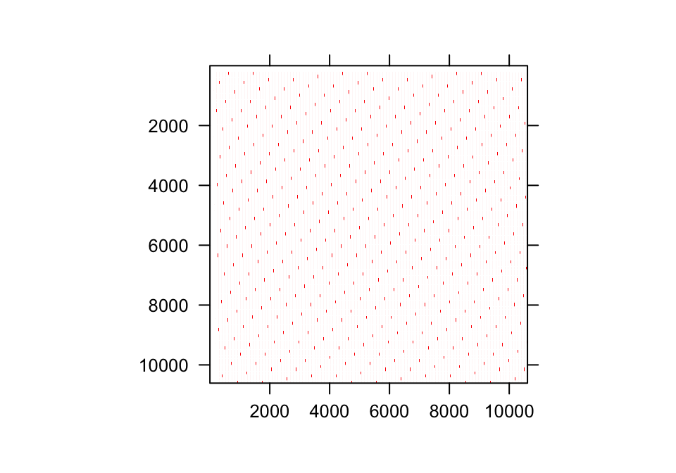
Figure 7.5: Matrix image of the first historical IPM. Red area corresponds to non-zero elements
We can also focus in on just the survival or fecundity transitions, as below. Note that in an ahistorical IPM, we typically expect all fecundity values to be located toward the top of the matrix (figure 7.6), while in a historical MPM they will be distributed across the MPM. Let’s take a look at the ahistorical case.
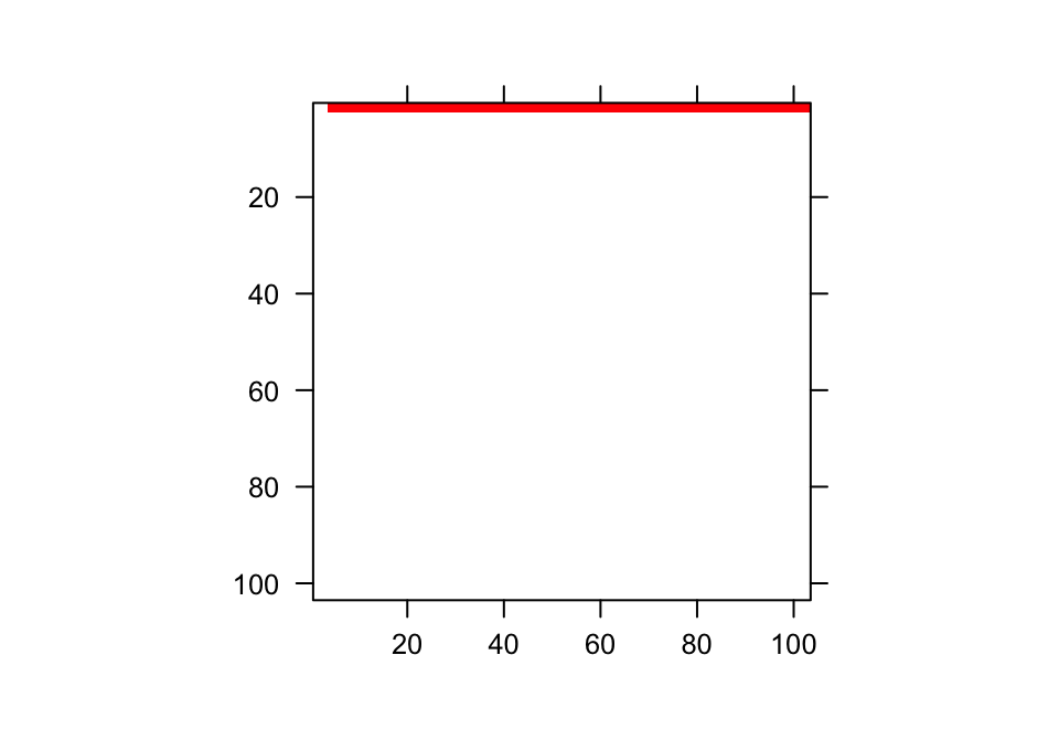
Figure 7.6: Matrix image of the first fecundity matrix in our ahistorical IPM. Red area corresponds to non-zero elements
And now the historical case. Note that you may have to squint to see the fecundity elements, since they are individually dispersed throughout.
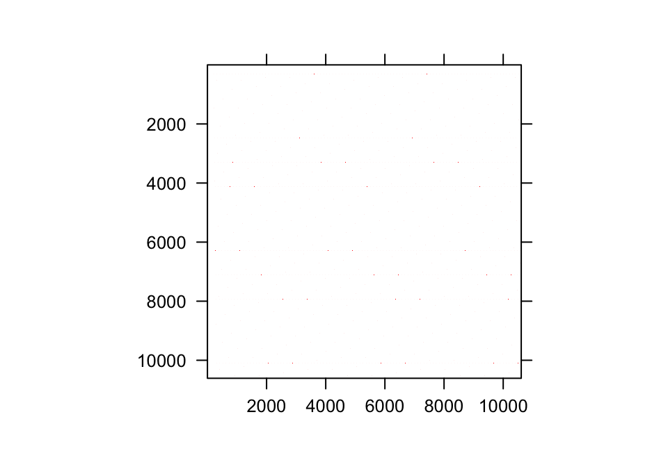
Figure 7.7: Matrix image of the first fecundity matrix in our historical IPM. Red area corresponds to non-zero elements
Other approaches to quality control are provided for other aspects of matrix analysis in lefko3.
7.4 Bootstrapping IPMs
IPMs are essentially function-based MPMs, and the correct way to create IPMs of bootstrapped data is exactly the same as for function-based MPMs. So, first we bootstrap the original dataset, then we create the bootstrapped modelsuite, and finally we run the matrix creation function. Let’s see this in action with the ahistorical IPM. We’ll start by bootstrapping the dataset.
lathvertipm_boot <- bootstrap3(lathvertipm, reps = 10)

summary_hfv(lathvertipm_boot)
>
> This hfvlist object contains 10 hfvdata demographic data frames.
> Each data frame contains an average of 2538.2 rows, 54 variables, 1 population,
> 1 patch, 665.1 individuals, and 3 time steps.
>
> Across all data frames, there are 1 unique population, 1 unique patch, 1053 unique individuals, and 3 unique time steps.
Now we’ll create the bootstrapped modelsuites corresponding to the dataset replicates.
lathmodels2ipm_boot <- modelsearch(lathvertipm_boot, historical = FALSE,
  approach = "mixed", suite = "size", juvestimate = "Sdl",
  vitalrates = c("surv", "obs", "size", "fec"), bestfit = "AICc&k",
  sizedist = "gaussian", fecdist = "negbin", fec.zero = TRUE, indiv = "individ",
  year = "year2", year.as.random = TRUE, juvsize = TRUE,
  show.model.tables = TRUE, quiet = "partial")
Finally, let’s create our bootstrapped MPMs, and run a summary call.
lathmat2ipm_boot <- flefko2(stageframe = lathframeipm, modelsuite = lathmodels2ipm_boot,
  supplement = lathsupp2, data = lathvertipm_boot, reduce = FALSE)

summary(lathmat2ipm_boot)
>
> This lefkoMatList object contains 10 ahistorical lefkoMat objects.
> The average lefkoMat object contains 3 matrices.
>
> This lefkoMatList object covers an average of 1 population, 1 patch, and 3 time steps.
> Each matrix is square with 103 rows and columns, and a total of 10609 elements.
> An average of 30331.7 survival transitions were estimated in each lefkoMat object,
> with an average of 10110.567 per matrix.
> An average of 600 fecundity transitions were estimated in each lefkoMat object,
> with an average of 200 per matrix.
>
> The datasets contain an average total of 670 unique individuals and 2548 unique transitions.
>
> Vital rate modeling quality control:
>
> Survival estimated with an average of 593 individuals and 2248 individual transitions.
> Observation estimated with an average of 548 individuals and 2123 individual transitions.
> Primary size estimated with an average of 540 individuals and 1907 individual transitions.
> Secondary size transition not estimated.
> Tertiary size transition not estimated.
> Reproduction probability not estimated.
> Fecundity estimated with an average of 593 individuals and 2248 individual transitions.
> Juvenile survival estimated with an average of 184 individuals and 288 individual transitions.
> Juvenile observation estimated with an average of 138 individuals and 218 individual transitions.
> Juvenile primary size estimated with an average of 128 individuals and 198 individual transitions.
> Juvenile secondary size transition not estimated.
> Juvenile tertiary size transition not estimated.
> Juvenile reproduction probability not estimated.
> Juvenile maturity transition probability not estimated.
At this point, we may move ahead and analyze the IPMs in the same ways that we might analyze other kinds of MPMs.
7.5 Points to remember
- IPMs assume a continuous distribution for size and integrate vital rates across this size metric. The most common distribution used is the Gaussian distribution. While theoretically different from MPMs, ultimately IPMs are discretized in ways that allow them to be created and analyzed exactly the same way as function-based MPMs.
- Package
lefko3allows the development of even extremely large numbers of size bins across the range of a continuous size metric, using the"ipm"shorthand in thesf_create()function. With only a few lines, a stageframe with hundreds of discretized size bins can be created and used to create an IPM for analysis.
- Care should be taken to ensure that the maximum and minimum limits of the size variable(s) used for classification, together with the resolution of the size bin mesh, do not create size bins that fall outside of the observed range. This may result in IPM eviction, and lead to erroneous inference.
- Quality control tools include the linear model accuracy and R2 / pseudo-R2 output from
modelsearch(), the output fromsummary()calls for IPMs created withflefko2()orflefko3(), and visualization withimage3().
- IPMs may be created from bootstrapped demographic datasets using the same approach used for function-based MPMs.