Chapter 5 Matrix Models II: Function-based MPMs
There is a simple rule here, a rule of legislation, a rule of business, a rule of life: beyond a certain point, complexity is fraud.
Matrix projection models, whether historical or ahistorical, can be categorized as either 1) raw, also called empirical, or 2) function-based, also sometimes called complex IPMs (see chapter 7 for details on the differences). The oldest and most common in the literature is the raw MPM, and chapter 4 discusses that approach in detail. In this chapter, we will cover the function-based approach.
Function-based MPMs are created differently than raw MPMs. Although they can look the same to the untrained eye, and although the matrix elements themselves still represent survival-transition probabilities and fecundity rates, matrix elements are calculated differently. Rather than estimating matrix elements as proportions of individuals moving between stages at consecutive occasions or as products of average offspring production and related recruitment terms from the original dataset, matrix elements in function-based MPMs are estimated using mathematical functions that represent the vital rates or demographic processes underlying the dynamics of the population. These functions are linked together via kernels that treat them typically as conditional rates and probabilities.
How are these vital rate functions estimated? Let’s consider a simple function-based size-classified model. In this model, the survival-transition probability is estimated as the product of the probability that an individual in stage \(j\) at occasion t survives to occasion t+1, and the probability that the same individual becomes stage \(k\) in time t+1 assuming survival to that time. The latter probability is conditional on the first. Thus, we have the following product, where \(\sigma _{j}\) is the survival probability of an individual in stage \(j\) at time t to time t+1, and \(\psi _{kj}\) is the probability of transition from stage \(j\) in time t to stage \(k\) in time t+1 assuming survival to time t+1.
\[\begin{equation} a _{kj} = \sigma _{j} \psi _{kj} \tag{5.1} \end{equation}\]
Continuing with this simple case, fecundity elements assuming a pre-breeding model are given as
\[\begin{equation} a _{kj} = f_{kj} \sigma _{k.} \tag{5.2} \end{equation}\]
and assuming a post-breeding model are given as
\[\begin{equation} a _{kj} = \sigma _{.j} f_{kj} \tag{5.3} \end{equation}\]
where \(f_{kj}\) is the production of stage \(k\) offspring by a reproductive individual in stage \(j\) in time t, \(\sigma _{k.}\) is the survival probability of newborns to age 1 at time t+1 when they are first censused (assuming a pre-breeding model), and \(\sigma _{.j}\) is the survival of the parent from the occasion preceding reproduction to the time of reproduction (assuming a post-breeding model). Note that reproductive stages are defined differently in the post-breeding model than in the pre-breeding model to account for the need to incorporate parental survival in the fecundity transition in the former, but juvenile survival in the latter (see Chapter 2 for further details).
Complexity in the life history model generally increases the number of terms to be multiplied to produce each corresponding element. For example, if we are dealing with an herbaceous plant that undergoes vegetative dormancy, then we might change the survival-transition kernel to two different forms, with the equation used dependent on whether the stage we are transitioning to in time t+1 is dormancy or not. A dormant plant has no aboveground size, and so the equation used for dormancy would be the following instead of equation (5.1), where \(\rho _{.}\) is the probability of sprouting in time t+1 assuming survival from time t and stage \(D\) is the dormant stage.
\[\begin{equation} a _{Dj} = \sigma _{j} (1 - \rho _{.}) \tag{5.4} \end{equation}\]
The probability of transitioning to a non-dormant stage \(k\) is given as
\[\begin{equation} a _{kj} = \sigma _{j} \rho _{.} \psi _{kj} \tag{5.5} \end{equation}\]
where \(\psi _{kj}\) is the transition probability from stage \(j\) in time t to stage \(k\) in time t+1 assuming both survival to time t+1 and sprouting in time t+1. This makes \(\psi _{kj}\) here a little different than \(\psi _{kj}\) in equation (5.1), where we assumed a life history that did not involve the possibility of unobservable life stages.
Size in function-based MPMs is handled using size classes, which often have size bins set to standardized widths. Such widths may be set to 1.0, as might be typical of count variables, but they can also be set narrower or wider. The function-based approach is very flexible, and allows stages and their associated size classes to be cut quite finely by using different vital rate functions on a case-by-case basis. For example, we may wish to create two sets of stages that have the same size classes, but differ in reproductive status. In the herbaceous perennial plant case that we have been working with, such a matrix would be composed of survival-transition probabilities determined by three functions. The first would be given by equation (5.4), for the dormant plant case. The second would be the following equation, corresponding to the transition to non-reproductive stage \(k\), where \(\gamma _{k}\) is the probability of becoming reproductive in time t+1 of an individual in size class \(k\) in that time.
\[\begin{equation} a _{kj} = \sigma _{j} \rho _{.} \psi _{kj} (1 - \gamma _{k}) \tag{5.6} \end{equation}\]
Finally, we have the following equation giving the survival-transition probability to reproductive stage \(k\).
\[\begin{equation} a _{kj} = \sigma _{j} \rho _{.} \psi _{kj} \gamma _{k} \tag{5.7} \end{equation}\]
The functions used in these equations can be developed in several ways. In lefko3, we utilize the linear modeling approach. In this approach, we use hfv-formatted datasets to analyze the main vital rates via either generalized linear models or generalized linear mixed models. The best-fit models are then used as inputs into general functions created for the job, with a great deal of flexibility provided for the assumptions inherent in the system being analyzed. Next, we will describe this approach, but note that linear vital rate models may also be imported (see Chapter 15 for more information).
5.1 Developing vital rate models
Package lefko3 employs two methods to estimate the vital rates used to create function-based MPMs. The main method is automated vital rate modeling. Alternatively, users may create their own vital rate models separately and incorporate them into their MPMs. In lefko3, the function modelsearch() is the main tool provided to estimate vital rate functions via the former method. It also allows users to explore whether history influences component vital rates within a rigorous statistical framework. The results can be used not only to decide whether a historical MPM is justified, but also to develop function-based hMPMs and ahMPMs, including age-by-stage MPMs and even integral projection models (IPMs). Package lefko3 can estimate linear models for up to 14 different vital rates:
- Survival probability - This is the probability of surviving from occasion t to occasion t+1, given that the individual is in stage \(j\) in occasion t (and, if historical, in stage \(l\) in occasion t-1). This parameter may be modeled as a function of up to three size metrics, reproductive status, patch, year, age, and individual identity, and density and a number of annual, individual, or environmental covariates in occasions t and t-1. This parameter is required in all function-based matrices.
- Observation probability - This is the probability of observation in occasion t+1 of an individual in stage \(k\) given survival from occasion t to occasion t+1. This parameter is only used when at least one stage is technically not observable. For example, some plants are capable of vegetative dormancy, in which case they are alive but do not necessarily sprout in all years. In these cases, the probability of sprouting may be estimated as the observation probability. Note that this probability does not refer to observer effort, and so should only be used to differentiate completely unobservable stages where the observation status refers to an important biological phenomenon, such as when individuals may be alive but have a size of zero. This parameter may be modeled as a function of up to three size metrics, reproductive status, patch, year, age, and individual identity, and density and a number of annual, individual, or environmental covariates in occasions t and t-1.
- Primary size transition probability - This is the probability of becoming size \(k\) in occasion t+1 assuming survival from occasion t to occasion t+1 and observation in that time. If multiple size metrics are used, then this refers only to the first of these, which we may refer to as the primary size variable. This parameter may be modeled as a function of up to three size metrics, reproductive status, patch, year, age, and individual identity, and density and a number of annual, individual, or environmental covariates in occasions t and t-1. This parameter is required in all function-based size-classified matrices.
- Secondary size transition probability - This is the probability of becoming size \(k\) in occasion t+1 assuming survival from occasion t to occasion t+1 and observation in that time, within a second size metric used for classification in addition to the primary metric. This parameter may be modeled as a function of up to three size metrics, reproductive status, patch, year, age, and individual identity, and density and a number of annual, individual, or environmental covariates in occasions t and t-1.
- Tertiary size transition probability - This is the probability of becoming size \(k\) in occasion t+1 assuming survival from occasion t to occasion t+1 and observation in that time, within a third size metric used for classification in addition to the primary and secondary metrics. This parameter may be modeled as a function of up to three size metrics, reproductive status, patch, year, age, and individual identity, and density and a number of annual, individual, or environmental covariates in occasions t and t-1.
- Reproduction probability - This is the probability of becoming reproductive in occasion t+1 given survival from occasion t to occasion t+1, and observation in that time. This vital rate should only be used only if the life history model separates breeding from non-breeding mature stages having the same sizes. If all adult stages are potentially reproductive and no separation of reproducing from non-reproducing adults is required by the life history model, then this parameter should not be estimated. This parameter may be modeled as a function of up to three size metrics, reproductive status, patch, year, age, and individual identity, and density and a number of annual, individual, or environmental covariates in occasions t and t-1.
- Fecundity rate - This refers to the rate of production of new individuals into juvenile stages in time t+1 as offspring from reproduction events happening in time t. Under the default setting, this is the rate of successful production of offspring in occasion t by individuals alive, observable, and reproductive in that time, and, if assuming a pre-breeding model and sufficient information is provided in the dataset, the survival of those offspring into occasion t+1 in whatever juvenile class is possible. Thus, the fecundity rate of seed-producing plants might be split into seedlings, which are plants that germinated within a year of seed production, and dormant seeds. Alternatively, it may be given only as produced fruits or seeds, with the survival and germination of seeds provided elsewhere in the MPM development process, such as within a supplement table. An additional setting allows fecundity rate to be estimated using data provided for occasion t+1 instead of occasion t. This parameter may be modeled as a function of up to three size metrics, reproductive status, patch, year, age, and individual identity, and density and a number of annual, individual, or environmental covariates in occasions t and t-1.
- Juvenile survival probability - This is the probability of surviving from juvenile stage \(j\) in occasion t to occasion t+1. It is used only when the user wishes to model vital rates for a single size-unclassified juvenile period separately from adults. This parameter may be modeled as a function of up to three size metrics, patch, year, and individual identity, and density and a number of annual, individual, or environmental covariates in occasions t and t-1.
- Juvenile observation probability - This is the probability of observation in occasion t+1 of an individual in juvenile or mature stage \(j\) in occasion t given survival from occasion t to occasion t+1. It is used only when the user wishes to model vital rates for a single size-unclassified juvenile period separately from adults. This parameter may be modeled as a function of up to three size metrics, patch, year, and individual identity, and density and a number of annual, individual, or environmental covariates in occasions t and t-1.
- Juvenile primary size transition probability - This is the probability of becoming stage \(k\) in occasion t+1 assuming survival from juvenile stage \(j\) in occasion t to occasion t+1 and observation in that time. It is used only when the user wishes to model vital rates for a single size-unclassified juvenile period separately from adults. This parameter may be modeled as a function of up to three size metrics, patch, year, and individual identity, and density and a number of annual, individual, or environmental covariates in occasions t and t-1.
- Juvenile secondary size transition probability - This is the probability of becoming stage \(k\) in occasion t+1 assuming survival from juvenile stage \(j\) in occasion t to occasion t+1 and observation in that time, in a secondary size metric in addition to the primary size metric. It is used only when the user wishes to model vital rates for a single size-unclassified juvenile period separately from adults. This parameter may be modeled as a function of up to three size metrics, patch, year, and individual identity, and density and a number of annual, individual, or environmental covariates in occasions t and t-1.
- Juvenile tertiary size transition probability - This is the probability of becoming stage \(k\) in occasion t+1 assuming survival from juvenile stage \(j\) in occasion t to occasion t+1 and observation in that time, in a tertiary size metric in addition to the primary and secondary size metrics. It is used only when the user wishes to model vital rates for a single size-unclassified juvenile period separately from adults. This parameter may be modeled as a function of up to three size metrics, patch, year, and individual identity, and density and a number of annual, individual, or environmental covariates in occasions t and t-1.
- Juvenile reproduction probability - This is the probability of reproducing in mature stage \(k\) in occasion t+1 given survival from juvenile stage \(j\) in occasion t to occasion t+1, and observation in that time. It is used only when the user wishes to model vital rates for a single size-unclassified juvenile period separately from adults. This parameter may be modeled as a function of up to three size metrics, patch, year, and individual identity, and density and a number of annual, individual, or environmental covariates in occasions t and t-1.
- Juvenile maturity probability - This is the probability of becoming mature in occasion t+1 given survival from juvenile stage \(j\) in occasion t to occasion t+1. It is used only when the user wishes to model vital rates for a single size-unclassified juvenile period separately from adults. This parameter may be modeled as a function of up to three size metrics, patch, year, and individual identity, and density and a number of annual, individual, or environmental covariates in occasions t and t-1. Note that this parameter denotes transition to maturity.
Of these fourteen vital rates, most users will estimate at least parameters (1) survival probability, (3) primary size transition probability, and (7) fecundity rate. These three are the default set for function modelsearch(). Parameters (2) observation probability and (6) reproduction probability may be used when some stages are included that are completely unobservable (and so do not have any size), or that are mature but non-reproductive, respectively. Parameters (4) secondary size transition and (5) tertiary size transition should only be used when size classification involves more than one size variable. Parameters (8) through (14) should only be added if the dataset contains juvenile individuals transitioning to maturity, and these juveniles live within a single juvenile stage for a short time before transitioning to maturity, or before transitioning to a stage that is size-classified in the same manner as adult stages are. If juveniles can be classified by size similarly to adults (or at least on the same scale), then only vital rates (1) through (7) should be used and stage groups can be used with supplement tables to disallow transitions back to juvenile stages. If multiple juvenile stages exist on a different size classification system than adults, then stage groups may also be included as categorical variables in linear vital rate modeling in rates (1) through (7) to stratify vital rate models properly.
5.1.1 Options in modeling vital rates with modelsearch()
Function modelsearch() handles the entire modeling process using an exhaustive model building process combined with information theoretical model selection using model AICc and the number of estimated parameters in each model. It first develops global models, and then develops all nested models via exhaustive model building. Finally, it determines and selects the best-fit models. Users may provide this function with information about the following:
- Individual history - Are the matrices to be built historical or ahistorical? If the former, then the state of the individual in occasion t-1 will be included in modeling.
- Modeling approach - Should the models be estimated as generalized linear models (GLMs) or as generalized linear mixed models (GLMMs, the default)? While most function-based matrix models in the literature are estimated via the former, the latter approach can account for repeated observations of the same individual by including individual identity as a random factor. Mixed models also allow time and patch to be treated as random variables, which allows for broader and more theoretically sound inference.
- Suite of factors - Should both size and reproductive status be tested as causal factors? Should two-way interactions be included? Should only the y-intercept be estimated? Should age be tested exclusively?
- Suite of vital rates - Which adult demographic parameters should be estimated? The defaults are (1) survival, (3) primary size, and (7) fecundity. Should (2) observation status, (4) secondary size, (5) tertiary size, or (6) reproductive status also be modeled?
- Juvenile vital rate estimation - Should juvenile parameters (8) through (14) also be modeled?
- Best-fit criterion - If a model with fewer parameters exists with \(\Delta AICc \leq 2.0\), then should this model be used as the best-fit model (the default), or should the model with the minimum \(AICc\) always be chosen?
- Size distribution - Should size be modeled as a continuous variable under a Gaussian or a gamma distribution, or as a count variable under either a Poisson or negative binomial distribution? If as a count variable, then should the distribution be zero-inflated to account for excess zeros, zero-truncated to account for a lack of zeros, or left unaltered? Similar settings exist for secondary and tertiary size variables, if used.
- Fecundity distribution - Should fecundity be modeled as a continuous variable under a Gaussian or a gamma distribution, or as a count variable under either a Poisson or negative binomial distribution? If a count variable, then should the distribution be zero-inflated to account for excess zeros, zero-truncated to account for a lack of zeros, or left unaltered?
- Timing of fecundity - Although fecundity refers to the production of offspring in stages alive in time t+1, fecundity may be measured differently in different studies. Function
modelsearch()assumes that linear models of fecundity use a metric counted or measured in occasion t as the response. This applies well with most herbaceous plant datasets, where flowers or seeds produced in one year might be the proper fecundity proxy measured. However, users not wishing to follow this default behavior can use thefectimeoption to stipulate a fecundity metric measured in occasion t+1. - Age - Is an age-classified (Leslie) or age-by-stage MPM the main goal?
- Annual covariates - Should the effects of annual covariates on vital rates be tested? If so, should they be treated as fixed, quantitative terms or as random, categorical terms? Do they vary by population / patch, or only by time?
- Individual covariates and environmental state variables - Should the effects of any individual or environmental covariates on vital rates also be tested? If so, should they be treated as fixed, quantitative terms or as random, categorical terms? Do they vary by individual, by population / patch, or only by time?
- Density - Should spatial density be included as a factor in modeling? Note that this refers to local, spatial density with respect to each individual, rather than to the aggregate population size.
- Stage groups - If stage groups are noted in the stageframe, then should they also be used as fixed, independent categorical predictors in modeling?
- Censoring - Should data points marked as questionable be used in or excluded from modeling?
- Variable names - The names of all relevant variables in the dataset need to be specified. Note that the default behavior assumes the default variable names produced via functions
historicalize3()orverticalize3(). - Global model only - Should a full exhaustive model building and selection exercise be performed (the default), or should only the global model be built and parameterized?
- Accuracy - Should the accuracy of binomial models, and simple R2 or pseudo-R2 of size and fecundity models be evaluated?
- Keep data subsets - Function
modelsearch()subsets the data for each vital rate modeling exercise. Should those datasets be kept in the output?
Once all decisions have been made and associated input terms have been provided, modelsearch() goes to work. The result is a lefkoMod object, which is a list in which the first 14 elements are the best-fit models developed for each vital rate. These are followed by an equivalent number of elements showing the full model tables developed and tested, followed by a table of parameter names (object paramnames), an element detailing the best-fit criterion used (object criterion), and ending on quality control data showing the number of individuals and the number of unique transitions used in the estimation of each model, and the accuracy or simple R2 of each model (object qc). The user may also output data subsets used to generate each vital rate model, within a list held as a single element of the top-level list. Depending on user choices, linear modeling is handled through the lm() and glm() functions in the stats package, the lmer() and glmer() functions in lme4, the glmmTMB() function in package glmmTMB, the glm.nb() function in package MASS, the vglm() function in package VGAM, or the zeroinfl() function in package pscl. Exhaustive model building proceeds through the dredge() function in package MuMIn (Bartoń 2014). Model selection is handled through assessment of \(AICc\) and the degrees of freedom (\(k\)) estimated per model by default (see 6. Best-fit criterion above).
If modelsearch() is set for historical analysis (historical = TRUE, the default), then the decision of whether to develop a historical MPM can be made on the basis of whether any best-fit vital rate model includes size or reproductive status in occasion t-1. If at least one vital rate does, then a historical MPM is justified. Otherwise, it is not. Regardless, the output can be used to create a function-based MPM in the next step.
5.2 Assessing vital rates in Cypripedium candidum
Let’s now work on the Cypripedium candidum case study. We introduced the model and code for our stageframe and supplements in Chapter 2. However, as it has likely been a while since we have viewed that chapter, let’s take a look again at the life history model that we will use (5.1; note that this is the same as figure 2.3).
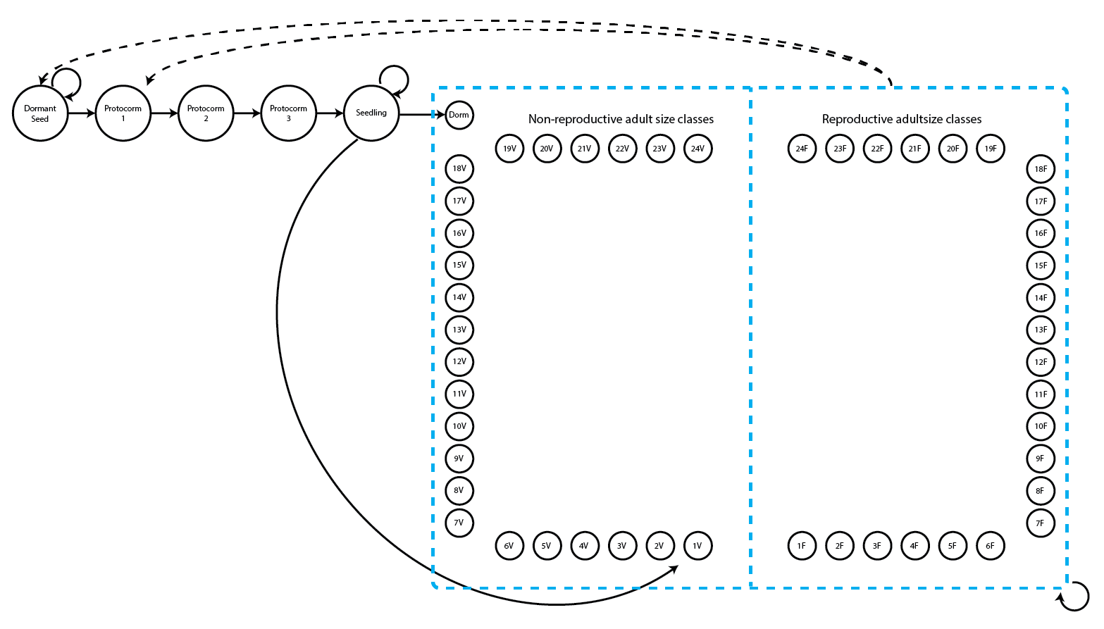
This is a fairly large life history model with two adult life stages for each number of sprouts - a reproductive stage that flowers and a non-reproductive stage that does not flower. Let’s load the raw dataset first. Then we will set up our stageframe and standardize the data into a historically formatted vertical (hfv) data frame.
data(cypdata)

stagevector <- c("SD", "P1", "P2", "P3", "SL", "Dorm", "1V", "2V", "3V", "4V",
  "5V", "6V", "7V", "8V", "9V", "10V", "11V", "12V", "13V", "14V", "15V", "16V",
  "17V", "18V", "19V", "20V", "21V", "22V", "23V", "24V", "1F", "2F", "3F",
  "4F", "5F", "6F", "7F", "8F", "9F", "10F", "11F", "12F", "13F", "14F", "15F",
  "16F", "17F", "18F", "19F", "20F", "21F", "22F", "23F", "24F")
indataset <- c(0, 0, 0, 0, 0, rep(1, 49))
sizevector <- c(0, 0, 0, 0, 0, seq(from = 0, t = 24), seq(from = 1, to = 24))
repvector <- c(0, 0, 0, 0, 0, rep(0, 25), rep(1, 24))
obsvector <- c(0, 0, 0, 0, 0, 0, rep(1, 48))
matvector <- c(0, 0, 0, 0, 0, rep(1, 49))
immvector <- c(0, 1, 1, 1, 1, rep(0, 49))
propvector <- c(1, rep(0, 53))
comments <- c("Dormant seed", "Yr1 protocorm", "Yr2 protocorm", "Yr3 protocorm",
  "Seedling", "Veg dorm", "Veg adult 1 stem", "Veg adult 2 stems",
  "Veg adult 3 stems", "Veg adult 4 stems", "Veg adult 5 stems",
  "Veg adult 6 stems", "Veg adult 7 stems", "Veg adult 8 stems",
  "Veg adult 9 stems", "Veg adult 10 stems", "Veg adult 11 stems",
  "Veg adult 12 stems", "Veg adult 13 stems", "Veg adult 14 stems",
  "Veg adult 15 stems", "Veg adult 16 stems", "Veg adult 17 stems",
  "Veg adult 18 stems", "Veg adult 19 stems", "Veg adult 20 stems",
  "Veg adult 21 stems", "Veg adult 22 stems", "Veg adult 23 stems",
  "Veg adult 24 stems", "Flo adult 1 stem", "Flo adult 2 stems",
  "Flo adult 3 stems", "Flo adult 4 stems", "Flo adult 5 stems",
  "Flo adult 6 stems", "Flo adult 7 stems", "Flo adult 8 stems",
  "Flo adult 9 stems", "Flo adult 10 stems", "Flo adult 11 stems",
  "Flo adult 12 stems", "Flo adult 13 stems", "Flo adult 14 stems",
  "Flo adult 15 stems", "Flo adult 16 stems", "Flo adult 17 stems",
  "Flo adult 18 stems", "Flo adult 19 stems", "Flo adult 20 stems",
  "Flo adult 21 stems", "Flo adult 22 stems", "Flo adult 23 stems",
  "Flo adult 24 stems")

cypframe_fb <- sf_create(sizes = sizevector, stagenames = stagevector,
  repstatus = repvector, obsstatus = obsvector, matstatus = matvector,
  propstatus = propvector, immstatus = immvector, indataset = indataset,
  comments = comments)

cypfb_v1 <- verticalize3(data = cypdata, noyears = 6, firstyear = 2004,
  patchidcol = "patch", individcol = "plantid", blocksize = 4,
  sizeacol = "Inf2.04", sizebcol = "Inf.04", sizeccol = "Veg.04",
  repstracol = "Inf.04", repstrbcol = "Inf2.04", fecacol = "Pod.04",
  stageassign = cypframe_fb, stagesize = "sizeadded", NAas0 = TRUE,
  age_offset = 4)
Now we will load the supplement tables that we will use for the ahistorical and historical MPMs. Note that these are slightly different from the previous chapter (chapter 4), because of the different life history model that we are using.
seeds_per_fruit <- 5000
sl_mult <- 0.7

cypsupp2_fb <- supplemental(stage3 = c("SD", "P1", "P2", "P3", "SL", "SL",
    "Dorm", "1V", "2V", "3V", "SD", "P1"),
  stage2 = c("SD", "SD", "P1", "P2", "P3", "SL", "SL", "SL", "SL", "SL", "rep",
    "rep"),
  eststage3 = c(NA, NA, NA, NA, NA, NA, "Dorm", "1V", "2V", "3V", NA, NA),
  eststage2 = c(NA, NA, NA, NA, NA, NA, "Dorm", "Dorm", "Dorm", "Dorm", NA, NA),
  givenrate = c(0.08, 0.1, 0.1, 0.1, 0.05, 0.05, NA, NA, NA, NA, NA, NA),
  multiplier = c(NA, NA, NA, NA, NA, NA, sl_mult, sl_mult, sl_mult, sl_mult,
    0.5 * seeds_per_fruit, 0.5 * seeds_per_fruit),
  type = c("S", "S", "S", "S", "S", "S", "S", "S", "S", "S", "R", "R"),
  stageframe = cypframe_fb, historical = FALSE)
> Warning: NA values in argument multiplier will be treated as 1 values.

cypsupp3_fb <- supplemental(stage3 = c("SD", "SD", "P1", "P1", "P2", "P3",
    "SL", "SL", "SL", "Dorm", "1V", "2V", "3V", "Dorm", "1V", "2V", "3V", "mat",
    "mat", "mat", "mat", "SD", "P1"),
  stage2 = c("SD", "SD", "SD", "SD", "P1", "P2", "P3", "SL", "SL", "SL", "SL",
    "SL", "SL", "SL", "SL", "SL", "SL", "Dorm", "1V", "2V", "3V", "rep", "rep"),
  stage1 = c("SD", "rep", "SD", "rep", "SD", "P1", "P2", "P3", "SL", "P3", "P3",
    "P3", "P3", "SL", "SL", "SL", "SL", "SL", "SL", "SL", "SL", "mat", "mat"),
  eststage3 = c(NA, NA, NA, NA, NA, NA, NA, NA, NA, "Dorm", "1V", "2V", "3V",
    "Dorm", "1V", "2V", "3V", "mat", "mat", "mat", "mat", NA, NA),
  eststage2 = c(NA, NA, NA, NA, NA, NA, NA, NA, NA, "Dorm", "Dorm", "Dorm",
    "Dorm", "Dorm", "Dorm", "Dorm", "Dorm", "Dorm", "1V", "2V", "3V", NA, NA),
  eststage1 = c(NA, NA, NA, NA, NA, NA, NA, NA, NA, "Dorm", "Dorm", "Dorm",
    "Dorm", "Dorm", "Dorm", "Dorm", "Dorm", "1V", "1V", "1V", "1V", NA, NA),
  givenrate = c(0.08, 0.08, 0.1, 0.1, 0.1, 0.1, 0.1, 0.05, 0.05, NA, NA, NA, NA,
    NA, NA, NA, NA, NA, NA, NA, NA, NA, NA),
  multiplier = c(NA, NA, NA, NA, NA, NA, NA, NA, NA, sl_mult, sl_mult,
    sl_mult, sl_mult, sl_mult, sl_mult, sl_mult, sl_mult, 1, 1, 1, 1,
    0.5 * seeds_per_fruit, 0.5 * seeds_per_fruit),
  type = c("S", "S", "S", "S", "S", "S", "S", "S", "S", "S", "S", "S", "S", "S",
    "S", "S", "S", "S", "S", "S", "S", "R", "R"),
  type_t12 = c("S", "F", "S", "F", "S", "S", "S", "S", "S", "S", "S", "S", "S",
    "S", "S", "S", "S", "S", "S", "S", "S", "S", "S"),
  stageframe = cypframe_fb, historical = TRUE)
> Warning: NA values in argument multiplier will be treated as 1 values.
Before we can develop our vital rate models, we need to determine the proper distributions for size and fecundity. As a reminder, size in the Cypripedium dataset is given as a series of numbers of sprouts, and our proxy for size can be either the number of flowers or the number of fruits produced by an individual. So, size and fecundity in this dataset are all non-negative integers, or count variables. Count variables generally break the assumptions of a Gaussian distribution because the mean and variance are strongly related, possible values are discrete, and distributions are often dramatically skewed. Additionally, because we have absorbed individuals with a size of zero into the dormant stage, there are no zeros left for the size model and so we will need a zero-truncated distribution. Fecundity, in contrast, is a count variable that includes zeros and so we should test whether we need a zero-inflated model.
Package lefko3 includes a function that can help in determining which distributions to use, as well as in assessing the quality of the data with respect to the linear models that we wish to develop: hfv_qc(). Let’s try this function out. Note that we need to specify which vital rate models we will be modeling (the vitalrates field below), because the data frame that we will input will be subset according to this decision. We also need to enter the names of the variables we are using, here in particular for size, since we are not using the default variables. In fact, we can load the function with exactly the same input that we are considering using in function modelsearch(), just to simplify life.
hfv_qc(cypfb_v1, vitalrates = c("surv", "obs", "size", "repst", "fec"),
  patch = "patchid", size = c("size3added", "size2added", "size1added"))
> Survival:
>
>   Data subset has 58 variables and 320 transitions.
>
>   Variable alive3 has 0 missing values.
>   Variable alive3 is a binomial variable.
>
>   Numbers of categories in data subset in possible random variables:
>   indiv id: 74   (singleton categories: 6)
>   year2: 5   (singleton categories: 0)
>   patch: 3   (singleton categories: 0)
>
> Observation status:
>
>   Data subset has 58 variables and 303 transitions.
>
>   Variable obsstatus3 has 0 missing values.
>   Variable obsstatus3 is a binomial variable.
>
>   Numbers of categories in data subset in possible random variables:
>   indiv id: 70   (singleton categories: 6)
>   year2: 5   (singleton categories: 0)
>   patch: 3   (singleton categories: 0)
>
> Primary size:
>
>   Data subset has 58 variables and 288 transitions.
>
>   Variable size3added has 0 missing values.
>   Variable size3added appears to be an integer variable.
>
>   Variable size3added is fully positive, lacking even 0s.
>
>   Overdispersion test:
>     Mean size3added is 3.653
>     The variance in size3added is 13.41
>     The probability of this dispersion level by chance assuming that
>     the true mean size3added = variance in size3added,
>     and an alternative hypothesis of overdispersion, is 3.721e-138
>     Variable size3added is significantly overdispersed.
>
>   Zero-inflation and truncation tests:
>     Mean lambda in size3added is 0.02592
>     The actual number of 0s in size3added is 0
>     The expected number of 0s in size3added under the null hypothesis is 7.465
>     The probability of this deviation in 0s from expectation by chance is 0.9964
>     Variable size3added is not significantly zero-inflated.
>
>     Variable size3added does not include 0s, suggesting that a zero-truncated distribution may be warranted.
>
>   Numbers of categories in data subset in possible random variables:
>   indiv id: 70   (singleton categories: 6)
>   year2: 5   (singleton categories: 0)
>   patch: 3   (singleton categories: 0)
>
> Reproductive status:
>
>   Data subset has 58 variables and 288 transitions.
>
>   Variable repstatus3 has 0 missing values.
>   Variable repstatus3 is a binomial variable.
>
>   Numbers of categories in data subset in possible random variables:
>   indiv id: 70   (singleton categories: 6)
>   year2: 5   (singleton categories: 0)
>   patch: 3   (singleton categories: 0)
>
> Fecundity:
>
>   Data subset has 58 variables and 118 transitions.
>
>   Variable feca2 has 0 missing values.
>   Variable feca2 appears to be an integer variable.
>
>   Variable feca2 is fully non-negative.
>
>   Overdispersion test:
>     Mean feca2 is 0.7881
>     The variance in feca2 is 1.536
>     The probability of this dispersion level by chance assuming that
>     the true mean feca2 = variance in feca2,
>     and an alternative hypothesis of overdispersion, is 0.1193
>     Dispersion level in feca2 matches expectation.
>
>   Zero-inflation and truncation tests:
>     Mean lambda in feca2 is 0.4547
>     The actual number of 0s in feca2 is 68
>     The expected number of 0s in feca2 under the null hypothesis is 53.65
>     The probability of this deviation in 0s from expectation by chance is 5.904e-06
>     Variable feca2 is significantly zero-inflated.
>
>   Numbers of categories in data subset in possible random variables:
>   indiv id: 51   (singleton categories: 21)
>   year2: 5   (singleton categories: 0)
>   patch: 3   (singleton categories: 0)
The results show that size is significantly overdispersed and zero-truncated. This means that we cannot use the Poisson distribution, and should instead use the zero-truncated negative binomial distribution. Fecundity is not significantly overdispersed, but it is significantly zero-inflated, so we will require a zero-inflated Poisson distribution. Looking over the other variables, we see that they match the binomial distribution (required for probabilities), and we also see the changing sample size used for the different data subsets that will be used to conduct the linear modeling. The number of categories associated with possible random terms is also much lower than the number of data points in each subset, so the overall quality of the data looks appropriate for mixed modeling.
5.3 Setting up function modelsearch()
Next, we will create a full suite of vital rate models using function modelsearch(). Before proceeding, we need to decide on the linear model building strategy, the correct vital rates to model, the proper statistical distributions for estimated vital rates, the proper parameterization for each vital rate, and the strategy to determine the best-fit models.
First, we must determine the model building strategy. In most cases, the best procedure will be through mixed linear models in which monitoring occasion and individual identity are random terms. We will set monitoring occasion as random because we wish to make inferences for the population as a whole and do not wish to restrict ourselves to inference only for the years monitored (i.e. our distribution of monitoring occasions sampled is itself assumed to be a sample of the population in time). We will set individual identity as random because many or most of the individuals that we have sampled to produce our dataset yield multiple observation data points across time. Thus, we will set approach = "mixed". To make sure that time and individual identity are treated as random, we will set the proper variable names for indiv and year, corresponding to individual identity (individ by default), and to occasion t (year2 by default). The year.as.random option is set to TRUE by default. Setting year.as.random to FALSE would make time a fixed categorical variable in all cases. The patch.as.random option functions similarly with respect to patches / subpopulations.
The mixed modeling approach is usually preferable to the GLM approach because of its treatment of repeat samples. Indeed, treating each transition as independent of every other leads to pseudoreplication if transitions can come from the same individual. Mixed modeling deals with this problem by treating the individual as a random factor. However, the GLM approach is faster and has greater statistical power. Users of package lefko3 wishing to use a standard generalized linear modeling strategy should set approach = "glm". In this case, individual identity is not used, time is a fixed categorical factor (as is patch, if used), and all observed transitions are treated as independent.
Next, we must determine which vital rates to model. The default settings for modelsearch() estimate 1) survival probability, 3) primary size distribution, and 7) fecundity, which are the minimum three vital rates required for a full MPM. Observation probability (option obs in vitalrates) should only be included when a life history stage or size exists that cannot be observed. For example, in the case of a plant with vegetative dormancy, the observation probability can be thought of as the sprouting probability, which is a biologically meaningful vital rate (Shefferson et al. 2001). Further, reproduction status (option repst in vitalrates) should only be modeled if size classification needs to be stratified by the ability to reproduce, as when some individuals with no fecundity occur within stages that also include individuals producing offspring. Since Cypripedium candidum is capable of long bouts of vegetative dormancy, since we wish to stratify the population into reproductive and non-reproductive stages of the same size classes, and since we have no data derived from juvenile individuals, we will set vitalrates = c("surv", "obs", "size", "repst", "fec") and we will not set juvestimate and juvsize.
Third, we need to set the proper statistical distribution for each parameter. Survival probability, observation probability, reproductive status, and maturity status are all modeled as binomial variables, and this cannot be changed. In the case of this population of Cypripedium candidum, size was measured as the number of stems and so is a count variable. Likewise, fecundity is estimated as the number of fruits produced per plant, and so is also a count variable. We have already performed tests for overdispersion and zero-inflation, and we are also aware that size in observed stages cannot be zero, requiring zero-truncation in that parameter. So we will set size to the zero-truncated negative binomial distribution, and fecundity to the zero-inflated Poisson distribution.
Fourth, we need the proper model parameterizations for each vital rate, using the suite option. The default, suite = "main", under the mixed model setting (approach = "mixed") starts with the estimation of global models that include size and reproductive status in occasions t and t-1 as fixed factors, with individual identity and time in occasion t (year t) set as random categorical terms. Setting suite = "full" will yield global models that also include all two-way interactions among size and reproductive status terms. If the population is not stratified by reproductive status, then suite = "size" will eliminate reproductive status terms and use all others in the global model. If size is not important, then suite = "rep" will eliminate size but keep reproductive status and all other terms. Finally, suite = "cons" will result in a global model in which neither reproductive status nor size are considered. Other terms can be specified, including individual or annual covariates, density, and age. The interactions argument allows two-way interactions among these other terms, and with the core size and reproductive status terms (interactions = FALSE by default).
Finally, we should determine the proper strategy for the determination of the best-fit model. Model building proceeds through the dredge() function in package MuMIn (Bartoń 2014), and each model has an associated AICc value. The default setting in lefko3 (bestfit = "AICc&k") will compare all models within 2.0 AICc units of the model with \(\Delta AICc = 0\), and choose the one with the lowest degrees of freedom. This approach is generally better than the alternative, which simply uses the model with \(\Delta AICc = 0\) (bestfit = "AICc"), as all models within 2.0 AICc units of that model are equally parsimonious and so fewer degrees of freedom result from fewer parameters estimated (Burnham & Anderson 2002).
In the model building exercise below, we will use the suite = "main" option to run all main effects only. Normally we would set suite = "full" and interactions = TRUE, but running all effects including their two-way interactions will likely tie up our computers for a little too long for this tutorial. To keep tabs on what is going on, we will set quiet = "partial", which will yield messages showing where the modeling is currently running as it goes. While this runs, feel free to make yourself a coffee or a cappuccino, or perhaps something stronger (no judgement here…).
cypmodels3p <- modelsearch(cypfb_v1, historical = TRUE, approach = "mixed",
  vitalrates = c("surv", "obs", "size", "repst", "fec"), patch = "patchid",
  sizedist = "negbin", size.trunc = TRUE, fecdist = "poisson", fec.zero = TRUE,
  suite = "main", size = c("size3added", "size2added", "size1added"),
  quiet = "partial")
Once done, we will summarize the output with the summary() function.
summary(cypmodels3p)
> This LefkoMod object includes 5 linear models.
> Best-fit model criterion used: aicc&k
>
>
>
> Survival model:
> Generalized linear mixed model fit by maximum likelihood (Laplace
>   Approximation) [glmerMod]
>  Family: binomial  ( logit )
> Formula: alive3 ~ size2added + (1 | year2) + (1 | patchid) + (1 | individ)
>    Data: surv.data
>       AIC       BIC    logLik -2*log(L)  df.resid
>  130.1321  148.9737  -60.0660  120.1321       315
> Random effects:
>  Groups  Name        Std.Dev.
>  individ (Intercept) 1.199e+00
>  year2   (Intercept) 5.117e-05
>  patchid (Intercept) 1.172e-05
> Number of obs: 320, groups:  individ, 74; year2, 5; patchid, 3
> Fixed Effects:
> (Intercept)   size2added
>      2.0356       0.6343
> optimizer (Nelder_Mead) convergence code: 0 (OK) ; 0 optimizer warnings; 1 lme4 warnings
>
>
>
> Observation model:
> Generalized linear mixed model fit by maximum likelihood (Laplace
>   Approximation) [glmerMod]
>  Family: binomial  ( logit )
> Formula: obsstatus3 ~ size2added + (1 | year2) + (1 | patchid) + (1 |
>     individ)
>    Data: obs.data
>       AIC       BIC    logLik -2*log(L)  df.resid
>  120.2567  138.8254  -55.1284  110.2567       298
> Random effects:
>  Groups  Name        Std.Dev.
>  individ (Intercept) 0.0000
>  year2   (Intercept) 0.8776
>  patchid (Intercept) 0.0000
> Number of obs: 303, groups:  individ, 70; year2, 5; patchid, 3
> Fixed Effects:
> (Intercept)   size2added
>      2.4904       0.3134
> optimizer (Nelder_Mead) convergence code: 0 (OK) ; 0 optimizer warnings; 1 lme4 warnings
>
>
>
> Size model:
> Formula:          size3added ~ (1 | year2) + (1 | patchid) + (1 | individ)
> Data: size.data
>       AIC       BIC    logLik -2*log(L)  df.resid
> 1009.9750 1028.2898 -499.9875  999.9750       283
> Random-effects (co)variances:
>
> Conditional model:
>  Groups  Name        Std.Dev.
>  year2   (Intercept) 0.1133
>  patchid (Intercept) 0.2118
>  individ (Intercept) 1.0320
>
> Number of obs: 288 / Conditional model: year2, 5; patchid, 3; individ, 70
>
> Dispersion parameter for truncated_nbinom2 family (): 3.26e+07
>
> Fixed Effects:
>
> Conditional model:
> (Intercept)
>       0.587
>
>
>
> Secondary size model:
> [1] 1
>
>
>
> Tertiary size model:
> [1] 1
>
>
>
> Reproductive status model:
> Generalized linear mixed model fit by maximum likelihood (Laplace
>   Approximation) [glmerMod]
>  Family: binomial  ( logit )
> Formula: repstatus3 ~ repstatus2 + size2added + (1 | year2) + (1 | patchid) +
>     (1 | individ)
>    Data: repst.data
>       AIC       BIC    logLik -2*log(L)  df.resid
>  333.4037  355.3815 -160.7019  321.4037       282
> Random effects:
>  Groups  Name        Std.Dev.
>  individ (Intercept) 0.1776
>  year2   (Intercept) 0.6636
>  patchid (Intercept) 0.3501
> Number of obs: 288, groups:  individ, 70; year2, 5; patchid, 3
> Fixed Effects:
> (Intercept)   repstatus2   size2added
>     -1.3836       1.5543       0.1788
>
>
>
> Fecundity model:
> Formula:
> feca2 ~ size2added + (1 | year2) + (1 | patchid) + (1 | individ)
> Zero inflation:
> ~repstatus1 + size2added + (1 | year2) + (1 | patchid) + (1 |     individ)
> Data: fec.data
>       AIC       BIC    logLik -2*log(L)  df.resid
>  253.3741  283.8516 -115.6870  231.3741       107
> Random-effects (co)variances:
>
> Conditional model:
>  Groups  Name        Std.Dev.
>  year2   (Intercept) 5.615e-01
>  patchid (Intercept) 2.273e-01
>  individ (Intercept) 1.659e-09
>
> Zero-inflation model:
>  Groups  Name        Std.Dev.
>  year2   (Intercept) 5.440e-07
>  patchid (Intercept) 1.019e-12
>  individ (Intercept) 2.201e-04
>
> Number of obs: 118 / Conditional model: year2, 5; patchid, 3; individ, 51 / Zero-inflation model: year2, 5; patchid, 3; individ, 51
>
> Fixed Effects:
>
> Conditional model:
> (Intercept)   size2added
>    -0.56432      0.06241
>
> Zero-inflation model:
> (Intercept)   repstatus1   size2added
>      3.7547       0.3102      -1.6107
>
>
> Juvenile survival model:
> [1] 1
>
>
>
> Juvenile observation model:
> [1] 1
>
>
>
> Juvenile size model:
> [1] 1
>
>
>
> Juvenile secondary size model:
> [1] 1
>
>
>
> Juvenile tertiary size model:
> [1] 1
>
>
>
> Juvenile reproduction model:
> [1] 1
>
>
>
> Juvenile maturity model:
> [1] 1
>
>
>
>
>
> Number of models in survival table: 16
>
> Number of models in observation table: 16
>
> Number of models in size table: 16
>
> Number of models in secondary size table: 1
>
> Number of models in tertiary size table: 1
>
> Number of models in reproduction status table: 16
>
> Number of models in fecundity table: 256
>
> Number of models in juvenile survival table: 1
>
> Number of models in juvenile observation table: 1
>
> Number of models in juvenile size table: 1
>
> Number of models in juvenile secondary size table: 1
>
> Number of models in juvenile tertiary size table: 1
>
> Number of models in juvenile reproduction table: 1
>
> Number of models in juvenile maturity table: 1
>
>
>
>
>
> General model parameter names (column 1), and
> specific names used in these models (column 2):
>                       parameter_names mainparams
> 1                              time t      year2
> 2                          individual    individ
> 3                               patch      patch
> 4                   alive in time t+1      surv3
> 5                observed in time t+1       obs3
> 6                   sizea in time t+1      size3
> 7                   sizeb in time t+1     sizeb3
> 8                   sizec in time t+1     sizec3
> 9     reproductive status in time t+1     repst3
> 10              fecundity in time t+1       fec3
> 11                fecundity in time t       fec2
> 12                    sizea in time t      size2
> 13                  sizea in time t-1      size1
> 14                    sizeb in time t     sizeb2
> 15                  sizeb in time t-1     sizeb1
> 16                    sizec in time t     sizec2
> 17                  sizec in time t-1     sizec1
> 18      reproductive status in time t     repst2
> 19    reproductive status in time t-1     repst1
> 20        maturity status in time t+1     matst3
> 21          maturity status in time t     matst2
> 22                      age in time t        age
> 23                  density in time t    density
> 24   individual covariate a in time t   indcova2
> 25 individual covariate a in time t-1   indcova1
> 26   individual covariate b in time t   indcovb2
> 27 individual covariate b in time t-1   indcovb1
> 28   individual covariate c in time t   indcovc2
> 29 individual covariate c in time t-1   indcovc1
> 30              stage group in time t     group2
> 31            stage group in time t-1     group1
> 32       annual covariate a in time t  annucova2
> 33     annual covariate a in time t-1  annucova1
> 34       annual covariate b in time t  annucovb2
> 35     annual covariate b in time t-1  annucovb1
> 36       annual covariate c in time t  annucovc2
> 37     annual covariate c in time t-1  annucovc1
>
>
>
>
>
> Quality control:
>
> Survival model estimated with 74 individuals and 320 individual transitions.
> Survival model accuracy is 0.947.
> Observation status model estimated with 70 individuals and 303 individual transitions.
> Observation status model accuracy is 0.95.
> Primary size model estimated with 70 individuals and 288 individual transitions.
> Primary size model R-squared is 0.82.
> Secondary size model not estimated.
> Tertiary size model not estimated.
> Reproductive status model estimated with 70 individuals and 288 individual transitions.
> Reproductive status model accuracy is 0.74.
> Fecundity model estimated with 51 individuals and 118 individual transitions.
> Fecundity model R-squared is 0.535.
> Juvenile survival model not estimated.
> Juvenile observation status model not estimated.
> Juvenile primary size model not estimated.
> Juvenile secondary size model not estimated.
> Juvenile tertiary size model not estimated.
> Juvenile reproductive status model not estimated.
> Juvenile maturity status model not estimated.
The above code may take some time to run, depending on how powerful a computer it is run on. It is sufficiently complicated that R might crash if it is run while the user does other things in R or RStudio, so please leave your R or RStudio session alone while it runs. As the function runs, it will likely produce some text related to the modeling. Some of the text is meant to provide guideposts to where the modeling stands. Since the vital rates run in order, the user can get a handle on which vital rate best-fit models are finished and which are still waiting to be developed. Other text relates to notes, warnings, and other messages from the modeling functions used, which are found in other CRAN-based packages. We have set quiet = "partial" to prevent this text from getting very long (quiet = TRUE eliminates just about all of it).
The final object is a class lefkoMod object. This is an S3 object, meaning that it is a list, and it is composed of 31 elements. The first 14 elements are the best-fit models, and are in the formats of the functions used to develop them. The next 14 elements are the MuMIn model tables, showing all of the models tested for each vital rate in order of \(\Delta AICc\) (\(\Delta AICc\) is given as the difference between the \(AICc\) values of the current model and the model with the lowest \(AICc\)). The final three elements are a data frame describing the parameters tested (paramnames), the criterion used for determination of the best-fit model (criterion), and quality control data used in summary() calls (qc).
The summary of this lefkoMod object is quite informative. We start off by seeing the best-fit model chosen for each vital rate. In the case of vital rates that are not estimated, they are set to constants, either 1 or 0. Below that, we see how many models were built and compared for each vital rate. The next section is something of a crib sheet, showing us the names of different parameters used in the modeling. Finally, we see a section on quality control. This last section includes information on the numbers of individuals as well as individual transitions used to parameterize each model, and also shows their accuracy, R2, or pseudo-R2 values. We see very high accuracy in survival and observation status, and a high R2 for primary size, but poorer accuracy in reproduction status and low R2 for fecundity.
Looking over the models, we can also see from the summary that historical terms are only included in the fecundity model. This is likely enough to warrant using a historical model, since accurate estimation of fecundity appears to warrant a historical approach (although the R2 is relatively low, at just over 0.50). Regardless, in order to compare MPMs for educational purposes, we will also create a purely ahistorical model set. We will set quiet = "partial" to see less text output as the function works, but you may remove that option to view the guidepost text. Note that a vital rate model set that includes historical terms should never be used to make an ahistorical MPM.
cypmodels2p <- modelsearch(cypfb_v1, historical = FALSE, approach = "mixed",
  vitalrates = c("surv", "obs", "size", "repst", "fec"), patch = "patchid",
  sizedist = "negbin", size.trunc = TRUE, fecdist = "poisson", fec.zero = TRUE,
  suite = "main", size = c("size3added", "size2added", "size1added"),
  quiet = "partial")
Let’s see a summary of this lefkoMod object.
summary(cypmodels2p)
> This LefkoMod object includes 5 linear models.
> Best-fit model criterion used: aicc&k
>
>
>
> Survival model:
> Generalized linear mixed model fit by maximum likelihood (Laplace
>   Approximation) [glmerMod]
>  Family: binomial  ( logit )
> Formula: alive3 ~ size2added + (1 | year2) + (1 | patchid) + (1 | individ)
>    Data: surv.data
>       AIC       BIC    logLik -2*log(L)  df.resid
>  130.1321  148.9737  -60.0660  120.1321       315
> Random effects:
>  Groups  Name        Std.Dev.
>  individ (Intercept) 1.199e+00
>  year2   (Intercept) 5.117e-05
>  patchid (Intercept) 1.172e-05
> Number of obs: 320, groups:  individ, 74; year2, 5; patchid, 3
> Fixed Effects:
> (Intercept)   size2added
>      2.0356       0.6343
> optimizer (Nelder_Mead) convergence code: 0 (OK) ; 0 optimizer warnings; 1 lme4 warnings
>
>
>
> Observation model:
> Generalized linear mixed model fit by maximum likelihood (Laplace
>   Approximation) [glmerMod]
>  Family: binomial  ( logit )
> Formula: obsstatus3 ~ size2added + (1 | year2) + (1 | patchid) + (1 |
>     individ)
>    Data: obs.data
>       AIC       BIC    logLik -2*log(L)  df.resid
>  120.2567  138.8254  -55.1284  110.2567       298
> Random effects:
>  Groups  Name        Std.Dev.
>  individ (Intercept) 0.0000
>  year2   (Intercept) 0.8776
>  patchid (Intercept) 0.0000
> Number of obs: 303, groups:  individ, 70; year2, 5; patchid, 3
> Fixed Effects:
> (Intercept)   size2added
>      2.4904       0.3134
> optimizer (Nelder_Mead) convergence code: 0 (OK) ; 0 optimizer warnings; 1 lme4 warnings
>
>
>
> Size model:
> Formula:          size3added ~ (1 | year2) + (1 | patchid) + (1 | individ)
> Data: size.data
>       AIC       BIC    logLik -2*log(L)  df.resid
> 1009.9750 1028.2898 -499.9875  999.9750       283
> Random-effects (co)variances:
>
> Conditional model:
>  Groups  Name        Std.Dev.
>  year2   (Intercept) 0.1133
>  patchid (Intercept) 0.2118
>  individ (Intercept) 1.0320
>
> Number of obs: 288 / Conditional model: year2, 5; patchid, 3; individ, 70
>
> Dispersion parameter for truncated_nbinom2 family (): 3.26e+07
>
> Fixed Effects:
>
> Conditional model:
> (Intercept)
>       0.587
>
>
>
> Secondary size model:
> [1] 1
>
>
>
> Tertiary size model:
> [1] 1
>
>
>
> Reproductive status model:
> Generalized linear mixed model fit by maximum likelihood (Laplace
>   Approximation) [glmerMod]
>  Family: binomial  ( logit )
> Formula: repstatus3 ~ repstatus2 + size2added + (1 | year2) + (1 | patchid) +
>     (1 | individ)
>    Data: repst.data
>       AIC       BIC    logLik -2*log(L)  df.resid
>  333.4037  355.3815 -160.7019  321.4037       282
> Random effects:
>  Groups  Name        Std.Dev.
>  individ (Intercept) 0.1776
>  year2   (Intercept) 0.6636
>  patchid (Intercept) 0.3501
> Number of obs: 288, groups:  individ, 70; year2, 5; patchid, 3
> Fixed Effects:
> (Intercept)   repstatus2   size2added
>     -1.3836       1.5543       0.1788
>
>
>
> Fecundity model:
> Formula:          feca2 ~ (1 | year2) + (1 | patchid) + (1 | individ)
> Zero inflation:         ~(1 | year2) + (1 | patchid) + (1 | individ)
> Data: fec.data
>       AIC       BIC    logLik -2*log(L)  df.resid
>        NA        NA        NA        NA       110
> Random-effects (co)variances:
>
> Conditional model:
>  Groups  Name        Std.Dev.
>  year2   (Intercept) 0.7637
>  patchid (Intercept) 0.4595
>  individ (Intercept) 0.4287
>
> Zero-inflation model:
>  Groups  Name        Std.Dev.
>  year2   (Intercept) 0.2941
>  patchid (Intercept) 1.0231
>  individ (Intercept) 1.5569
>
> Number of obs: 118 / Conditional model: year2, 5; patchid, 3; individ, 51 / Zero-inflation model: year2, 5; patchid, 3; individ, 51
>
> Fixed Effects:
>
> Conditional model:
> (Intercept)
>     -0.8155
>
> Zero-inflation model:
> (Intercept)
>      -3.213
>
>
> Juvenile survival model:
> [1] 1
>
>
>
> Juvenile observation model:
> [1] 1
>
>
>
> Juvenile size model:
> [1] 1
>
>
>
> Juvenile secondary size model:
> [1] 1
>
>
>
> Juvenile tertiary size model:
> [1] 1
>
>
>
> Juvenile reproduction model:
> [1] 1
>
>
>
> Juvenile maturity model:
> [1] 1
>
>
>
>
>
> Number of models in survival table: 4
>
> Number of models in observation table: 4
>
> Number of models in size table: 4
>
> Number of models in secondary size table: 1
>
> Number of models in tertiary size table: 1
>
> Number of models in reproduction status table: 4
>
> Number of models in fecundity table: 16
>
> Number of models in juvenile survival table: 1
>
> Number of models in juvenile observation table: 1
>
> Number of models in juvenile size table: 1
>
> Number of models in juvenile secondary size table: 1
>
> Number of models in juvenile tertiary size table: 1
>
> Number of models in juvenile reproduction table: 1
>
> Number of models in juvenile maturity table: 1
>
>
>
>
>
> General model parameter names (column 1), and
> specific names used in these models (column 2):
>                       parameter_names mainparams
> 1                              time t      year2
> 2                          individual    individ
> 3                               patch      patch
> 4                   alive in time t+1      surv3
> 5                observed in time t+1       obs3
> 6                   sizea in time t+1      size3
> 7                   sizeb in time t+1     sizeb3
> 8                   sizec in time t+1     sizec3
> 9     reproductive status in time t+1     repst3
> 10              fecundity in time t+1       fec3
> 11                fecundity in time t       fec2
> 12                    sizea in time t      size2
> 13                  sizea in time t-1      size1
> 14                    sizeb in time t     sizeb2
> 15                  sizeb in time t-1     sizeb1
> 16                    sizec in time t     sizec2
> 17                  sizec in time t-1     sizec1
> 18      reproductive status in time t     repst2
> 19    reproductive status in time t-1     repst1
> 20        maturity status in time t+1     matst3
> 21          maturity status in time t     matst2
> 22                      age in time t        age
> 23                  density in time t    density
> 24   individual covariate a in time t   indcova2
> 25 individual covariate a in time t-1   indcova1
> 26   individual covariate b in time t   indcovb2
> 27 individual covariate b in time t-1   indcovb1
> 28   individual covariate c in time t   indcovc2
> 29 individual covariate c in time t-1   indcovc1
> 30              stage group in time t     group2
> 31            stage group in time t-1     group1
> 32       annual covariate a in time t  annucova2
> 33     annual covariate a in time t-1  annucova1
> 34       annual covariate b in time t  annucovb2
> 35     annual covariate b in time t-1  annucovb1
> 36       annual covariate c in time t  annucovc2
> 37     annual covariate c in time t-1  annucovc1
>
>
>
>
>
> Quality control:
>
> Survival model estimated with 74 individuals and 320 individual transitions.
> Survival model accuracy is 0.947.
> Observation status model estimated with 70 individuals and 303 individual transitions.
> Observation status model accuracy is 0.95.
> Primary size model estimated with 70 individuals and 288 individual transitions.
> Primary size model R-squared is 0.82.
> Secondary size model not estimated.
> Tertiary size model not estimated.
> Reproductive status model estimated with 70 individuals and 288 individual transitions.
> Reproductive status model accuracy is 0.74.
> Fecundity model estimated with 51 individuals and 118 individual transitions.
> Fecundity model R-squared is 0.53.
> Juvenile survival model not estimated.
> Juvenile observation status model not estimated.
> Juvenile primary size model not estimated.
> Juvenile secondary size model not estimated.
> Juvenile tertiary size model not estimated.
> Juvenile reproductive status model not estimated.
> Juvenile maturity status model not estimated.
The ahistorical set of models is similar to the historical case, since historical terms dropped out of most of the historical analysis and left differences only in the best-fit fecundity model. However, similarity is never assured, particularly when history has strong influences on vital rates.
Function modelsearch() has many options that can lead to very complicated global models and searches for vital rate models. For example, up to three size metrics may be used for classification, and these may assume different distributions. Also, up to three individual covariates coded in the hfv dataset may also be included in models, as well as another three annual covariates supplied as vectors in modelsearch()’s arguments. In the case of the former, these covariates may be quantitative (used as fixed factors), or categorical and either fixed or random (options indcova, indcovb, and indcovc, with logical settings random.indcova, random.indcovb, and random.indcovc). In the case of the latter, they must be quantitative. If stage groups are used and were coded into the stageframe, then stage group can be included in models as a categorical fixed factor (logical setting test.group). Age and density may also be included as variables in the modeling. Model tables may be eliminated from the lefkoMod output using show.model.tables = FALSE, and model selection can be eliminated with the global model alone being estimated with the option global.only = TRUE.
5.4 Size and fecundity distributions
Before we create MPMs, let’s discuss response distributions a bit further. The probabilities of survival, observation, and reproductive status are automatically set to the binomial distribution in function modelsearch(), and this cannot be altered. However, the probability of size transition and the fecundity rate can be set to the Gaussian, gamma, Poisson, or negative binomial distributions, with zero-inflated and zero-truncated versions of the Poisson and negative binomial also available. If size or fecundity rate is a continuous variable (i.e., not an integer or count variable), then it should be set to the Gaussian distribution if reasonably symmetric. If there is a strong right skew and the distribution is entirely positive, then a gamma distribution may be warranted. This can be explored by using the plot() function in conjunction with density(). For example, here we look at the primary size distribution used in the Cypripedium candidum case (figure 5.2). Please note that there is no established test to determine whether a Gaussian distribution is better than the gamma, so this decision should be made at the user’s discretion.
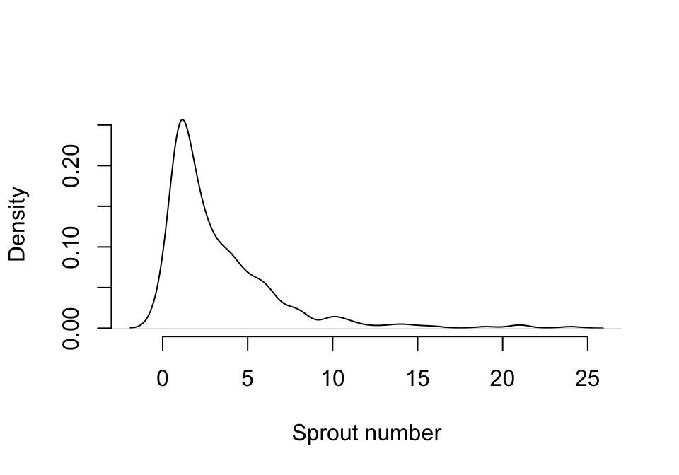
Figure 5.2: Density distribution of size in Cypripedium candidum
If size or fecundity is a count variable, then it should be set to the Poisson distribution if the mean does not differ significantly from the variance, and this can be tested with the hfv_qc() function. The negative binomial distribution is provided in cases where the assumption that the mean equals the variance is clearly broken. We do not encourage the use of the negative binomial except in such cases, as the extra parameters estimated for the negative binomial distribution reduce the power of the modeling exercises conducted.
The Poisson and the negative binomial distributions both predict specific numbers of zeros in the response variable. If excess zeros occur within the dataset even after including the observation status and reproductive status as vital rates to absorb zeros, then a zero-inflated Poisson or negative binomial distribution may be used. These modeling approaches work by parameterizing two separate models. The first is a binomial model, typically assuming a logit link, to predict excess zero responses. The second model is called a conditional model, and it is the Poisson or negative binomial model that is used to predict non-zero and only some zero responses. In effect, a zero-inflated model is actually two models in which zeros are assumed to result from two different processes, only one of which can result in non-zero counts. Because an extra model is built to cover excess zeros, zero-inflated models are much more complex and can include many more parameters than their non-inflated counterparts. The principle of parsimony suggests that they should only be used when there are significantly more zeros than expected.
Cases may arise in which zeros do not occur in either size or fecundity. For these situations, we provide zero-truncated distributions. This may occur in size if all cases of size = 0 are absorbed by observation status, leaving only positive integers for the size of observed individuals. For example, if an unobservable stage such as vegetative dormancy occurs and absorbs all cases of size = 0, then a zero-truncated Poisson or negative binomial distribution will be more appropriate than the equivalent distribution without zero-truncation. It can also occur if all cases of fecundity = 0 are absorbed by reproductive status. Such distributions only involve the estimation of single, conditional models, and so are simpler than zero-inflated models.
We have assumed that users will only use a single size variable in classification. However, cases may arise in which stages are classified under two or three size variables, and these two or three size variables are also used in vital rate modeling. These size variables can be treated as independent for the purposes of modeling, meaning that they can also have completely different distributions.
Let’s now build some function-based MPMs.
5.5 Using lefkoMod objects to create function-based MPMs
MPM creation from a demographic dataset can be accomplished with nine different functions:
rlefko2()- Creates raw ahistorical MPMs given a dataset, a stageframe, and a supplement table.rlefko3()- Creates raw historical MPMs given a dataset, a stageframe, and a supplement table.arlefko2()- Creates raw ahistorical age x stage MPMs given a dataset, a stageframe, and a supplement table.rleslie()- Creates raw age-based (Leslie) MPMs given a dataset.flefko2()- Creates function-based ahistorical MPMs given a dataset, a set of models, a stageframe, and a supplement table.flefko3()- Creates function-based historical MPMs given a dataset, a set of models, a stageframe, and a supplement table.aflefko2()- Creates function-based ahistorical age x stage MPMs given a dataset, a set of models, a stageframe, and a supplement table.fleslie()- Creates function-based age-based (Leslie) MPMs given a dataset and a set of models.mpm_create()- A general, all-purpose MPM creation function. All other MPM creation functions are actually wrappers for this function.
These functions incorporate binary kernels developed to handle the estimation of matrix elements quickly and efficiently. A single run of flefko3(), for example, should be able to yield all annual historical matrices for all patches for the Cypripedium candidum dataset provided with lefko3 in under a minute on most machines (14s or so on the author’s 2019 MacBook Pro with 2.3 GHz 8-Core Intel Core i9), while a single run of flefko2() should typically run in a fraction of a second. Parallel computing should not be necessary even with the slowest of current machines, provided that the machine is current enough to handle at least R 4.3.0.
The output for each of these functions is a lefkoMat object, which is an S3 object and is described in detail in Chapter 4. These lists include elements \(\mathbf{A}\), \(\mathbf{U}\), and \(\mathbf{F}\), which are themselves lists of complete projection matrices, survival-transition matrices, and fecundity matrices, respectively. For example, code such as matobject$A[[1]] would access the first complete projection matrix in a lefkoMat object named matobject. They are followed by elements referred to as ahstages, hstages, and agestages, which provide data frames describing the stages (technically showing the edited stageframe), the historical stage-pairs, and the age-stage pairs shown in the order in which they occur within the matrices, respectively. The labels element is a data frame giving a description of each matrix in the order in which it occurs within the \(\mathbf{A}\), \(\mathbf{U}\), and \(\mathbf{F}\) elements, including the population, patch, and monitoring time (time t) designations. The final elements are quality control outputs that vary in content depending on whether the output matrices are raw or function-based, but nonetheless always include at least the numbers of individuals and individual-transitions used for estimation.
Let’s create function-based MPMs with the lefkoMod objects that we created in this chapter. We will start with the ahistorical function-based MPM. We will also look at a summary of the resulting lefkoMat object, described in section 1.7.1.
cypmatrix2fp <- flefko2(stageframe = cypframe_fb, supplement = cypsupp2_fb,
  modelsuite = cypmodels2p, data = cypfb_v1)

summary(cypmatrix2fp)
>
> This ahistorical lefkoMat object contains 15 matrices.
>
> Each matrix is square with 54 rows and columns, and a total of 2916 elements.
> A total of 36165 survival transitions were estimated, with 2411 per matrix.
> A total of 720 fecundity transitions were estimated, with 48 per matrix.
> This lefkoMat object covers 1 population, 3 patches, and 5 time steps.
>
> The dataset contains a total of 74 unique individuals and 320 unique transitions.
>
> Vital rate modeling quality control:
>
> Survival estimated with 74 individuals and 320 individual transitions.
> Observation estimated with 70 individuals and 303 individual transitions.
> Primary size estimated with 70 individuals and 288 individual transitions.
> Secondary size transition not estimated.
> Tertiary size transition not estimated.
> Reproductive status estimated with 70 individuals and 288 individual transitions.
> Fecundity estimated with 51 individuals and 118 individual transitions.
> Juvenile survival not estimated.
> Juvenile observation probability not estimated.
> Juvenile primary size transition not estimated.
> Juvenile secondary size transition not estimated.
> Juvenile tertiary size transition not estimated.
> Juvenile reproduction probability not estimated.
> Juvenile maturity transition probability not estimated.
>
> Survival probability sum check (each matrix represented by column in order):
>          [,1]  [,2]  [,3]  [,4]  [,5]  [,6]  [,7]  [,8]  [,9] [,10] [,11] [,12]
> Min.    0.050 0.050 0.050 0.050 0.050 0.050 0.050 0.050 0.050 0.050 0.050 0.050
> 1st Qu. 0.991 0.991 0.991 0.991 0.991 0.991 0.991 0.991 0.991 0.991 0.991 0.991
> Median  1.000 1.000 1.000 1.000 1.000 1.000 1.000 1.000 1.000 1.000 1.000 1.000
> Mean    0.916 0.917 0.917 0.917 0.914 0.916 0.917 0.917 0.917 0.914 0.914 0.916
> 3rd Qu. 1.000 1.000 1.000 1.000 1.000 1.000 1.000 1.000 1.000 1.000 1.000 1.000
> Max.    1.000 1.000 1.000 1.000 1.000 1.000 1.000 1.000 1.000 1.000 1.000 1.000
>         [,13] [,14] [,15]
> Min.    0.050 0.050 0.050
> 1st Qu. 0.991 0.991 0.991
> Median  1.000 1.000 1.000
> Mean    0.916 0.916 0.913
> 3rd Qu. 1.000 1.000 1.000
> Max.    1.000 1.000 1.000
>
>
> All matrices have no stage discontinuities.
Here we have fifteen matrices. Since there are six years of data, there are a total of five pairs of consecutive years with which to estimate transitions. There are also three patches, yielding fifteen total matrices. We also have \(54^{2} = 2916\) elements per matrix, of which 2459 elements are estimated (the rest are zeros). Let’s look at the first function-based matrix.
print(cypmatrix2fp$A[[1]], digits = 3)
>       [,1] [,2] [,3] [,4]   [,5]     [,6]     [,7]     [,8]     [,9]    [,10]
>  [1,] 0.08  0.0  0.0 0.00 0.0000 0.00e+00 0.00e+00 0.00e+00 0.00e+00 0.00e+00
>  [2,] 0.10  0.0  0.0 0.00 0.0000 0.00e+00 0.00e+00 0.00e+00 0.00e+00 0.00e+00
>  [3,] 0.00  0.1  0.0 0.00 0.0000 0.00e+00 0.00e+00 0.00e+00 0.00e+00 0.00e+00
>  [4,] 0.00  0.0  0.1 0.00 0.0000 0.00e+00 0.00e+00 0.00e+00 0.00e+00 0.00e+00
>  [5,] 0.00  0.0  0.0 0.05 0.0500 0.00e+00 0.00e+00 0.00e+00 0.00e+00 0.00e+00
>  [6,] 0.00  0.0  0.0 0.00 0.0329 4.70e-02 3.69e-02 2.81e-02 2.10e-02 1.56e-02
>  [7,] 0.00  0.0  0.0 0.00 0.1628 2.33e-01 2.38e-01 2.36e-01 2.28e-01 2.17e-01
>  [8,] 0.00  0.0  0.0 0.00 0.1035 1.48e-01 1.52e-01 1.50e-01 1.45e-01 1.38e-01
>  [9,] 0.00  0.0  0.0 0.00 0.0658 9.40e-02 9.64e-02 9.54e-02 9.23e-02 8.77e-02
> [10,] 0.00  0.0  0.0 0.00 0.0000 5.98e-02 6.13e-02 6.07e-02 5.87e-02 5.58e-02
> [11,] 0.00  0.0  0.0 0.00 0.0000 3.80e-02 3.90e-02 3.86e-02 3.73e-02 3.55e-02
> [12,] 0.00  0.0  0.0 0.00 0.0000 2.42e-02 2.48e-02 2.45e-02 2.37e-02 2.25e-02
> [13,] 0.00  0.0  0.0 0.00 0.0000 1.54e-02 1.58e-02 1.56e-02 1.51e-02 1.43e-02
> [14,] 0.00  0.0  0.0 0.00 0.0000 9.78e-03 1.00e-02 9.92e-03 9.59e-03 9.12e-03
> [15,] 0.00  0.0  0.0 0.00 0.0000 6.22e-03 6.38e-03 6.31e-03 6.10e-03 5.80e-03
> [16,] 0.00  0.0  0.0 0.00 0.0000 3.96e-03 4.05e-03 4.01e-03 3.88e-03 3.69e-03
> [17,] 0.00  0.0  0.0 0.00 0.0000 2.52e-03 2.58e-03 2.55e-03 2.47e-03 2.34e-03
> [18,] 0.00  0.0  0.0 0.00 0.0000 1.60e-03 1.64e-03 1.62e-03 1.57e-03 1.49e-03
>          [,11]    [,12]    [,13]    [,14]    [,15]    [,16]    [,17]    [,18]
>  [1,] 0.00e+00 0.00e+00 0.00e+00 0.00e+00 0.00e+00 0.00e+00 0.00e+00 0.00e+00
>  [2,] 0.00e+00 0.00e+00 0.00e+00 0.00e+00 0.00e+00 0.00e+00 0.00e+00 0.00e+00
>  [3,] 0.00e+00 0.00e+00 0.00e+00 0.00e+00 0.00e+00 0.00e+00 0.00e+00 0.00e+00
>  [4,] 0.00e+00 0.00e+00 0.00e+00 0.00e+00 0.00e+00 0.00e+00 0.00e+00 0.00e+00
>  [5,] 0.00e+00 0.00e+00 0.00e+00 0.00e+00 0.00e+00 0.00e+00 0.00e+00 0.00e+00
>  [6,] 1.15e-02 8.47e-03 6.21e-03 4.55e-03 3.33e-03 2.44e-03 1.78e-03 1.30e-03
>  [7,] 2.03e-01 1.89e-01 1.73e-01 1.57e-01 1.42e-01 1.27e-01 1.13e-01 9.94e-02
>  [8,] 1.29e-01 1.20e-01 1.10e-01 1.00e-01 9.03e-02 8.08e-02 7.17e-02 6.32e-02
>  [9,] 8.22e-02 7.62e-02 7.00e-02 6.37e-02 5.74e-02 5.14e-02 4.56e-02 4.02e-02
> [10,] 5.23e-02 4.85e-02 4.45e-02 4.05e-02 3.65e-02 3.27e-02 2.90e-02 2.56e-02
> [11,] 3.32e-02 3.08e-02 2.83e-02 2.57e-02 2.32e-02 2.08e-02 1.84e-02 1.63e-02
> [12,] 2.11e-02 1.96e-02 1.80e-02 1.64e-02 1.48e-02 1.32e-02 1.17e-02 1.03e-02
> [13,] 1.34e-02 1.25e-02 1.14e-02 1.04e-02 9.39e-03 8.40e-03 7.46e-03 6.57e-03
> [14,] 8.55e-03 7.93e-03 7.28e-03 6.62e-03 5.97e-03 5.34e-03 4.74e-03 4.18e-03
> [15,] 5.44e-03 5.04e-03 4.63e-03 4.21e-03 3.80e-03 3.40e-03 3.02e-03 2.66e-03
> [16,] 3.46e-03 3.21e-03 2.94e-03 2.68e-03 2.41e-03 2.16e-03 1.92e-03 1.69e-03
> [17,] 2.20e-03 2.04e-03 1.87e-03 1.70e-03 1.54e-03 1.37e-03 1.22e-03 1.08e-03
> [18,] 1.40e-03 1.30e-03 1.19e-03 1.08e-03 9.77e-04 8.74e-04 7.76e-04 6.84e-04
>          [,19]    [,20]    [,21]    [,22]    [,23]    [,24]    [,25]    [,26]
>  [1,] 0.00e+00 0.00e+00 0.00e+00 0.00e+00 0.00e+00 0.00e+00 0.00e+00 0.00e+00
>  [2,] 0.00e+00 0.00e+00 0.00e+00 0.00e+00 0.00e+00 0.00e+00 0.00e+00 0.00e+00
>  [3,] 0.00e+00 0.00e+00 0.00e+00 0.00e+00 0.00e+00 0.00e+00 0.00e+00 0.00e+00
>  [4,] 0.00e+00 0.00e+00 0.00e+00 0.00e+00 0.00e+00 0.00e+00 0.00e+00 0.00e+00
>  [5,] 0.00e+00 0.00e+00 0.00e+00 0.00e+00 0.00e+00 0.00e+00 0.00e+00 0.00e+00
>  [6,] 9.54e-04 6.97e-04 5.10e-04 3.73e-04 2.72e-04 1.99e-04 1.46e-04 1.06e-04
>  [7,] 8.70e-02 7.58e-02 6.56e-02 5.66e-02 4.85e-02 4.15e-02 3.54e-02 3.01e-02
>  [8,] 5.54e-02 4.82e-02 4.17e-02 3.60e-02 3.09e-02 2.64e-02 2.25e-02 1.91e-02
>  [9,] 3.52e-02 3.06e-02 2.65e-02 2.29e-02 1.96e-02 1.68e-02 1.43e-02 1.22e-02
> [10,] 2.24e-02 1.95e-02 1.69e-02 1.45e-02 1.25e-02 1.07e-02 9.10e-03 7.73e-03
> [11,] 1.42e-02 1.24e-02 1.07e-02 9.25e-03 7.94e-03 6.79e-03 5.79e-03 4.92e-03
> [12,] 9.05e-03 7.88e-03 6.83e-03 5.88e-03 5.05e-03 4.32e-03 3.68e-03 3.13e-03
> [13,] 5.76e-03 5.01e-03 4.34e-03 3.74e-03 3.21e-03 2.75e-03 2.34e-03 1.99e-03
> [14,] 3.66e-03 3.19e-03 2.76e-03 2.38e-03 2.04e-03 1.75e-03 1.49e-03 1.26e-03
> [15,] 2.33e-03 2.03e-03 1.76e-03 1.51e-03 1.30e-03 1.11e-03 9.46e-04 8.04e-04
> [16,] 1.48e-03 1.29e-03 1.12e-03 9.62e-04 8.26e-04 7.06e-04 6.02e-04 5.11e-04
> [17,] 9.42e-04 8.20e-04 7.10e-04 6.12e-04 5.25e-04 4.49e-04 3.83e-04 3.25e-04
> [18,] 5.99e-04 5.21e-04 4.51e-04 3.89e-04 3.34e-04 2.86e-04 2.43e-04 2.07e-04
>          [,27]    [,28]    [,29]    [,30]    [,31]    [,32]    [,33]    [,34]
>  [1,] 0.00e+00 0.00e+00 0.00e+00 0.00e+00 8.13e+02 8.13e+02 8.13e+02 8.13e+02
>  [2,] 0.00e+00 0.00e+00 0.00e+00 0.00e+00 8.13e+02 8.13e+02 8.13e+02 8.13e+02
>  [3,] 0.00e+00 0.00e+00 0.00e+00 0.00e+00 0.00e+00 0.00e+00 0.00e+00 0.00e+00
>  [4,] 0.00e+00 0.00e+00 0.00e+00 0.00e+00 0.00e+00 0.00e+00 0.00e+00 0.00e+00
>  [5,] 0.00e+00 0.00e+00 0.00e+00 0.00e+00 0.00e+00 0.00e+00 0.00e+00 0.00e+00
>  [6,] 7.78e-05 5.69e-05 4.16e-05 3.04e-05 3.69e-02 2.81e-02 2.10e-02 1.56e-02
>  [7,] 2.55e-02 2.16e-02 1.82e-02 1.54e-02 1.18e-01 1.10e-01 9.94e-02 8.85e-02
>  [8,] 1.62e-02 1.37e-02 1.16e-02 9.77e-03 7.54e-02 6.98e-02 6.32e-02 5.63e-02
>  [9,] 1.03e-02 8.72e-03 7.36e-03 6.21e-03 4.79e-02 4.44e-02 4.02e-02 3.58e-02
> [10,] 6.56e-03 5.55e-03 4.68e-03 3.95e-03 3.05e-02 2.82e-02 2.56e-02 2.27e-02
> [11,] 4.17e-03 3.53e-03 2.98e-03 2.51e-03 1.94e-02 1.80e-02 1.63e-02 1.45e-02
> [12,] 2.65e-03 2.24e-03 1.89e-03 1.60e-03 1.23e-02 1.14e-02 1.03e-02 9.20e-03
> [13,] 1.69e-03 1.43e-03 1.20e-03 1.02e-03 7.84e-03 7.26e-03 6.57e-03 5.85e-03
> [14,] 1.07e-03 9.07e-04 7.66e-04 6.46e-04 4.98e-03 4.62e-03 4.18e-03 3.72e-03
> [15,] 6.82e-04 5.77e-04 4.87e-04 4.11e-04 3.17e-03 2.94e-03 2.66e-03 2.37e-03
> [16,] 4.34e-04 3.67e-04 3.10e-04 2.61e-04 2.02e-03 1.87e-03 1.69e-03 1.50e-03
> [17,] 2.76e-04 2.33e-04 1.97e-04 1.66e-04 1.28e-03 1.19e-03 1.07e-03 9.57e-04
> [18,] 1.75e-04 1.48e-04 1.25e-04 1.06e-04 8.15e-04 7.55e-04 6.83e-04 6.08e-04
>          [,35]    [,36]    [,37]    [,38]    [,39]    [,40]    [,41]    [,42]
>  [1,] 8.13e+02 8.13e+02 8.13e+02 8.13e+02 8.13e+02 8.13e+02 8.13e+02 8.13e+02
>  [2,] 8.13e+02 8.13e+02 8.13e+02 8.13e+02 8.13e+02 8.13e+02 8.13e+02 8.13e+02
>  [3,] 0.00e+00 0.00e+00 0.00e+00 0.00e+00 0.00e+00 0.00e+00 0.00e+00 0.00e+00
>  [4,] 0.00e+00 0.00e+00 0.00e+00 0.00e+00 0.00e+00 0.00e+00 0.00e+00 0.00e+00
>  [5,] 0.00e+00 0.00e+00 0.00e+00 0.00e+00 0.00e+00 0.00e+00 0.00e+00 0.00e+00
>  [6,] 1.15e-02 8.47e-03 6.21e-03 4.55e-03 3.33e-03 2.44e-03 1.78e-03 1.30e-03
>  [7,] 7.78e-02 6.79e-02 5.88e-02 5.06e-02 4.34e-02 3.71e-02 3.15e-02 2.68e-02
>  [8,] 4.95e-02 4.32e-02 3.74e-02 3.22e-02 2.76e-02 2.36e-02 2.01e-02 1.70e-02
>  [9,] 3.15e-02 2.74e-02 2.38e-02 2.05e-02 1.76e-02 1.50e-02 1.28e-02 1.08e-02
> [10,] 2.00e-02 1.75e-02 1.51e-02 1.30e-02 1.12e-02 9.53e-03 8.11e-03 6.89e-03
> [11,] 1.27e-02 1.11e-02 9.61e-03 8.28e-03 7.10e-03 6.06e-03 5.16e-03 4.38e-03
> [12,] 8.09e-03 7.06e-03 6.11e-03 5.27e-03 4.51e-03 3.85e-03 3.28e-03 2.79e-03
> [13,] 5.15e-03 4.49e-03 3.89e-03 3.35e-03 2.87e-03 2.45e-03 2.09e-03 1.77e-03
> [14,] 3.27e-03 2.85e-03 2.47e-03 2.13e-03 1.83e-03 1.56e-03 1.33e-03 1.13e-03
> [15,] 2.08e-03 1.82e-03 1.57e-03 1.35e-03 1.16e-03 9.91e-04 8.44e-04 7.16e-04
> [16,] 1.32e-03 1.15e-03 1.00e-03 8.61e-04 7.38e-04 6.30e-04 5.37e-04 4.55e-04
> [17,] 8.42e-04 7.34e-04 6.36e-04 5.48e-04 4.69e-04 4.01e-04 3.41e-04 2.90e-04
> [18,] 5.35e-04 4.67e-04 4.04e-04 3.48e-04 2.99e-04 2.55e-04 2.17e-04 1.84e-04
>          [,43]    [,44]    [,45]    [,46]    [,47]    [,48]    [,49]    [,50]
>  [1,] 8.13e+02 8.13e+02 8.13e+02 8.13e+02 8.13e+02 8.13e+02 8.13e+02 8.13e+02
>  [2,] 8.13e+02 8.13e+02 8.13e+02 8.13e+02 8.13e+02 8.13e+02 8.13e+02 8.13e+02
>  [3,] 0.00e+00 0.00e+00 0.00e+00 0.00e+00 0.00e+00 0.00e+00 0.00e+00 0.00e+00
>  [4,] 0.00e+00 0.00e+00 0.00e+00 0.00e+00 0.00e+00 0.00e+00 0.00e+00 0.00e+00
>  [5,] 0.00e+00 0.00e+00 0.00e+00 0.00e+00 0.00e+00 0.00e+00 0.00e+00 0.00e+00
>  [6,] 9.54e-04 6.97e-04 5.10e-04 3.73e-04 2.72e-04 1.99e-04 1.46e-04 1.06e-04
>  [7,] 2.27e-02 1.92e-02 1.62e-02 1.36e-02 1.15e-02 9.64e-03 8.10e-03 6.80e-03
>  [8,] 1.44e-02 1.22e-02 1.03e-02 8.66e-03 7.29e-03 6.13e-03 5.15e-03 4.32e-03
>  [9,] 9.17e-03 7.75e-03 6.54e-03 5.51e-03 4.64e-03 3.90e-03 3.27e-03 2.75e-03
> [10,] 5.83e-03 4.93e-03 4.16e-03 3.50e-03 2.95e-03 2.48e-03 2.08e-03 1.75e-03
> [11,] 3.71e-03 3.13e-03 2.64e-03 2.23e-03 1.88e-03 1.58e-03 1.32e-03 1.11e-03
> [12,] 2.36e-03 1.99e-03 1.68e-03 1.42e-03 1.19e-03 1.00e-03 8.42e-04 7.07e-04
> [13,] 1.50e-03 1.27e-03 1.07e-03 9.01e-04 7.58e-04 6.38e-04 5.36e-04 4.50e-04
> [14,] 9.54e-04 8.06e-04 6.80e-04 5.73e-04 4.82e-04 4.05e-04 3.41e-04 2.86e-04
> [15,] 6.07e-04 5.13e-04 4.33e-04 3.64e-04 3.07e-04 2.58e-04 2.17e-04 1.82e-04
> [16,] 3.86e-04 3.26e-04 2.75e-04 2.32e-04 1.95e-04 1.64e-04 1.38e-04 1.16e-04
> [17,] 2.45e-04 2.07e-04 1.75e-04 1.47e-04 1.24e-04 1.04e-04 8.76e-05 7.35e-05
> [18,] 1.56e-04 1.32e-04 1.11e-04 9.37e-05 7.89e-05 6.63e-05 5.57e-05 4.68e-05
>          [,51]    [,52]    [,53]    [,54]
>  [1,] 8.13e+02 8.13e+02 8.13e+02 8.13e+02
>  [2,] 8.13e+02 8.13e+02 8.13e+02 8.13e+02
>  [3,] 0.00e+00 0.00e+00 0.00e+00 0.00e+00
>  [4,] 0.00e+00 0.00e+00 0.00e+00 0.00e+00
>  [5,] 0.00e+00 0.00e+00 0.00e+00 0.00e+00
>  [6,] 7.78e-05 5.69e-05 4.16e-05 3.04e-05
>  [7,] 5.70e-03 4.78e-03 4.01e-03 3.36e-03
>  [8,] 3.63e-03 3.04e-03 2.55e-03 2.13e-03
>  [9,] 2.31e-03 1.93e-03 1.62e-03 1.36e-03
> [10,] 1.47e-03 1.23e-03 1.03e-03 8.63e-04
> [11,] 9.32e-04 7.82e-04 6.55e-04 5.49e-04
> [12,] 5.93e-04 4.97e-04 4.17e-04 3.49e-04
> [13,] 3.77e-04 3.16e-04 2.65e-04 2.22e-04
> [14,] 2.40e-04 2.01e-04 1.69e-04 1.41e-04
> [15,] 1.53e-04 1.28e-04 1.07e-04 8.98e-05
> [16,] 9.70e-05 8.13e-05 6.82e-05 5.71e-05
> [17,] 6.17e-05 5.17e-05 4.33e-05 3.63e-05
> [18,] 3.92e-05 3.29e-05 2.76e-05 2.31e-05
>  [ reached 'max' / getOption("max.print") -- omitted 36 rows ]
Notice that this matrix is bigger and more full of non-zero values than the associated raw matrix. This is due to the fact that function-based matrices use kernels to estimate every estimable element, while raw matrices are populated only by proportions of individuals making actual transitions. Thus, if no individuals make a particular transition, then a raw matrix will assign that survival-transition probability a zero, while a function-based matrix will provide a non-zero estimate based on the chosen vital rate linear models.
Let’s now estimate the function-based historical MPM. Because this will have huge dimensions, we will set sparse_output = TRUE to make sure that it does not take up too much memory (standard matrix format should yield a lefkoMat object taking up over three gigabytes, while the sparse matrix format should yield a lefkoMat object taking up only a little over 40 megabytes).
cypmatrix3fp <- flefko3(stageframe = cypframe_fb, supplement = cypsupp3_fb,
  modelsuite = cypmodels3p, data = cypfb_v1, sparse_output = TRUE)

summary(cypmatrix3fp)
>
> This historical lefkoMat object contains 15 matrices.
>
> Each matrix is square with 2916 rows and columns, and a total of 8503056 elements.
> A total of 1768620 survival transitions were estimated, with 117908 per matrix.
> A total of 35280 fecundity transitions were estimated, with 2352 per matrix.
> This lefkoMat object covers 1 population, 3 patches, and 5 time steps.
>
> The dataset contains a total of 74 unique individuals and 320 unique transitions.
>
> Vital rate modeling quality control:
>
> Survival estimated with 74 individuals and 320 individual transitions.
> Observation estimated with 70 individuals and 303 individual transitions.
> Primary size estimated with 70 individuals and 288 individual transitions.
> Secondary size transition not estimated.
> Tertiary size transition not estimated.
> Reproductive status estimated with 70 individuals and 288 individual transitions.
> Fecundity estimated with 51 individuals and 118 individual transitions.
> Juvenile survival not estimated.
> Juvenile observation probability not estimated.
> Juvenile primary size transition not estimated.
> Juvenile secondary size transition not estimated.
> Juvenile tertiary size transition not estimated.
> Juvenile reproduction probability not estimated.
> Juvenile maturity transition probability not estimated.
>
> Survival probability sum check (each matrix represented by column in order):
>          [,1]  [,2]  [,3]  [,4]  [,5]  [,6]  [,7]  [,8]  [,9] [,10] [,11] [,12]
> Min.    0.000 0.000 0.000 0.000 0.000 0.000 0.000 0.000 0.000 0.000 0.000 0.000
> 1st Qu. 0.965 0.965 0.965 0.965 0.965 0.964 0.965 0.965 0.965 0.964 0.964 0.965
> Median  1.000 1.000 1.000 1.000 1.000 1.000 1.000 1.000 1.000 1.000 1.000 1.000
> Mean    0.820 0.820 0.820 0.820 0.820 0.820 0.820 0.820 0.820 0.820 0.820 0.820
> 3rd Qu. 1.000 1.000 1.000 1.000 1.000 1.000 1.000 1.000 1.000 1.000 1.000 1.000
> Max.    1.000 1.000 1.000 1.000 1.000 1.000 1.000 1.000 1.000 1.000 1.000 1.000
>         [,13] [,14] [,15]
> Min.    0.000 0.000 0.000
> 1st Qu. 0.965 0.964 0.964
> Median  1.000 1.000 1.000
> Mean    0.820 0.820 0.820
> 3rd Qu. 1.000 1.000 1.000
> Max.    1.000 1.000 1.000
>
>
> Stage-pairs without connections leading to them found in matrices: 1 2 3 4 5 6 7 8 9 10 11 12 13 14 15
Notice the similarities and differences with the ahistorical MPMs. First, we see 15 matrices produced again. Second, these matrices are utterly huge. They have \(54^2 = 2916\) rows and columns, yielding \(2916^2 = 8,503,056\) total elements per matrix. And we have 120,260 elements estimated per matrix. This is vastly more than in the ahistorical case. However, it is also just a small fraction of the total number of elements in the matrix. In fact, in an unreduced hMPM estimated in Ehrlén format, the total number of elements that can be estimated is equal to \(\frac{r \times c}{m}\), where \(r\) and \(c\) are the numbers of rows and columns, respectively, and \(m\) is the number of stages in the stageframe. For example, if there are 10 stages in the stageframe, then only 1000 of the total 10,000 elements in the hMPM are estimable (10% of the elements).
We can also make deVries format hMPMs. Here, we just add a single option regarding format. The resulting summary shows bigger matrices, reflecting the addition of the prior stage for newborns.
cypmatrix3fp_deV <- flefko3(stageframe = cypframe_fb, supplement = cypsupp3_fb,
  modelsuite = cypmodels3p, data = cypfb_v1, format = "deVries",
  sparse_output = TRUE)

summary(cypmatrix3fp_deV)
>
> This historical lefkoMat object contains 15 matrices.
>
> Each matrix is square with 2970 rows and columns, and a total of 8820900 elements.
> A total of 1767900 survival transitions were estimated, with 117860 per matrix.
> A total of 35280 fecundity transitions were estimated, with 2352 per matrix.
> This lefkoMat object covers 1 population, 3 patches, and 5 time steps.
>
> The dataset contains a total of 74 unique individuals and 320 unique transitions.
>
> Vital rate modeling quality control:
>
> Survival estimated with 74 individuals and 320 individual transitions.
> Observation estimated with 70 individuals and 303 individual transitions.
> Primary size estimated with 70 individuals and 288 individual transitions.
> Secondary size transition not estimated.
> Tertiary size transition not estimated.
> Reproductive status estimated with 70 individuals and 288 individual transitions.
> Fecundity estimated with 51 individuals and 118 individual transitions.
> Juvenile survival not estimated.
> Juvenile observation probability not estimated.
> Juvenile primary size transition not estimated.
> Juvenile secondary size transition not estimated.
> Juvenile tertiary size transition not estimated.
> Juvenile reproduction probability not estimated.
> Juvenile maturity transition probability not estimated.
>
> Survival probability sum check (each matrix represented by column in order):
>          [,1]  [,2]  [,3]  [,4]  [,5]  [,6]  [,7]  [,8]  [,9] [,10] [,11] [,12]
> Min.    0.000 0.000 0.000 0.000 0.000 0.000 0.000 0.000 0.000 0.000 0.000 0.000
> 1st Qu. 0.965 0.965 0.965 0.965 0.965 0.964 0.965 0.965 0.965 0.964 0.964 0.965
> Median  1.000 1.000 1.000 1.000 1.000 0.999 1.000 1.000 1.000 0.999 0.999 1.000
> Mean    0.804 0.804 0.804 0.804 0.803 0.803 0.804 0.804 0.804 0.803 0.803 0.804
> 3rd Qu. 1.000 1.000 1.000 1.000 1.000 1.000 1.000 1.000 1.000 1.000 1.000 1.000
> Max.    1.000 1.000 1.000 1.000 1.000 1.000 1.000 1.000 1.000 1.000 1.000 1.000
>         [,13] [,14] [,15]
> Min.    0.000 0.000 0.000
> 1st Qu. 0.965 0.964 0.964
> Median  0.999 0.999 0.999
> Mean    0.804 0.803 0.803
> 3rd Qu. 1.000 1.000 1.000
> Max.    1.000 1.000 1.000
>
>
> Stage-pairs without connections leading to them found in matrices: 1 2 3 4 5 6 7 8 9 10 11 12 13 14 15
Now that we have created our MPMs, we might wish to create element-wise arithmetic mean matrices to aid inference and further analysis. For example, we might be interested in developing patch-level means and an overall population mean, but one in which the element means treat each patch and each year as equal in proportional effect. For this purpose, we can use the lmean() function.
cyp2fp_mean <- lmean(cypmatrix2fp)
cyp3fp_mean <- lmean(cypmatrix3fp)

summary(cyp2fp_mean)
>
> This ahistorical lefkoMat object contains 4 matrices.
>
> Each matrix is square with 54 rows and columns, and a total of 2916 elements.
> A total of 9644 survival transitions were estimated, with 2411 per matrix.
> A total of 192 fecundity transitions were estimated, with 48 per matrix.
> This lefkoMat object covers 1 population, 4 patches, and 0 time steps.
>
> The dataset contains a total of 74 unique individuals and 320 unique transitions.
>
> Vital rate modeling quality control:
>
> Survival estimated with 74 individuals and 320 individual transitions.
> Observation estimated with 70 individuals and 303 individual transitions.
> Primary size estimated with 70 individuals and 288 individual transitions.
> Secondary size transition not estimated.
> Tertiary size transition not estimated.
> Reproductive status estimated with 70 individuals and 288 individual transitions.
> Fecundity estimated with 51 individuals and 118 individual transitions.
> Juvenile survival not estimated.
> Juvenile observation probability not estimated.
> Juvenile primary size transition not estimated.
> Juvenile secondary size transition not estimated.
> Juvenile tertiary size transition not estimated.
> Juvenile reproduction probability not estimated.
> Juvenile maturity transition probability not estimated.
>
> Survival probability sum check (each matrix represented by column in order):
>          [,1]  [,2]  [,3]  [,4]
> Min.    0.050 0.050 0.050 0.050
> 1st Qu. 0.991 0.991 0.991 0.991
> Median  1.000 1.000 1.000 1.000
> Mean    0.916 0.916 0.915 0.916
> 3rd Qu. 1.000 1.000 1.000 1.000
> Max.    1.000 1.000 1.000 1.000
>
>
> All matrices have no stage discontinuities.
summary(cyp3fp_mean)
>
> This historical lefkoMat object contains 4 matrices.
>
> Each matrix is square with 2916 rows and columns, and a total of 8503056 elements.
> A total of 471632 survival transitions were estimated, with 117908 per matrix.
> A total of 9408 fecundity transitions were estimated, with 2352 per matrix.
> This lefkoMat object covers 1 population, 4 patches, and 0 time steps.
>
> The dataset contains a total of 74 unique individuals and 320 unique transitions.
>
> Vital rate modeling quality control:
>
> Survival estimated with 74 individuals and 320 individual transitions.
> Observation estimated with 70 individuals and 303 individual transitions.
> Primary size estimated with 70 individuals and 288 individual transitions.
> Secondary size transition not estimated.
> Tertiary size transition not estimated.
> Reproductive status estimated with 70 individuals and 288 individual transitions.
> Fecundity estimated with 51 individuals and 118 individual transitions.
> Juvenile survival not estimated.
> Juvenile observation probability not estimated.
> Juvenile primary size transition not estimated.
> Juvenile secondary size transition not estimated.
> Juvenile tertiary size transition not estimated.
> Juvenile reproduction probability not estimated.
> Juvenile maturity transition probability not estimated.
>
> Survival probability sum check (each matrix represented by column in order):
>          [,1]  [,2]  [,3]  [,4]
> Min.    0.000 0.000 0.000 0.000
> 1st Qu. 0.965 0.965 0.964 0.965
> Median  1.000 1.000 1.000 1.000
> Mean    0.820 0.820 0.820 0.820
> 3rd Qu. 1.000 1.000 1.000 1.000
> Max.    1.000 1.000 1.000 1.000
>
>
> Stage-pairs without connections leading to them found in matrices: 1 2 3 4
The function-based mean matrices have the same number of estimated transitions as their constituent matrices, because all elements that are estimable are actually estimated using the vital rate models supplied, meaning that each matrix used per mean has the same number of estimated elements. We have four mean matrices in each case - the first three are patch-level means for each of three patches, and the final matrix in each case is the population mean matrix. The labels element in each lefkoMat object shows this order.
In the preceding vital rate model sets, we created best-fit models that necessarily included a patch term. This will result necessarily in the creation of matrices at the patch level. To create matrices for the population level only, we remove the patch option from the preceding function calls, as below.
cypmodels3 <- modelsearch(cypfb_v1, historical = TRUE, approach = "mixed",
  vitalrates = c("surv", "obs", "size", "repst", "fec"),
  sizedist = "negbin", size.trunc = TRUE, fecdist = "poisson", fec.zero = TRUE,
  suite = "main", size = c("size3added", "size2added", "size1added"),
  quiet = "partial")

cypmodels2 <- modelsearch(cypfb_v1, historical = FALSE, approach = "mixed",
  vitalrates = c("surv", "obs", "size", "repst", "fec"),
  sizedist = "negbin", size.trunc = TRUE, fecdist = "poisson", fec.zero = TRUE,
  suite = "main", size = c("size3added", "size2added"),
  quiet = "partial")
Let’s see the model suite summaries. First the historical set.
summary(cypmodels3)
> This LefkoMod object includes 5 linear models.
> Best-fit model criterion used: aicc&k
>
>
>
> Survival model:
> Generalized linear mixed model fit by maximum likelihood (Laplace
>   Approximation) [glmerMod]
>  Family: binomial  ( logit )
> Formula: alive3 ~ size2added + (1 | year2) + (1 | individ)
>    Data: surv.data
>       AIC       BIC    logLik -2*log(L)  df.resid
>  128.1324  143.2057  -60.0662  120.1324       316
> Random effects:
>  Groups  Name        Std.Dev.
>  individ (Intercept) 1.198379
>  year2   (Intercept) 0.008826
> Number of obs: 320, groups:  individ, 74; year2, 5
> Fixed Effects:
> (Intercept)   size2added
>      2.0352       0.6344
> optimizer (Nelder_Mead) convergence code: 0 (OK) ; 0 optimizer warnings; 1 lme4 warnings
>
>
>
> Observation model:
> Generalized linear mixed model fit by maximum likelihood (Laplace
>   Approximation) [glmerMod]
>  Family: binomial  ( logit )
> Formula: obsstatus3 ~ size2added + (1 | year2) + (1 | individ)
>    Data: obs.data
>       AIC       BIC    logLik -2*log(L)  df.resid
>  118.2567  133.1117  -55.1284  110.2567       299
> Random effects:
>  Groups  Name        Std.Dev.
>  individ (Intercept) 1.078e-05
>  year2   (Intercept) 8.776e-01
> Number of obs: 303, groups:  individ, 70; year2, 5
> Fixed Effects:
> (Intercept)   size2added
>      2.4904       0.3134
> optimizer (Nelder_Mead) convergence code: 0 (OK) ; 0 optimizer warnings; 1 lme4 warnings
>
>
>
> Size model:
> Formula:          size3added ~ (1 | year2) + (1 | individ)
> Data: size.data
>       AIC       BIC    logLik -2*log(L)  df.resid
> 1008.2764 1022.9282 -500.1382 1000.2764       284
> Random-effects (co)variances:
>
> Conditional model:
>  Groups  Name        Std.Dev.
>  year2   (Intercept) 0.1109
>  individ (Intercept) 1.0561
>
> Number of obs: 288 / Conditional model: year2, 5; individ, 70
>
> Dispersion parameter for truncated_nbinom2 family (): 1.99e+07
>
> Fixed Effects:
>
> Conditional model:
> (Intercept)
>      0.5761
>
>
>
> Secondary size model:
> [1] 1
>
>
>
> Tertiary size model:
> [1] 1
>
>
>
> Reproductive status model:
> Generalized linear mixed model fit by maximum likelihood (Laplace
>   Approximation) [glmerMod]
>  Family: binomial  ( logit )
> Formula: repstatus3 ~ repstatus2 + size2added + (1 | year2) + (1 | individ)
>    Data: repst.data
>       AIC       BIC    logLik -2*log(L)  df.resid
>  333.6176  351.9324 -161.8088  323.6176       283
> Random effects:
>  Groups  Name        Std.Dev.
>  individ (Intercept) 0.1829
>  year2   (Intercept) 0.6250
> Number of obs: 288, groups:  individ, 70; year2, 5
> Fixed Effects:
> (Intercept)   repstatus2   size2added
>     -1.4631       1.6457       0.1715
>
>
>
> Fecundity model:
> Formula:          feca2 ~ size2added + (1 | year2) + (1 | individ)
> Zero inflation:         ~size2added + (1 | year2) + (1 | individ)
> Data: fec.data
>       AIC       BIC    logLik -2*log(L)  df.resid
>  248.8609  271.0264 -116.4305  232.8609       110
> Random-effects (co)variances:
>
> Conditional model:
>  Groups  Name        Std.Dev.
>  year2   (Intercept) 0.5760
>  individ (Intercept) 0.1639
>
> Zero-inflation model:
>  Groups  Name        Std.Dev.
>  year2   (Intercept) 1.642e-06
>  individ (Intercept) 3.089e-04
>
> Number of obs: 118 / Conditional model: year2, 5; individ, 51 / Zero-inflation model: year2, 5; individ, 51
>
> Fixed Effects:
>
> Conditional model:
> (Intercept)   size2added
>    -0.54014      0.06174
>
> Zero-inflation model:
> (Intercept)   size2added
>       3.865       -1.574
>
>
> Juvenile survival model:
> [1] 1
>
>
>
> Juvenile observation model:
> [1] 1
>
>
>
> Juvenile size model:
> [1] 1
>
>
>
> Juvenile secondary size model:
> [1] 1
>
>
>
> Juvenile tertiary size model:
> [1] 1
>
>
>
> Juvenile reproduction model:
> [1] 1
>
>
>
> Juvenile maturity model:
> [1] 1
>
>
>
>
>
> Number of models in survival table: 16
>
> Number of models in observation table: 16
>
> Number of models in size table: 16
>
> Number of models in secondary size table: 1
>
> Number of models in tertiary size table: 1
>
> Number of models in reproduction status table: 16
>
> Number of models in fecundity table: 256
>
> Number of models in juvenile survival table: 1
>
> Number of models in juvenile observation table: 1
>
> Number of models in juvenile size table: 1
>
> Number of models in juvenile secondary size table: 1
>
> Number of models in juvenile tertiary size table: 1
>
> Number of models in juvenile reproduction table: 1
>
> Number of models in juvenile maturity table: 1
>
>
>
>
>
> General model parameter names (column 1), and
> specific names used in these models (column 2):
>                       parameter_names mainparams
> 1                              time t      year2
> 2                          individual    individ
> 3                               patch      patch
> 4                   alive in time t+1      surv3
> 5                observed in time t+1       obs3
> 6                   sizea in time t+1      size3
> 7                   sizeb in time t+1     sizeb3
> 8                   sizec in time t+1     sizec3
> 9     reproductive status in time t+1     repst3
> 10              fecundity in time t+1       fec3
> 11                fecundity in time t       fec2
> 12                    sizea in time t      size2
> 13                  sizea in time t-1      size1
> 14                    sizeb in time t     sizeb2
> 15                  sizeb in time t-1     sizeb1
> 16                    sizec in time t     sizec2
> 17                  sizec in time t-1     sizec1
> 18      reproductive status in time t     repst2
> 19    reproductive status in time t-1     repst1
> 20        maturity status in time t+1     matst3
> 21          maturity status in time t     matst2
> 22                      age in time t        age
> 23                  density in time t    density
> 24   individual covariate a in time t   indcova2
> 25 individual covariate a in time t-1   indcova1
> 26   individual covariate b in time t   indcovb2
> 27 individual covariate b in time t-1   indcovb1
> 28   individual covariate c in time t   indcovc2
> 29 individual covariate c in time t-1   indcovc1
> 30              stage group in time t     group2
> 31            stage group in time t-1     group1
> 32       annual covariate a in time t  annucova2
> 33     annual covariate a in time t-1  annucova1
> 34       annual covariate b in time t  annucovb2
> 35     annual covariate b in time t-1  annucovb1
> 36       annual covariate c in time t  annucovc2
> 37     annual covariate c in time t-1  annucovc1
>
>
>
>
>
> Quality control:
>
> Survival model estimated with 74 individuals and 320 individual transitions.
> Survival model accuracy is 0.947.
> Observation status model estimated with 70 individuals and 303 individual transitions.
> Observation status model accuracy is 0.95.
> Primary size model estimated with 70 individuals and 288 individual transitions.
> Primary size model R-squared is 0.822.
> Secondary size model not estimated.
> Tertiary size model not estimated.
> Reproductive status model estimated with 70 individuals and 288 individual transitions.
> Reproductive status model accuracy is 0.715.
> Fecundity model estimated with 51 individuals and 118 individual transitions.
> Fecundity model R-squared is 0.562.
> Juvenile survival model not estimated.
> Juvenile observation status model not estimated.
> Juvenile primary size model not estimated.
> Juvenile secondary size model not estimated.
> Juvenile tertiary size model not estimated.
> Juvenile reproductive status model not estimated.
> Juvenile maturity status model not estimated.
Now the ahistorical set.
summary(cypmodels2)
> This LefkoMod object includes 5 linear models.
> Best-fit model criterion used: aicc&k
>
>
>
> Survival model:
> Generalized linear mixed model fit by maximum likelihood (Laplace
>   Approximation) [glmerMod]
>  Family: binomial  ( logit )
> Formula: alive3 ~ size2added + (1 | year2) + (1 | individ)
>    Data: surv.data
>       AIC       BIC    logLik -2*log(L)  df.resid
>  128.1324  143.2057  -60.0662  120.1324       316
> Random effects:
>  Groups  Name        Std.Dev.
>  individ (Intercept) 1.198379
>  year2   (Intercept) 0.008826
> Number of obs: 320, groups:  individ, 74; year2, 5
> Fixed Effects:
> (Intercept)   size2added
>      2.0352       0.6344
> optimizer (Nelder_Mead) convergence code: 0 (OK) ; 0 optimizer warnings; 1 lme4 warnings
>
>
>
> Observation model:
> Generalized linear mixed model fit by maximum likelihood (Laplace
>   Approximation) [glmerMod]
>  Family: binomial  ( logit )
> Formula: obsstatus3 ~ size2added + (1 | year2) + (1 | individ)
>    Data: obs.data
>       AIC       BIC    logLik -2*log(L)  df.resid
>  118.2567  133.1117  -55.1284  110.2567       299
> Random effects:
>  Groups  Name        Std.Dev.
>  individ (Intercept) 1.078e-05
>  year2   (Intercept) 8.776e-01
> Number of obs: 303, groups:  individ, 70; year2, 5
> Fixed Effects:
> (Intercept)   size2added
>      2.4904       0.3134
> optimizer (Nelder_Mead) convergence code: 0 (OK) ; 0 optimizer warnings; 1 lme4 warnings
>
>
>
> Size model:
> Formula:          size3added ~ (1 | year2) + (1 | individ)
> Data: size.data
>       AIC       BIC    logLik -2*log(L)  df.resid
> 1008.2764 1022.9282 -500.1382 1000.2764       284
> Random-effects (co)variances:
>
> Conditional model:
>  Groups  Name        Std.Dev.
>  year2   (Intercept) 0.1109
>  individ (Intercept) 1.0561
>
> Number of obs: 288 / Conditional model: year2, 5; individ, 70
>
> Dispersion parameter for truncated_nbinom2 family (): 1.99e+07
>
> Fixed Effects:
>
> Conditional model:
> (Intercept)
>      0.5761
>
>
>
> Secondary size model:
> [1] 1
>
>
>
> Tertiary size model:
> [1] 1
>
>
>
> Reproductive status model:
> Generalized linear mixed model fit by maximum likelihood (Laplace
>   Approximation) [glmerMod]
>  Family: binomial  ( logit )
> Formula: repstatus3 ~ repstatus2 + size2added + (1 | year2) + (1 | individ)
>    Data: repst.data
>       AIC       BIC    logLik -2*log(L)  df.resid
>  333.6176  351.9324 -161.8088  323.6176       283
> Random effects:
>  Groups  Name        Std.Dev.
>  individ (Intercept) 0.1829
>  year2   (Intercept) 0.6250
> Number of obs: 288, groups:  individ, 70; year2, 5
> Fixed Effects:
> (Intercept)   repstatus2   size2added
>     -1.4631       1.6457       0.1715
>
>
>
> Fecundity model:
> Formula:          feca2 ~ size2added + (1 | year2) + (1 | individ)
> Zero inflation:         ~size2added + (1 | year2) + (1 | individ)
> Data: fec.data
>       AIC       BIC    logLik -2*log(L)  df.resid
>  248.8609  271.0264 -116.4305  232.8609       110
> Random-effects (co)variances:
>
> Conditional model:
>  Groups  Name        Std.Dev.
>  year2   (Intercept) 0.5760
>  individ (Intercept) 0.1639
>
> Zero-inflation model:
>  Groups  Name        Std.Dev.
>  year2   (Intercept) 1.642e-06
>  individ (Intercept) 3.089e-04
>
> Number of obs: 118 / Conditional model: year2, 5; individ, 51 / Zero-inflation model: year2, 5; individ, 51
>
> Fixed Effects:
>
> Conditional model:
> (Intercept)   size2added
>    -0.54014      0.06174
>
> Zero-inflation model:
> (Intercept)   size2added
>       3.865       -1.574
>
>
> Juvenile survival model:
> [1] 1
>
>
>
> Juvenile observation model:
> [1] 1
>
>
>
> Juvenile size model:
> [1] 1
>
>
>
> Juvenile secondary size model:
> [1] 1
>
>
>
> Juvenile tertiary size model:
> [1] 1
>
>
>
> Juvenile reproduction model:
> [1] 1
>
>
>
> Juvenile maturity model:
> [1] 1
>
>
>
>
>
> Number of models in survival table: 4
>
> Number of models in observation table: 4
>
> Number of models in size table: 4
>
> Number of models in secondary size table: 1
>
> Number of models in tertiary size table: 1
>
> Number of models in reproduction status table: 4
>
> Number of models in fecundity table: 16
>
> Number of models in juvenile survival table: 1
>
> Number of models in juvenile observation table: 1
>
> Number of models in juvenile size table: 1
>
> Number of models in juvenile secondary size table: 1
>
> Number of models in juvenile tertiary size table: 1
>
> Number of models in juvenile reproduction table: 1
>
> Number of models in juvenile maturity table: 1
>
>
>
>
>
> General model parameter names (column 1), and
> specific names used in these models (column 2):
>                       parameter_names mainparams
> 1                              time t      year2
> 2                          individual    individ
> 3                               patch      patch
> 4                   alive in time t+1      surv3
> 5                observed in time t+1       obs3
> 6                   sizea in time t+1      size3
> 7                   sizeb in time t+1     sizeb3
> 8                   sizec in time t+1     sizec3
> 9     reproductive status in time t+1     repst3
> 10              fecundity in time t+1       fec3
> 11                fecundity in time t       fec2
> 12                    sizea in time t      size2
> 13                  sizea in time t-1      size1
> 14                    sizeb in time t     sizeb2
> 15                  sizeb in time t-1     sizeb1
> 16                    sizec in time t     sizec2
> 17                  sizec in time t-1     sizec1
> 18      reproductive status in time t     repst2
> 19    reproductive status in time t-1     repst1
> 20        maturity status in time t+1     matst3
> 21          maturity status in time t     matst2
> 22                      age in time t        age
> 23                  density in time t    density
> 24   individual covariate a in time t   indcova2
> 25 individual covariate a in time t-1   indcova1
> 26   individual covariate b in time t   indcovb2
> 27 individual covariate b in time t-1   indcovb1
> 28   individual covariate c in time t   indcovc2
> 29 individual covariate c in time t-1   indcovc1
> 30              stage group in time t     group2
> 31            stage group in time t-1     group1
> 32       annual covariate a in time t  annucova2
> 33     annual covariate a in time t-1  annucova1
> 34       annual covariate b in time t  annucovb2
> 35     annual covariate b in time t-1  annucovb1
> 36       annual covariate c in time t  annucovc2
> 37     annual covariate c in time t-1  annucovc1
>
>
>
>
>
> Quality control:
>
> Survival model estimated with 74 individuals and 320 individual transitions.
> Survival model accuracy is 0.947.
> Observation status model estimated with 70 individuals and 303 individual transitions.
> Observation status model accuracy is 0.95.
> Primary size model estimated with 70 individuals and 288 individual transitions.
> Primary size model R-squared is 0.822.
> Secondary size model not estimated.
> Tertiary size model not estimated.
> Reproductive status model estimated with 70 individuals and 288 individual transitions.
> Reproductive status model accuracy is 0.715.
> Fecundity model estimated with 51 individuals and 118 individual transitions.
> Fecundity model R-squared is 0.562.
> Juvenile survival model not estimated.
> Juvenile observation status model not estimated.
> Juvenile primary size model not estimated.
> Juvenile secondary size model not estimated.
> Juvenile tertiary size model not estimated.
> Juvenile reproductive status model not estimated.
> Juvenile maturity status model not estimated.
A close look at the model output shows that the best-fit models have changed in structure. Particularly, patch is no longer included - it had been included previously as a random factor in all models. The lack of patch as a random factor has also led to other changes in the best-fit models. For example, size now includes historical reproductive status and historical size as factors in the historical model set. Let’s use these models to create new MPMs. First the ahistorical MPM.
cypmatrix2f <- flefko2(stageframe = cypframe_fb, supplement = cypsupp2_fb,
  modelsuite = cypmodels2, data = cypfb_v1)
summary(cypmatrix2f)
>
> This ahistorical lefkoMat object contains 5 matrices.
>
> Each matrix is square with 54 rows and columns, and a total of 2916 elements.
> A total of 12055 survival transitions were estimated, with 2411 per matrix.
> A total of 240 fecundity transitions were estimated, with 48 per matrix.
> This lefkoMat object covers 1 population, 1 patch, and 5 time steps.
>
> The dataset contains a total of 74 unique individuals and 320 unique transitions.
>
> Vital rate modeling quality control:
>
> Survival estimated with 74 individuals and 320 individual transitions.
> Observation estimated with 70 individuals and 303 individual transitions.
> Primary size estimated with 70 individuals and 288 individual transitions.
> Secondary size transition not estimated.
> Tertiary size transition not estimated.
> Reproductive status estimated with 70 individuals and 288 individual transitions.
> Fecundity estimated with 51 individuals and 118 individual transitions.
> Juvenile survival not estimated.
> Juvenile observation probability not estimated.
> Juvenile primary size transition not estimated.
> Juvenile secondary size transition not estimated.
> Juvenile tertiary size transition not estimated.
> Juvenile reproduction probability not estimated.
> Juvenile maturity transition probability not estimated.
>
> Survival probability sum check (each matrix represented by column in order):
>          [,1]  [,2]  [,3]  [,4]  [,5]
> Min.    0.050 0.050 0.050 0.050 0.050
> 1st Qu. 0.991 0.991 0.991 0.991 0.991
> Median  1.000 1.000 1.000 1.000 1.000
> Mean    0.916 0.917 0.917 0.917 0.914
> 3rd Qu. 1.000 1.000 1.000 1.000 1.000
> Max.    1.000 1.000 1.000 1.000 1.000
>
>
> All matrices have no stage discontinuities.
Now the historical MPM.
cypmatrix3f <- flefko3(stageframe = cypframe_fb, supplement = cypsupp3_fb,
  modelsuite = cypmodels3, data = cypfb_v1, sparse_output = TRUE)
summary(cypmatrix3f)
>
> This historical lefkoMat object contains 5 matrices.
>
> Each matrix is square with 2916 rows and columns, and a total of 8503056 elements.
> A total of 589540 survival transitions were estimated, with 117908 per matrix.
> A total of 11760 fecundity transitions were estimated, with 2352 per matrix.
> This lefkoMat object covers 1 population, 1 patch, and 5 time steps.
>
> The dataset contains a total of 74 unique individuals and 320 unique transitions.
>
> Vital rate modeling quality control:
>
> Survival estimated with 74 individuals and 320 individual transitions.
> Observation estimated with 70 individuals and 303 individual transitions.
> Primary size estimated with 70 individuals and 288 individual transitions.
> Secondary size transition not estimated.
> Tertiary size transition not estimated.
> Reproductive status estimated with 70 individuals and 288 individual transitions.
> Fecundity estimated with 51 individuals and 118 individual transitions.
> Juvenile survival not estimated.
> Juvenile observation probability not estimated.
> Juvenile primary size transition not estimated.
> Juvenile secondary size transition not estimated.
> Juvenile tertiary size transition not estimated.
> Juvenile reproduction probability not estimated.
> Juvenile maturity transition probability not estimated.
>
> Survival probability sum check (each matrix represented by column in order):
>          [,1]  [,2]  [,3]  [,4]  [,5]
> Min.    0.000 0.000 0.000 0.000 0.000
> 1st Qu. 0.965 0.965 0.965 0.965 0.965
> Median  1.000 1.000 1.000 1.000 1.000
> Mean    0.820 0.820 0.820 0.820 0.820
> 3rd Qu. 1.000 1.000 1.000 1.000 1.000
> Max.    1.000 1.000 1.000 1.000 1.000
>
>
> Stage-pairs without connections leading to them found in matrices: 1 2 3 4 5
We see that the main difference here is that there are only five matrices in each MPM, since the matrices are now annual matrices representing the whole population rather than each patch. The elements are NOT simple averages of the patch matrices. Since we are not differentiating between individuals in different patches, patches with greater numbers of individuals have a greater impact on the population-level matrices that we now created. So, these matrices are fundamentally different from those of the previous case.
5.6 Using stage groups for complex MPMs
Let’s imagine a more complex life history. For example, imagine that our study organism had a life history in which the juvenile morphology inevitably led to stages that were non-reproductive but otherwise just like the reproductive adult stages, and that once the organism became reproductive it stayed so until death. The resulting life history model might look like this (figure 5.3).
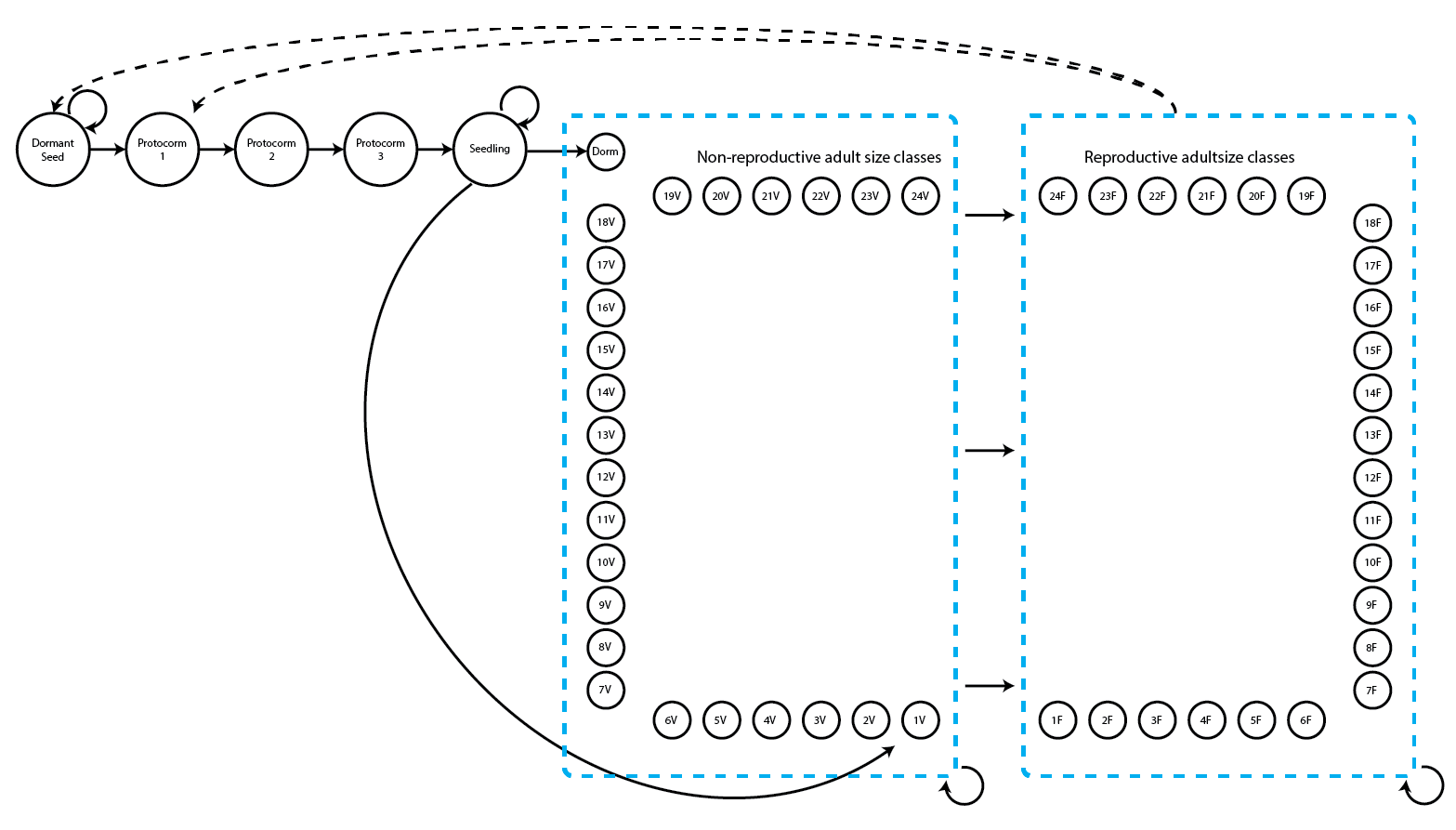
We can alter our code to account for this subtle but nonetheless major change with just two steps. First, we will add stage groups to our stage frame. We will assign the dormant seed stage, three protocorm stages, and seedling stage to a juvenile stage group; the dormant and non-reproductive adult stages to an adult stage group; and the reproductive adult stages to a second adult stage group. This only requires adding one further vector coding these groups. Please bear in mind that stage groups must be numbered sequentially, and the first stage group must be group 0.
groupvec <- c(rep(0, 5), rep(1, 25), rep(2, 24))
cypframe_fb_group <- sf_create(sizes = sizevector, stagenames = stagevector,
repstatus = repvector, obsstatus = obsvector, matstatus = matvector,
propstatus = propvector, immstatus = immvector, indataset = indataset,
group = groupvec, comments = comments)
cypframe_fb_group
> stage size size_b size_c min_age max_age repstatus obsstatus propstatus
> 1 SD 0 NA NA NA NA 0 0 1
> 2 P1 0 NA NA NA NA 0 0 0
> 3 P2 0 NA NA NA NA 0 0 0
> 4 P3 0 NA NA NA NA 0 0 0
> 5 SL 0 NA NA NA NA 0 0 0
> 6 Dorm 0 NA NA NA NA 0 0 0
> 7 1V 1 NA NA NA NA 0 1 0
> 8 2V 2 NA NA NA NA 0 1 0
> 9 3V 3 NA NA NA NA 0 1 0
> 10 4V 4 NA NA NA NA 0 1 0
> 11 5V 5 NA NA NA NA 0 1 0
> 12 6V 6 NA NA NA NA 0 1 0
> 13 7V 7 NA NA NA NA 0 1 0
> 14 8V 8 NA NA NA NA 0 1 0
> 15 9V 9 NA NA NA NA 0 1 0
> 16 10V 10 NA NA NA NA 0 1 0
> 17 11V 11 NA NA NA NA 0 1 0
> 18 12V 12 NA NA NA NA 0 1 0
> 19 13V 13 NA NA NA NA 0 1 0
> 20 14V 14 NA NA NA NA 0 1 0
> 21 15V 15 NA NA NA NA 0 1 0
> 22 16V 16 NA NA NA NA 0 1 0
> 23 17V 17 NA NA NA NA 0 1 0
> 24 18V 18 NA NA NA NA 0 1 0
> 25 19V 19 NA NA NA NA 0 1 0
> 26 20V 20 NA NA NA NA 0 1 0
> 27 21V 21 NA NA NA NA 0 1 0
> 28 22V 22 NA NA NA NA 0 1 0
> 29 23V 23 NA NA NA NA 0 1 0
> 30 24V 24 NA NA NA NA 0 1 0
> 31 1F 1 NA NA NA NA 1 1 0
> 32 2F 2 NA NA NA NA 1 1 0
> 33 3F 3 NA NA NA NA 1 1 0
> 34 4F 4 NA NA NA NA 1 1 0
> immstatus matstatus indataset binhalfwidth_raw sizebin_min sizebin_max
> 1 0 0 0 0.5 -0.5 0.5
> 2 1 0 0 0.5 -0.5 0.5
> 3 1 0 0 0.5 -0.5 0.5
> 4 1 0 0 0.5 -0.5 0.5
> 5 1 0 0 0.5 -0.5 0.5
> 6 0 1 1 0.5 -0.5 0.5
> 7 0 1 1 0.5 0.5 1.5
> 8 0 1 1 0.5 1.5 2.5
> 9 0 1 1 0.5 2.5 3.5
> 10 0 1 1 0.5 3.5 4.5
> 11 0 1 1 0.5 4.5 5.5
> 12 0 1 1 0.5 5.5 6.5
> 13 0 1 1 0.5 6.5 7.5
> 14 0 1 1 0.5 7.5 8.5
> 15 0 1 1 0.5 8.5 9.5
> 16 0 1 1 0.5 9.5 10.5
> 17 0 1 1 0.5 10.5 11.5
> 18 0 1 1 0.5 11.5 12.5
> 19 0 1 1 0.5 12.5 13.5
> 20 0 1 1 0.5 13.5 14.5
> 21 0 1 1 0.5 14.5 15.5
> 22 0 1 1 0.5 15.5 16.5
> 23 0 1 1 0.5 16.5 17.5
> 24 0 1 1 0.5 17.5 18.5
> 25 0 1 1 0.5 18.5 19.5
> 26 0 1 1 0.5 19.5 20.5
> 27 0 1 1 0.5 20.5 21.5
> 28 0 1 1 0.5 21.5 22.5
> 29 0 1 1 0.5 22.5 23.5
> 30 0 1 1 0.5 23.5 24.5
> 31 0 1 1 0.5 0.5 1.5
> 32 0 1 1 0.5 1.5 2.5
> 33 0 1 1 0.5 2.5 3.5
> 34 0 1 1 0.5 3.5 4.5
> sizebin_center sizebin_width binhalfwidthb_raw sizebinb_min sizebinb_max
> 1 0 1 NA NA NA
> 2 0 1 NA NA NA
> 3 0 1 NA NA NA
> 4 0 1 NA NA NA
> 5 0 1 NA NA NA
> 6 0 1 NA NA NA
> 7 1 1 NA NA NA
> 8 2 1 NA NA NA
> 9 3 1 NA NA NA
> 10 4 1 NA NA NA
> 11 5 1 NA NA NA
> 12 6 1 NA NA NA
> 13 7 1 NA NA NA
> 14 8 1 NA NA NA
> 15 9 1 NA NA NA
> 16 10 1 NA NA NA
> 17 11 1 NA NA NA
> 18 12 1 NA NA NA
> 19 13 1 NA NA NA
> 20 14 1 NA NA NA
> 21 15 1 NA NA NA
> 22 16 1 NA NA NA
> 23 17 1 NA NA NA
> 24 18 1 NA NA NA
> 25 19 1 NA NA NA
> 26 20 1 NA NA NA
> 27 21 1 NA NA NA
> 28 22 1 NA NA NA
> 29 23 1 NA NA NA
> 30 24 1 NA NA NA
> 31 1 1 NA NA NA
> 32 2 1 NA NA NA
> 33 3 1 NA NA NA
> 34 4 1 NA NA NA
> sizebinb_center sizebinb_width binhalfwidthc_raw sizebinc_min sizebinc_max
> 1 NA NA NA NA NA
> 2 NA NA NA NA NA
> 3 NA NA NA NA NA
> 4 NA NA NA NA NA
> 5 NA NA NA NA NA
> 6 NA NA NA NA NA
> 7 NA NA NA NA NA
> 8 NA NA NA NA NA
> 9 NA NA NA NA NA
> 10 NA NA NA NA NA
> 11 NA NA NA NA NA
> 12 NA NA NA NA NA
> 13 NA NA NA NA NA
> 14 NA NA NA NA NA
> 15 NA NA NA NA NA
> 16 NA NA NA NA NA
> 17 NA NA NA NA NA
> 18 NA NA NA NA NA
> 19 NA NA NA NA NA
> 20 NA NA NA NA NA
> 21 NA NA NA NA NA
> 22 NA NA NA NA NA
> 23 NA NA NA NA NA
> 24 NA NA NA NA NA
> 25 NA NA NA NA NA
> 26 NA NA NA NA NA
> 27 NA NA NA NA NA
> 28 NA NA NA NA NA
> 29 NA NA NA NA NA
> 30 NA NA NA NA NA
> 31 NA NA NA NA NA
> 32 NA NA NA NA NA
> 33 NA NA NA NA NA
> 34 NA NA NA NA NA
> sizebinc_center sizebinc_width group comments
> 1 NA NA 0 Dormant seed
> 2 NA NA 0 Yr1 protocorm
> 3 NA NA 0 Yr2 protocorm
> 4 NA NA 0 Yr3 protocorm
> 5 NA NA 0 Seedling
> 6 NA NA 1 Veg dorm
> 7 NA NA 1 Veg adult 1 stem
> 8 NA NA 1 Veg adult 2 stems
> 9 NA NA 1 Veg adult 3 stems
> 10 NA NA 1 Veg adult 4 stems
> 11 NA NA 1 Veg adult 5 stems
> 12 NA NA 1 Veg adult 6 stems
> 13 NA NA 1 Veg adult 7 stems
> 14 NA NA 1 Veg adult 8 stems
> 15 NA NA 1 Veg adult 9 stems
> 16 NA NA 1 Veg adult 10 stems
> 17 NA NA 1 Veg adult 11 stems
> 18 NA NA 1 Veg adult 12 stems
> 19 NA NA 1 Veg adult 13 stems
> 20 NA NA 1 Veg adult 14 stems
> 21 NA NA 1 Veg adult 15 stems
> 22 NA NA 1 Veg adult 16 stems
> 23 NA NA 1 Veg adult 17 stems
> 24 NA NA 1 Veg adult 18 stems
> 25 NA NA 1 Veg adult 19 stems
> 26 NA NA 1 Veg adult 20 stems
> 27 NA NA 1 Veg adult 21 stems
> 28 NA NA 1 Veg adult 22 stems
> 29 NA NA 1 Veg adult 23 stems
> 30 NA NA 1 Veg adult 24 stems
> 31 NA NA 2 Flo adult 1 stem
> 32 NA NA 2 Flo adult 2 stems
> 33 NA NA 2 Flo adult 3 stems
> 34 NA NA 2 Flo adult 4 stems
> [ reached 'max' / getOption("max.print") -- omitted 20 rows ]
Next, we will add an extra line to the supplement table to set transitions from group 2 to group 1 to a value of 0.0. This effectively disallows transitions back from reproductive to non-reproductive adult stages. We will do this with our ahistorical supplement table and create only ahistorical MPMs, but this may also be done with the historical supplement table to create historical MPMs.
cypsupp2_fb_group <- supplemental(stage3 = c("SD", "P1", "P2", "P3", "SL", "SL",
    "Dorm", "1V", "2V", "3V", "SD", "P1", "group1"),
  stage2 = c("SD", "SD", "P1", "P2", "P3", "SL", "SL", "SL", "SL", "SL", "rep",
    "rep", "group2"),
  eststage3 = c(NA, NA, NA, NA, NA, NA, "Dorm", "1V", "2V", "3V", NA, NA, NA),
  eststage2 = c(NA, NA, NA, NA, NA, NA, "Dorm", "Dorm", "Dorm", "Dorm", NA, NA, NA),
  givenrate = c(0.08, 0.1, 0.1, 0.1, 0.05, 0.05, NA, NA, NA, NA, NA, NA, 0.0),
  multiplier = c(NA, NA, NA, NA, NA, NA, sl_mult, sl_mult, sl_mult, sl_mult,
    0.5 * seeds_per_fruit, 0.5 * seeds_per_fruit, NA),
  type = c("S", "S", "S", "S", "S", "S", "S", "S", "S", "S", "R", "R", "S"),
  stageframe = cypframe_fb_group, historical = FALSE)
> Warning: NA values in argument multiplier will be treated as 1 values.

cypsupp2_fb_group
>    stage3 stage2 stage1 age2 eststage3 eststage2 eststage1 estage2 givenrate
> 1      SD     SD   <NA>   NA      <NA>      <NA>      <NA>      NA      0.08
> 2      P1     SD   <NA>   NA      <NA>      <NA>      <NA>      NA      0.10
> 3      P2     P1   <NA>   NA      <NA>      <NA>      <NA>      NA      0.10
> 4      P3     P2   <NA>   NA      <NA>      <NA>      <NA>      NA      0.10
> 5      SL     P3   <NA>   NA      <NA>      <NA>      <NA>      NA      0.05
> 6      SL     SL   <NA>   NA      <NA>      <NA>      <NA>      NA      0.05
> 7    Dorm     SL   <NA>   NA      Dorm      Dorm      <NA>      NA        NA
> 8      1V     SL   <NA>   NA        1V      Dorm      <NA>      NA        NA
> 9      2V     SL   <NA>   NA        2V      Dorm      <NA>      NA        NA
> 10     3V     SL   <NA>   NA        3V      Dorm      <NA>      NA        NA
> 11     SD    rep   <NA>   NA      <NA>      <NA>      <NA>      NA        NA
> 12     P1    rep   <NA>   NA      <NA>      <NA>      <NA>      NA        NA
> 13 group1 group2   <NA>   NA      <NA>      <NA>      <NA>      NA      0.00
>    offset multiplier convtype convtype_t12
> 1      NA        1.0        1            1
> 2      NA        1.0        1            1
> 3      NA        1.0        1            1
> 4      NA        1.0        1            1
> 5      NA        1.0        1            1
> 6      NA        1.0        1            1
> 7      NA        0.7        1            1
> 8      NA        0.7        1            1
> 9      NA        0.7        1            1
> 10     NA        0.7        1            1
> 11     NA     2500.0        3            1
> 12     NA     2500.0        3            1
> 13     NA        1.0        1            1
Finally, let’s create our new ahistorical MPM, and take a look at the first matrix.
cypmatrix2fp_group <- flefko2(stageframe = cypframe_fb_group, data = cypfb_v1,
  supplement = cypsupp2_fb_group, modelsuite = cypmodels2p)

cypmatrix2fp_group$A[[1]]
>       [,1] [,2] [,3] [,4]       [,5]         [,6]         [,7]         [,8]
>  [1,] 0.08  0.0  0.0 0.00 0.00000000 0.000000e+00 0.000000e+00 0.000000e+00
>  [2,] 0.10  0.0  0.0 0.00 0.00000000 0.000000e+00 0.000000e+00 0.000000e+00
>  [3,] 0.00  0.1  0.0 0.00 0.00000000 0.000000e+00 0.000000e+00 0.000000e+00
>  [4,] 0.00  0.0  0.1 0.00 0.00000000 0.000000e+00 0.000000e+00 0.000000e+00
>  [5,] 0.00  0.0  0.0 0.05 0.05000000 0.000000e+00 0.000000e+00 0.000000e+00
>  [6,] 0.00  0.0  0.0 0.00 0.03291481 4.702115e-02 3.686950e-02 2.809355e-02
>  [7,] 0.00  0.0  0.0 0.00 0.16278266 2.325467e-01 2.383836e-01 2.359753e-01
>  [8,] 0.00  0.0  0.0 0.00 0.10351780 1.478826e-01 1.515945e-01 1.500630e-01
>  [9,] 0.00  0.0  0.0 0.00 0.06582971 9.404244e-02 9.640294e-02 9.542902e-02
> [10,] 0.00  0.0  0.0 0.00 0.00000000 5.980408e-02 6.130518e-02 6.068584e-02
> [11,] 0.00  0.0  0.0 0.00 0.00000000 3.803100e-02 3.898559e-02 3.859173e-02
> [12,] 0.00  0.0  0.0 0.00 0.00000000 2.418492e-02 2.479197e-02 2.454150e-02
> [13,] 0.00  0.0  0.0 0.00 0.00000000 1.537983e-02 1.576587e-02 1.560659e-02
> [14,] 0.00  0.0  0.0 0.00 0.00000000 9.780441e-03 1.002593e-02 9.924645e-03
> [15,] 0.00  0.0  0.0 0.00 0.00000000 6.219642e-03 6.375756e-03 6.311345e-03
> [16,] 0.00  0.0  0.0 0.00 0.00000000 3.955235e-03 4.054512e-03 4.013551e-03
> [17,] 0.00  0.0  0.0 0.00 0.00000000 2.515238e-03 2.578372e-03 2.552324e-03
> [18,] 0.00  0.0  0.0 0.00 0.00000000 1.599507e-03 1.639655e-03 1.623090e-03
>               [,9]        [,10]        [,11]        [,12]        [,13]
>  [1,] 0.000000e+00 0.000000e+00 0.000000e+00 0.000000e+00 0.000000e+00
>  [2,] 0.000000e+00 0.000000e+00 0.000000e+00 0.000000e+00 0.000000e+00
>  [3,] 0.000000e+00 0.000000e+00 0.000000e+00 0.000000e+00 0.000000e+00
>  [4,] 0.000000e+00 0.000000e+00 0.000000e+00 0.000000e+00 0.000000e+00
>  [5,] 0.000000e+00 0.000000e+00 0.000000e+00 0.000000e+00 0.000000e+00
>  [6,] 2.104751e-02 1.561422e-02 1.151723e-02 8.466545e-03 6.211278e-03
>  [7,] 2.281165e-01 2.167851e-01 2.032902e-01 1.885092e-01 1.730645e-01
>  [8,] 1.450653e-01 1.378594e-01 1.292776e-01 1.198780e-01 1.100563e-01
>  [9,] 9.225088e-02 8.766842e-02 8.221104e-02 7.623358e-02 6.998772e-02
> [10,] 5.866478e-02 5.575067e-02 5.228018e-02 4.847895e-02 4.450705e-02
> [11,] 3.730649e-02 3.545333e-02 3.324635e-02 3.082905e-02 2.830321e-02
> [12,] 2.372418e-02 2.254571e-02 2.114223e-02 1.960501e-02 1.799876e-02
> [13,] 1.508684e-02 1.433741e-02 1.344491e-02 1.246734e-02 1.144589e-02
> [14,] 9.594118e-03 9.117541e-03 8.549972e-03 7.928314e-03 7.278744e-03
> [15,] 6.101154e-03 5.798086e-03 5.437154e-03 5.041825e-03 4.628746e-03
> [16,] 3.879885e-03 3.687156e-03 3.457630e-03 3.206230e-03 2.943542e-03
> [17,] 2.467322e-03 2.344760e-03 2.198799e-03 2.038926e-03 1.871876e-03
> [18,] 1.569035e-03 1.491095e-03 1.398274e-03 1.296607e-03 1.190376e-03
>              [,14]        [,15]        [,16]        [,17]        [,18]
>  [1,] 0.000000e+00 0.000000e+00 0.000000e+00 0.000000e+00 0.000000e+00
>  [2,] 0.000000e+00 0.000000e+00 0.000000e+00 0.000000e+00 0.000000e+00
>  [3,] 0.000000e+00 0.000000e+00 0.000000e+00 0.000000e+00 0.000000e+00
>  [4,] 0.000000e+00 0.000000e+00 0.000000e+00 0.000000e+00 0.000000e+00
>  [5,] 0.000000e+00 0.000000e+00 0.000000e+00 0.000000e+00 0.000000e+00
>  [6,] 4.551060e-03 3.331976e-03 2.438204e-03 1.783578e-03 1.304415e-03
>  [7,] 1.574279e-01 1.419733e-01 1.270014e-01 1.127486e-01 9.939104e-02
>  [8,] 1.001125e-01 9.028458e-02 8.076356e-02 7.169980e-02 6.320539e-02
>  [9,] 6.366422e-02 5.741436e-02 5.135969e-02 4.559580e-02 4.019398e-02
> [10,] 4.048576e-02 3.651131e-02 3.266099e-02 2.899558e-02 2.556042e-02
> [11,] 2.574597e-02 2.321851e-02 2.076999e-02 1.843906e-02 1.625455e-02
> [12,] 1.637254e-02 1.476526e-02 1.320818e-02 1.172588e-02 1.033670e-02
> [13,] 1.041173e-02 9.389623e-03 8.399434e-03 7.456800e-03 6.573379e-03
> [14,] 6.621097e-03 5.971110e-03 5.341422e-03 4.741977e-03 4.180186e-03
> [15,] 4.210531e-03 3.797187e-03 3.396752e-03 3.015549e-03 2.658291e-03
> [16,] 2.677588e-03 2.414732e-03 2.160084e-03 1.917667e-03 1.690477e-03
> [17,] 1.702749e-03 1.535592e-03 1.373655e-03 1.219495e-03 1.075019e-03
> [18,] 1.082823e-03 9.765235e-04 8.735435e-04 7.755094e-04 6.836333e-04
>              [,19]        [,20]        [,21]        [,22]        [,23]
>  [1,] 0.000000e+00 0.000000e+00 0.000000e+00 0.000000e+00 0.000000e+00
>  [2,] 0.000000e+00 0.000000e+00 0.000000e+00 0.000000e+00 0.000000e+00
>  [3,] 0.000000e+00 0.000000e+00 0.000000e+00 0.000000e+00 0.000000e+00
>  [4,] 0.000000e+00 0.000000e+00 0.000000e+00 0.000000e+00 0.000000e+00
>  [5,] 0.000000e+00 0.000000e+00 0.000000e+00 0.000000e+00 0.000000e+00
>  [6,] 9.538315e-04 6.973975e-04 5.098657e-04 3.727414e-04 2.724849e-04
>  [7,] 8.704831e-02 7.578798e-02 6.563239e-02 5.656661e-02 4.854699e-02
>  [8,] 5.535632e-02 4.819558e-02 4.173737e-02 3.597221e-02 3.087232e-02
>  [9,] 3.520255e-02 3.064885e-02 2.654190e-02 2.287568e-02 1.963252e-02
> [10,] 2.238623e-02 1.949041e-02 1.687870e-02 1.454725e-02 1.248484e-02
> [11,] 1.423600e-02 1.239447e-02 1.073361e-02 9.250981e-03 7.939442e-03
> [12,] 9.053049e-03 7.881972e-03 6.825788e-03 5.882944e-03 5.048901e-03
> [13,] 5.757074e-03 5.012355e-03 4.340699e-03 3.741120e-03 3.210730e-03
> [14,] 3.661075e-03 3.187489e-03 2.760365e-03 2.379077e-03 2.041788e-03
> [15,] 2.328175e-03 2.027009e-03 1.755389e-03 1.512918e-03 1.298427e-03
> [16,] 1.480548e-03 1.289028e-03 1.116299e-03 9.621047e-04 8.257042e-04
> [17,] 9.415197e-04 8.197273e-04 7.098839e-04 6.118279e-04 5.250872e-04
> [18,] 5.987373e-04 5.212863e-04 4.514339e-04 3.890775e-04 3.339168e-04
>              [,24]        [,25]        [,26]        [,27]        [,28]
>  [1,] 0.000000e+00 0.000000e+00 0.000000e+00 0.000000e+00 0.000000e+00
>  [2,] 0.000000e+00 0.000000e+00 0.000000e+00 0.000000e+00 0.000000e+00
>  [3,] 0.000000e+00 0.000000e+00 0.000000e+00 0.000000e+00 0.000000e+00
>  [4,] 0.000000e+00 0.000000e+00 0.000000e+00 0.000000e+00 0.000000e+00
>  [5,] 0.000000e+00 0.000000e+00 0.000000e+00 0.000000e+00 0.000000e+00
>  [6,] 1.991889e-04 1.456059e-04 1.064355e-04 7.780170e-05 5.687068e-05
>  [7,] 4.150943e-02 3.537682e-02 3.006528e-02 2.548907e-02 2.156424e-02
>  [8,] 2.639695e-02 2.249706e-02 1.911931e-02 1.620917e-02 1.371327e-02
>  [9,] 1.678652e-02 1.430647e-02 1.215847e-02 1.030784e-02 8.720633e-03
> [10,] 1.067499e-02 9.097866e-03 7.731895e-03 6.555030e-03 5.545681e-03
> [11,] 6.788509e-03 5.785574e-03 4.916917e-03 4.168517e-03 3.526646e-03
> [12,] 4.316993e-03 3.679200e-03 3.126798e-03 2.650871e-03 2.242687e-03
> [13,] 2.745290e-03 2.339700e-03 1.988413e-03 1.685759e-03 1.426184e-03
> [14,] 1.745803e-03 1.487877e-03 1.264485e-03 1.072019e-03 9.069483e-04
> [15,] 1.110202e-03 9.461807e-04 8.041194e-04 6.817250e-04 5.767525e-04
> [16,] 7.060069e-04 6.017014e-04 5.113608e-04 4.335270e-04 3.667722e-04
> [17,] 4.489685e-04 3.826378e-04 3.251879e-04 2.756913e-04 2.332401e-04
> [18,] 2.855110e-04 2.433295e-04 2.067956e-04 1.753194e-04 1.483236e-04
>              [,29]        [,30]        [,31]        [,32]        [,33]
>  [1,] 0.000000e+00 0.000000e+00 8.130827e+02 8.130827e+02 8.130827e+02
>  [2,] 0.000000e+00 0.000000e+00 8.130827e+02 8.130827e+02 8.130827e+02
>  [3,] 0.000000e+00 0.000000e+00 0.000000e+00 0.000000e+00 0.000000e+00
>  [4,] 0.000000e+00 0.000000e+00 0.000000e+00 0.000000e+00 0.000000e+00
>  [5,] 0.000000e+00 0.000000e+00 0.000000e+00 0.000000e+00 0.000000e+00
>  [6,] 4.157051e-05 3.038649e-05 0.000000e+00 0.000000e+00 0.000000e+00
>  [7,] 1.821114e-02 1.535598e-02 0.000000e+00 0.000000e+00 0.000000e+00
>  [8,] 1.158095e-02 9.765277e-03 0.000000e+00 0.000000e+00 0.000000e+00
>  [9,] 7.364631e-03 6.209998e-03 0.000000e+00 0.000000e+00 0.000000e+00
> [10,] 4.683364e-03 3.949102e-03 0.000000e+00 0.000000e+00 0.000000e+00
> [11,] 2.978275e-03 2.511339e-03 0.000000e+00 0.000000e+00 0.000000e+00
> [12,] 1.893964e-03 1.597027e-03 0.000000e+00 0.000000e+00 0.000000e+00
> [13,] 1.204422e-03 1.015592e-03 0.000000e+00 0.000000e+00 0.000000e+00
> [14,] 7.659238e-04 6.458416e-04 0.000000e+00 0.000000e+00 0.000000e+00
> [15,] 4.870712e-04 4.107078e-04 0.000000e+00 0.000000e+00 0.000000e+00
> [16,] 3.097415e-04 2.611800e-04 0.000000e+00 0.000000e+00 0.000000e+00
> [17,] 1.969728e-04 1.660912e-04 0.000000e+00 0.000000e+00 0.000000e+00
> [18,] 1.252602e-04 1.056218e-04 0.000000e+00 0.000000e+00 0.000000e+00
>              [,34]        [,35]        [,36]        [,37]        [,38]
>  [1,] 8.130827e+02 8.130827e+02 8.130827e+02 8.130827e+02 8.130827e+02
>  [2,] 8.130827e+02 8.130827e+02 8.130827e+02 8.130827e+02 8.130827e+02
>  [3,] 0.000000e+00 0.000000e+00 0.000000e+00 0.000000e+00 0.000000e+00
>  [4,] 0.000000e+00 0.000000e+00 0.000000e+00 0.000000e+00 0.000000e+00
>  [5,] 0.000000e+00 0.000000e+00 0.000000e+00 0.000000e+00 0.000000e+00
>  [6,] 0.000000e+00 0.000000e+00 0.000000e+00 0.000000e+00 0.000000e+00
>  [7,] 0.000000e+00 0.000000e+00 0.000000e+00 0.000000e+00 0.000000e+00
>  [8,] 0.000000e+00 0.000000e+00 0.000000e+00 0.000000e+00 0.000000e+00
>  [9,] 0.000000e+00 0.000000e+00 0.000000e+00 0.000000e+00 0.000000e+00
> [10,] 0.000000e+00 0.000000e+00 0.000000e+00 0.000000e+00 0.000000e+00
> [11,] 0.000000e+00 0.000000e+00 0.000000e+00 0.000000e+00 0.000000e+00
> [12,] 0.000000e+00 0.000000e+00 0.000000e+00 0.000000e+00 0.000000e+00
> [13,] 0.000000e+00 0.000000e+00 0.000000e+00 0.000000e+00 0.000000e+00
> [14,] 0.000000e+00 0.000000e+00 0.000000e+00 0.000000e+00 0.000000e+00
> [15,] 0.000000e+00 0.000000e+00 0.000000e+00 0.000000e+00 0.000000e+00
> [16,] 0.000000e+00 0.000000e+00 0.000000e+00 0.000000e+00 0.000000e+00
> [17,] 0.000000e+00 0.000000e+00 0.000000e+00 0.000000e+00 0.000000e+00
> [18,] 0.000000e+00 0.000000e+00 0.000000e+00 0.000000e+00 0.000000e+00
>              [,39]        [,40]        [,41]        [,42]        [,43]
>  [1,] 8.130827e+02 8.130827e+02 8.130827e+02 8.130827e+02 8.130827e+02
>  [2,] 8.130827e+02 8.130827e+02 8.130827e+02 8.130827e+02 8.130827e+02
>  [3,] 0.000000e+00 0.000000e+00 0.000000e+00 0.000000e+00 0.000000e+00
>  [4,] 0.000000e+00 0.000000e+00 0.000000e+00 0.000000e+00 0.000000e+00
>  [5,] 0.000000e+00 0.000000e+00 0.000000e+00 0.000000e+00 0.000000e+00
>  [6,] 0.000000e+00 0.000000e+00 0.000000e+00 0.000000e+00 0.000000e+00
>  [7,] 0.000000e+00 0.000000e+00 0.000000e+00 0.000000e+00 0.000000e+00
>  [8,] 0.000000e+00 0.000000e+00 0.000000e+00 0.000000e+00 0.000000e+00
>  [9,] 0.000000e+00 0.000000e+00 0.000000e+00 0.000000e+00 0.000000e+00
> [10,] 0.000000e+00 0.000000e+00 0.000000e+00 0.000000e+00 0.000000e+00
> [11,] 0.000000e+00 0.000000e+00 0.000000e+00 0.000000e+00 0.000000e+00
> [12,] 0.000000e+00 0.000000e+00 0.000000e+00 0.000000e+00 0.000000e+00
> [13,] 0.000000e+00 0.000000e+00 0.000000e+00 0.000000e+00 0.000000e+00
> [14,] 0.000000e+00 0.000000e+00 0.000000e+00 0.000000e+00 0.000000e+00
> [15,] 0.000000e+00 0.000000e+00 0.000000e+00 0.000000e+00 0.000000e+00
> [16,] 0.000000e+00 0.000000e+00 0.000000e+00 0.000000e+00 0.000000e+00
> [17,] 0.000000e+00 0.000000e+00 0.000000e+00 0.000000e+00 0.000000e+00
> [18,] 0.000000e+00 0.000000e+00 0.000000e+00 0.000000e+00 0.000000e+00
>              [,44]        [,45]        [,46]        [,47]        [,48]
>  [1,] 8.130827e+02 8.130827e+02 8.130827e+02 8.130827e+02 8.130827e+02
>  [2,] 8.130827e+02 8.130827e+02 8.130827e+02 8.130827e+02 8.130827e+02
>  [3,] 0.000000e+00 0.000000e+00 0.000000e+00 0.000000e+00 0.000000e+00
>  [4,] 0.000000e+00 0.000000e+00 0.000000e+00 0.000000e+00 0.000000e+00
>  [5,] 0.000000e+00 0.000000e+00 0.000000e+00 0.000000e+00 0.000000e+00
>  [6,] 0.000000e+00 0.000000e+00 0.000000e+00 0.000000e+00 0.000000e+00
>  [7,] 0.000000e+00 0.000000e+00 0.000000e+00 0.000000e+00 0.000000e+00
>  [8,] 0.000000e+00 0.000000e+00 0.000000e+00 0.000000e+00 0.000000e+00
>  [9,] 0.000000e+00 0.000000e+00 0.000000e+00 0.000000e+00 0.000000e+00
> [10,] 0.000000e+00 0.000000e+00 0.000000e+00 0.000000e+00 0.000000e+00
> [11,] 0.000000e+00 0.000000e+00 0.000000e+00 0.000000e+00 0.000000e+00
> [12,] 0.000000e+00 0.000000e+00 0.000000e+00 0.000000e+00 0.000000e+00
> [13,] 0.000000e+00 0.000000e+00 0.000000e+00 0.000000e+00 0.000000e+00
> [14,] 0.000000e+00 0.000000e+00 0.000000e+00 0.000000e+00 0.000000e+00
> [15,] 0.000000e+00 0.000000e+00 0.000000e+00 0.000000e+00 0.000000e+00
> [16,] 0.000000e+00 0.000000e+00 0.000000e+00 0.000000e+00 0.000000e+00
> [17,] 0.000000e+00 0.000000e+00 0.000000e+00 0.000000e+00 0.000000e+00
> [18,] 0.000000e+00 0.000000e+00 0.000000e+00 0.000000e+00 0.000000e+00
>              [,49]        [,50]        [,51]        [,52]        [,53]
>  [1,] 8.130827e+02 8.130827e+02 8.130827e+02 8.130827e+02 8.130827e+02
>  [2,] 8.130827e+02 8.130827e+02 8.130827e+02 8.130827e+02 8.130827e+02
>  [3,] 0.000000e+00 0.000000e+00 0.000000e+00 0.000000e+00 0.000000e+00
>  [4,] 0.000000e+00 0.000000e+00 0.000000e+00 0.000000e+00 0.000000e+00
>  [5,] 0.000000e+00 0.000000e+00 0.000000e+00 0.000000e+00 0.000000e+00
>  [6,] 0.000000e+00 0.000000e+00 0.000000e+00 0.000000e+00 0.000000e+00
>  [7,] 0.000000e+00 0.000000e+00 0.000000e+00 0.000000e+00 0.000000e+00
>  [8,] 0.000000e+00 0.000000e+00 0.000000e+00 0.000000e+00 0.000000e+00
>  [9,] 0.000000e+00 0.000000e+00 0.000000e+00 0.000000e+00 0.000000e+00
> [10,] 0.000000e+00 0.000000e+00 0.000000e+00 0.000000e+00 0.000000e+00
> [11,] 0.000000e+00 0.000000e+00 0.000000e+00 0.000000e+00 0.000000e+00
> [12,] 0.000000e+00 0.000000e+00 0.000000e+00 0.000000e+00 0.000000e+00
> [13,] 0.000000e+00 0.000000e+00 0.000000e+00 0.000000e+00 0.000000e+00
> [14,] 0.000000e+00 0.000000e+00 0.000000e+00 0.000000e+00 0.000000e+00
> [15,] 0.000000e+00 0.000000e+00 0.000000e+00 0.000000e+00 0.000000e+00
> [16,] 0.000000e+00 0.000000e+00 0.000000e+00 0.000000e+00 0.000000e+00
> [17,] 0.000000e+00 0.000000e+00 0.000000e+00 0.000000e+00 0.000000e+00
> [18,] 0.000000e+00 0.000000e+00 0.000000e+00 0.000000e+00 0.000000e+00
>              [,54]
>  [1,] 8.130827e+02
>  [2,] 8.130827e+02
>  [3,] 0.000000e+00
>  [4,] 0.000000e+00
>  [5,] 0.000000e+00
>  [6,] 0.000000e+00
>  [7,] 0.000000e+00
>  [8,] 0.000000e+00
>  [9,] 0.000000e+00
> [10,] 0.000000e+00
> [11,] 0.000000e+00
> [12,] 0.000000e+00
> [13,] 0.000000e+00
> [14,] 0.000000e+00
> [15,] 0.000000e+00
> [16,] 0.000000e+00
> [17,] 0.000000e+00
> [18,] 0.000000e+00
>  [ reached 'max' / getOption("max.print") -- omitted 36 rows ]
Notice that a large portion of the entries are now zeros. We can also explore a summary of this MPM to see the reduction in estimated elements (the summary() function only counts elements as estimated if they are non-zero), particularly in comparison to the original ahistorical MPM.
summary(cypmatrix2fp_group)
>
> This ahistorical lefkoMat object contains 15 matrices.
>
> Each matrix is square with 54 rows and columns, and a total of 2916 elements.
> A total of 27165 survival transitions were estimated, with 1811 per matrix.
> A total of 720 fecundity transitions were estimated, with 48 per matrix.
> This lefkoMat object covers 1 population, 3 patches, and 5 time steps.
>
> The dataset contains a total of 74 unique individuals and 320 unique transitions.
>
> Vital rate modeling quality control:
>
> Survival estimated with 74 individuals and 320 individual transitions.
> Observation estimated with 70 individuals and 303 individual transitions.
> Primary size estimated with 70 individuals and 288 individual transitions.
> Secondary size transition not estimated.
> Tertiary size transition not estimated.
> Reproductive status estimated with 70 individuals and 288 individual transitions.
> Fecundity estimated with 51 individuals and 118 individual transitions.
> Juvenile survival not estimated.
> Juvenile observation probability not estimated.
> Juvenile primary size transition not estimated.
> Juvenile secondary size transition not estimated.
> Juvenile tertiary size transition not estimated.
> Juvenile reproduction probability not estimated.
> Juvenile maturity transition probability not estimated.
>
> Survival probability sum check (each matrix represented by column in order):
>          [,1]  [,2]  [,3]  [,4]  [,5]  [,6]  [,7]  [,8]  [,9] [,10] [,11] [,12]
> Min.    0.050 0.050 0.050 0.050 0.050 0.050 0.050 0.050 0.050 0.050 0.050 0.050
> 1st Qu. 0.879 0.743 0.802 0.867 0.927 0.840 0.670 0.741 0.824 0.900 0.888 0.786
> Median  0.979 0.956 0.965 0.978 0.988 0.971 0.940 0.956 0.969 0.983 0.981 0.964
> Mean    0.865 0.819 0.838 0.858 0.887 0.850 0.796 0.818 0.843 0.877 0.873 0.832
> 3rd Qu. 1.000 1.000 1.000 1.000 1.000 1.000 1.000 1.000 1.000 1.000 1.000 1.000
> Max.    1.000 1.000 1.000 1.000 1.000 1.000 1.000 1.000 1.000 1.000 1.000 1.000
>         [,13] [,14] [,15]
> Min.    0.050 0.050 0.050
> 1st Qu. 0.838 0.885 0.936
> Median  0.971 0.981 0.990
> Mean    0.849 0.865 0.891
> 3rd Qu. 1.000 1.000 1.000
> Max.    1.000 1.000 1.000
>
>
> All matrices have no stage discontinuities.
summary(cypmatrix2fp)
>
> This ahistorical lefkoMat object contains 15 matrices.
>
> Each matrix is square with 54 rows and columns, and a total of 2916 elements.
> A total of 36165 survival transitions were estimated, with 2411 per matrix.
> A total of 720 fecundity transitions were estimated, with 48 per matrix.
> This lefkoMat object covers 1 population, 3 patches, and 5 time steps.
>
> The dataset contains a total of 74 unique individuals and 320 unique transitions.
>
> Vital rate modeling quality control:
>
> Survival estimated with 74 individuals and 320 individual transitions.
> Observation estimated with 70 individuals and 303 individual transitions.
> Primary size estimated with 70 individuals and 288 individual transitions.
> Secondary size transition not estimated.
> Tertiary size transition not estimated.
> Reproductive status estimated with 70 individuals and 288 individual transitions.
> Fecundity estimated with 51 individuals and 118 individual transitions.
> Juvenile survival not estimated.
> Juvenile observation probability not estimated.
> Juvenile primary size transition not estimated.
> Juvenile secondary size transition not estimated.
> Juvenile tertiary size transition not estimated.
> Juvenile reproduction probability not estimated.
> Juvenile maturity transition probability not estimated.
>
> Survival probability sum check (each matrix represented by column in order):
>          [,1]  [,2]  [,3]  [,4]  [,5]  [,6]  [,7]  [,8]  [,9] [,10] [,11] [,12]
> Min.    0.050 0.050 0.050 0.050 0.050 0.050 0.050 0.050 0.050 0.050 0.050 0.050
> 1st Qu. 0.991 0.991 0.991 0.991 0.991 0.991 0.991 0.991 0.991 0.991 0.991 0.991
> Median  1.000 1.000 1.000 1.000 1.000 1.000 1.000 1.000 1.000 1.000 1.000 1.000
> Mean    0.916 0.917 0.917 0.917 0.914 0.916 0.917 0.917 0.917 0.914 0.914 0.916
> 3rd Qu. 1.000 1.000 1.000 1.000 1.000 1.000 1.000 1.000 1.000 1.000 1.000 1.000
> Max.    1.000 1.000 1.000 1.000 1.000 1.000 1.000 1.000 1.000 1.000 1.000 1.000
>         [,13] [,14] [,15]
> Min.    0.050 0.050 0.050
> 1st Qu. 0.991 0.991 0.991
> Median  1.000 1.000 1.000
> Mean    0.916 0.916 0.913
> 3rd Qu. 1.000 1.000 1.000
> Max.    1.000 1.000 1.000
>
>
> All matrices have no stage discontinuities.
We can see in the output that there are 600 fewer non-zero survival terms per matrix in our new ahistorical MPM. This is because we have eliminated the return transitions from the reproductive to the non-reproductive stages. Let’s take a look at matrix images of the first \(\mathbf{A}\) matrix in the original MPM and the stage-group MPM to get a better sense of where the non-zero elements are. In the second matrix, we should see the top-right quadrant below fecundity zeroed out.
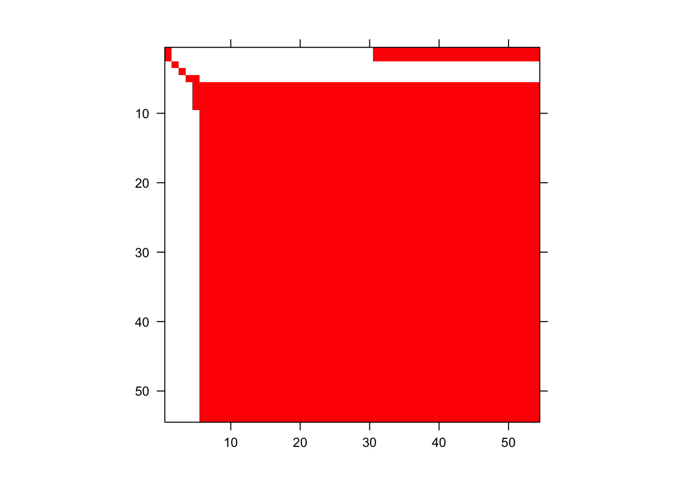
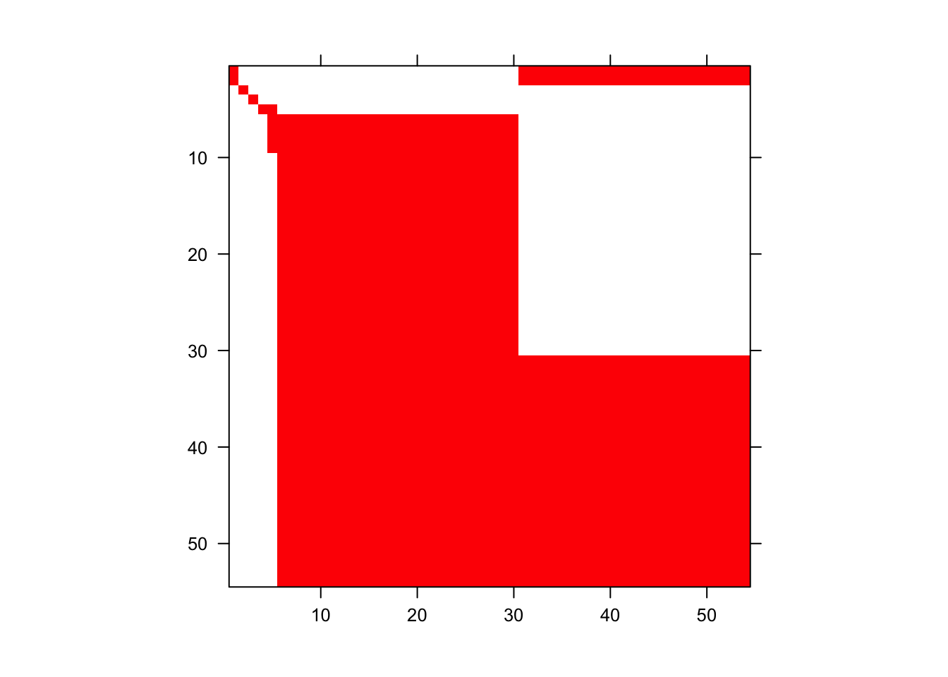
One important note here is that we used stage groups in this instance only to provide a convenient means of setting values later in the MPM itself. If we had wanted to test the impact of stage group on vital rates, then we would have needed to run function modelsearch() with option test.group = TRUE.
Using stage groups provides a great deal of power in structuring your MPMs. Now let’s move on to the use of manually estimated vital rate models in function-based MPMs.
5.7 Annual and individual covariates
Users may at times wish to develop MPMs conditioned on extra variables, including annual environmental variables such as Spring precipitation, or individual state variables such as frailty indices. Package lefko3 can handle this easily with the modelsearch() function combined with the various function-based matrix estimators. In fact, up to three individual covariates and three annual covariates can be used.
For our first example, let’s continue using the Cypripedium dataset with the life history model diagrammed in figure 5.1. We will see how total annual precipitation affects our vital rates, and use the resulting vital rates to create a new function-based MPM. The easiest way to accomplish this is to build a vector of the annual values for the covariates we have in mind, and then load them into modelsearch using the annucov series of arguments. For a single covariate, we would used only annucova combined with test.annucova = TRUE. Additional covariates can be added with annucovb and annucovc. Note that the length of the annual covariate vector must be equal to the number of years in time t in the dataset, meaning that the final year of the dataset should not be included.
precip <- c(92.2, 57.6, 96.0, 109.8, 111.9)

cypmodels2_anna <- modelsearch(cypfb_v1, historical = FALSE, approach = "mixed",
  vitalrates = c("surv", "obs", "size", "repst", "fec"),
  sizedist = "negbin", size.trunc = TRUE, fecdist = "poisson", fec.zero = TRUE,
  suite = "main", size = c("size3added", "size2added", "size1added"),
  annucova = precip, test.annucova = TRUE, quiet = "partial")
And now the summary.
summary(cypmodels2_anna)
> This LefkoMod object includes 5 linear models.
> Best-fit model criterion used: aicc&k
>
>
>
> Survival model:
> Generalized linear mixed model fit by maximum likelihood (Laplace
>   Approximation) [glmerMod]
>  Family: binomial  ( logit )
> Formula: alive3 ~ annucova2 + (1 | year2) + (1 | individ)
>    Data: surv.data
>       AIC       BIC    logLik -2*log(L)  df.resid
>  102.9757  118.0490  -47.4878   94.9757       316
> Random effects:
>  Groups  Name        Std.Dev.
>  individ (Intercept) 1197.97
>  year2   (Intercept)   89.74
> Number of obs: 320, groups:  individ, 74; year2, 5
> Fixed Effects:
> (Intercept)    annucova2
>      271.32        -2.19
> optimizer (Nelder_Mead) convergence code: 0 (OK) ; 0 optimizer warnings; 2 lme4 warnings
>
>
>
> Observation model:
> Generalized linear mixed model fit by maximum likelihood (Laplace
>   Approximation) [glmerMod]
>  Family: binomial  ( logit )
> Formula: obsstatus3 ~ size2added + (1 | year2) + (1 | individ)
>    Data: obs.data
>       AIC       BIC    logLik -2*log(L)  df.resid
>  118.2567  133.1117  -55.1284  110.2567       299
> Random effects:
>  Groups  Name        Std.Dev.
>  individ (Intercept) 1.078e-05
>  year2   (Intercept) 8.776e-01
> Number of obs: 303, groups:  individ, 70; year2, 5
> Fixed Effects:
> (Intercept)   size2added
>      2.4904       0.3134
> optimizer (Nelder_Mead) convergence code: 0 (OK) ; 0 optimizer warnings; 1 lme4 warnings
>
>
>
> Size model:
> Formula:          size3added ~ (1 | year2) + (1 | individ)
> Data: size.data
>       AIC       BIC    logLik -2*log(L)  df.resid
> 1008.2764 1022.9282 -500.1382 1000.2764       284
> Random-effects (co)variances:
>
> Conditional model:
>  Groups  Name        Std.Dev.
>  year2   (Intercept) 0.1109
>  individ (Intercept) 1.0561
>
> Number of obs: 288 / Conditional model: year2, 5; individ, 70
>
> Dispersion parameter for truncated_nbinom2 family (): 1.99e+07
>
> Fixed Effects:
>
> Conditional model:
> (Intercept)
>      0.5761
>
>
>
> Secondary size model:
> [1] 1
>
>
>
> Tertiary size model:
> [1] 1
>
>
>
> Reproductive status model:
> Generalized linear mixed model fit by maximum likelihood (Laplace
>   Approximation) [glmerMod]
>  Family: binomial  ( logit )
> Formula: repstatus3 ~ annucova2 + repstatus2 + size2added + (1 | year2) +
>     (1 | individ)
>    Data: repst.data
>       AIC       BIC    logLik -2*log(L)  df.resid
>  330.0418  352.0196 -159.0209  318.0418       282
> Random effects:
>  Groups  Name        Std.Dev.
>  individ (Intercept) 0.0002695
>  year2   (Intercept) 0.2479120
> Number of obs: 288, groups:  individ, 70; year2, 5
> Fixed Effects:
> (Intercept)    annucova2   repstatus2   size2added
>    -4.23766      0.02954      1.71091      0.17187
>
>
>
> Fecundity model:
> Formula:          feca2 ~ annucova2 + size2added + (1 | year2) + (1 | individ)
> Zero inflation:         ~size2added + (1 | year2) + (1 | individ)
> Data: fec.data
>       AIC       BIC    logLik -2*log(L)  df.resid
>  245.4867  270.4229 -113.7434  227.4867       109
> Random-effects (co)variances:
>
> Conditional model:
>  Groups  Name        Std.Dev.
>  year2   (Intercept) 0.2517
>  individ (Intercept) 0.1927
>
> Zero-inflation model:
>  Groups  Name        Std.Dev.
>  year2   (Intercept) 2.072e-04
>  individ (Intercept) 3.951e-08
>
> Number of obs: 118 / Conditional model: year2, 5; individ, 51 / Zero-inflation model: year2, 5; individ, 51
>
> Fixed Effects:
>
> Conditional model:
> (Intercept)    annucova2   size2added
>     1.68997     -0.02397      0.06174
>
> Zero-inflation model:
> (Intercept)   size2added
>       3.927       -1.618
>
>
> Juvenile survival model:
> [1] 1
>
>
>
> Juvenile observation model:
> [1] 1
>
>
>
> Juvenile size model:
> [1] 1
>
>
>
> Juvenile secondary size model:
> [1] 1
>
>
>
> Juvenile tertiary size model:
> [1] 1
>
>
>
> Juvenile reproduction model:
> [1] 1
>
>
>
> Juvenile maturity model:
> [1] 1
>
>
>
>
>
> Number of models in survival table: 7
>
> Number of models in observation table: 8
>
> Number of models in size table: 8
>
> Number of models in secondary size table: 1
>
> Number of models in tertiary size table: 1
>
> Number of models in reproduction status table: 8
>
> Number of models in fecundity table: 64
>
> Number of models in juvenile survival table: 1
>
> Number of models in juvenile observation table: 1
>
> Number of models in juvenile size table: 1
>
> Number of models in juvenile secondary size table: 1
>
> Number of models in juvenile tertiary size table: 1
>
> Number of models in juvenile reproduction table: 1
>
> Number of models in juvenile maturity table: 1
>
>
>
>
>
> General model parameter names (column 1), and
> specific names used in these models (column 2):
>                       parameter_names mainparams
> 1                              time t      year2
> 2                          individual    individ
> 3                               patch      patch
> 4                   alive in time t+1      surv3
> 5                observed in time t+1       obs3
> 6                   sizea in time t+1      size3
> 7                   sizeb in time t+1     sizeb3
> 8                   sizec in time t+1     sizec3
> 9     reproductive status in time t+1     repst3
> 10              fecundity in time t+1       fec3
> 11                fecundity in time t       fec2
> 12                    sizea in time t      size2
> 13                  sizea in time t-1      size1
> 14                    sizeb in time t     sizeb2
> 15                  sizeb in time t-1     sizeb1
> 16                    sizec in time t     sizec2
> 17                  sizec in time t-1     sizec1
> 18      reproductive status in time t     repst2
> 19    reproductive status in time t-1     repst1
> 20        maturity status in time t+1     matst3
> 21          maturity status in time t     matst2
> 22                      age in time t        age
> 23                  density in time t    density
> 24   individual covariate a in time t   indcova2
> 25 individual covariate a in time t-1   indcova1
> 26   individual covariate b in time t   indcovb2
> 27 individual covariate b in time t-1   indcovb1
> 28   individual covariate c in time t   indcovc2
> 29 individual covariate c in time t-1   indcovc1
> 30              stage group in time t     group2
> 31            stage group in time t-1     group1
> 32       annual covariate a in time t  annucova2
> 33     annual covariate a in time t-1  annucova1
> 34       annual covariate b in time t  annucovb2
> 35     annual covariate b in time t-1  annucovb1
> 36       annual covariate c in time t  annucovc2
> 37     annual covariate c in time t-1  annucovc1
>
>
>
>
>
> Quality control:
>
> Survival model estimated with 74 individuals and 320 individual transitions.
> Survival model accuracy is 1.
> Observation status model estimated with 70 individuals and 303 individual transitions.
> Observation status model accuracy is 0.95.
> Primary size model estimated with 70 individuals and 288 individual transitions.
> Primary size model R-squared is 0.822.
> Secondary size model not estimated.
> Tertiary size model not estimated.
> Reproductive status model estimated with 70 individuals and 288 individual transitions.
> Reproductive status model accuracy is 0.719.
> Fecundity model estimated with 51 individuals and 118 individual transitions.
> Fecundity model R-squared is 0.524.
> Juvenile survival model not estimated.
> Juvenile observation status model not estimated.
> Juvenile primary size model not estimated.
> Juvenile secondary size model not estimated.
> Juvenile tertiary size model not estimated.
> Juvenile reproductive status model not estimated.
> Juvenile maturity status model not estimated.
We see that annual precipitation is a fixed term in the models for survival, reproductive status, and fecundity.
Let’s now consider a more general case - the individual covariate. We might have data on an extra state variable for each individual at each time, contained in the original dataset. Since we do not have such a term in the cypdata dataset, let’s pretend that we actually added annual precipitation into that original dataset, as below.
cypdata_env <- cypdata
cypdata_env$prec.04 <- 92.2
cypdata_env$prec.05 <- 57.6
cypdata_env$prec.06 <- 96.0
cypdata_env$prec.07 <- 109.8
cypdata_env$prec.08 <- 111.9
cypdata_env$prec.09 <- 106.8

summary(cypdata_env)
>     plantid       patch        X               Y              censor
>  Min.   : 164.0   A:23   Min.   : 46.5   Min.   :-28.00   Min.   :1
>  1st Qu.: 265.0   B:35   1st Qu.: 60.1   1st Qu.: 22.50   1st Qu.:1
>  Median : 455.0   C:19   Median : 91.4   Median : 75.60   Median :1
>  Mean   : 669.1          Mean   : 92.9   Mean   : 55.54   Mean   :1
>  3rd Qu.: 829.0          3rd Qu.:142.2   3rd Qu.: 80.10   3rd Qu.:1
>  Max.   :1560.0          Max.   :173.0   Max.   :142.40   Max.   :1
>
>     Inf2.04       Inf.04           Veg.04           Pod.04       Inf2.05
>  Min.   :0    Min.   :0.0000   Min.   : 0.000   Min.   :0.0   Min.   :0.00000
>  1st Qu.:0    1st Qu.:0.0000   1st Qu.: 1.000   1st Qu.:0.0   1st Qu.:0.00000
>  Median :0    Median :0.0000   Median : 2.000   Median :0.0   Median :0.00000
>  Mean   :0    Mean   :0.6923   Mean   : 2.923   Mean   :0.2   Mean   :0.04478
>  3rd Qu.:0    3rd Qu.:1.0000   3rd Qu.: 4.000   3rd Qu.:0.0   3rd Qu.:0.00000
>  Max.   :0    Max.   :8.0000   Max.   :12.000   Max.   :3.0   Max.   :1.00000
>  NA's   :12   NA's   :12       NA's   :12       NA's   :12    NA's   :10
>      Inf.05           Veg.05          Pod.05          Inf2.06
>  Min.   : 0.000   Min.   :0.000   Min.   :0.0000   Min.   :0
>  1st Qu.: 0.000   1st Qu.:1.000   1st Qu.:0.0000   1st Qu.:0
>  Median : 0.000   Median :1.000   Median :0.0000   Median :0
>  Mean   : 1.537   Mean   :2.134   Mean   :0.6567   Mean   :0
>  3rd Qu.: 2.000   3rd Qu.:3.000   3rd Qu.:1.0000   3rd Qu.:0
>  Max.   :18.000   Max.   :9.000   Max.   :7.0000   Max.   :0
>  NA's   :10       NA's   :10      NA's   :10       NA's   :16
>      Inf.06            Veg.06           Pod.06       Inf2.07
>  Min.   : 0.0000   Min.   : 0.000   Min.   :0.0000   Mode:logical
>  1st Qu.: 0.0000   1st Qu.: 1.000   1st Qu.:0.0000   NA's:77
>  Median : 0.0000   Median : 2.000   Median :0.0000
>  Mean   : 0.9016   Mean   : 2.213   Mean   :0.3934
>  3rd Qu.: 1.0000   3rd Qu.: 3.000   3rd Qu.:0.0000
>  Max.   :18.0000   Max.   :13.000   Max.   :4.0000
>  NA's   :16        NA's   :16       NA's   :16
>      Inf.07           Veg.07           Pod.07          Inf2.08
>  Min.   :0.0000   Min.   : 0.000   Min.   :0.0000   Min.   :0
>  1st Qu.:0.0000   1st Qu.: 1.000   1st Qu.:0.0000   1st Qu.:0
>  Median :0.0000   Median : 2.000   Median :0.0000   Median :0
>  Mean   :0.6271   Mean   : 2.627   Mean   :0.0678   Mean   :0
>  3rd Qu.:1.0000   3rd Qu.: 4.000   3rd Qu.:0.0000   3rd Qu.:0
>  Max.   :7.0000   Max.   :13.000   Max.   :1.0000   Max.   :0
>  NA's   :18       NA's   :18       NA's   :18       NA's   :24
>      Inf.08            Veg.08          Pod.08          Inf2.09
>  Min.   : 0.0000   Min.   : 0.00   Min.   :0.0000   Min.   :0
>  1st Qu.: 0.0000   1st Qu.: 1.00   1st Qu.:0.0000   1st Qu.:0
>  Median : 0.0000   Median : 2.00   Median :0.0000   Median :0
>  Mean   : 0.8868   Mean   : 2.83   Mean   :0.1509   Mean   :0
>  3rd Qu.: 1.0000   3rd Qu.: 4.00   3rd Qu.:0.0000   3rd Qu.:0
>  Max.   :11.0000   Max.   :13.00   Max.   :2.0000   Max.   :0
>  NA's   :24        NA's   :24      NA's   :24       NA's   :17
>      Inf.09           Veg.09           Pod.09         prec.04
>  Min.   : 0.000   Min.   : 0.000   Min.   :0.000   Min.   :92.2
>  1st Qu.: 0.000   1st Qu.: 1.000   1st Qu.:0.000   1st Qu.:92.2
>  Median : 1.000   Median : 1.000   Median :1.000   Median :92.2
>  Mean   : 1.833   Mean   : 2.233   Mean   :1.133   Mean   :92.2
>  3rd Qu.: 2.000   3rd Qu.: 3.000   3rd Qu.:1.000   3rd Qu.:92.2
>  Max.   :11.000   Max.   :10.000   Max.   :8.000   Max.   :92.2
>  NA's   :17       NA's   :17       NA's   :17
>     prec.05        prec.06      prec.07         prec.08         prec.09
>  Min.   :57.6   Min.   :96   Min.   :109.8   Min.   :111.9   Min.   :106.8
>  1st Qu.:57.6   1st Qu.:96   1st Qu.:109.8   1st Qu.:111.9   1st Qu.:106.8
>  Median :57.6   Median :96   Median :109.8   Median :111.9   Median :106.8
>  Mean   :57.6   Mean   :96   Mean   :109.8   Mean   :111.9   Mean   :106.8
>  3rd Qu.:57.6   3rd Qu.:96   3rd Qu.:109.8   3rd Qu.:111.9   3rd Qu.:106.8
>  Max.   :57.6   Max.   :96   Max.   :109.8   Max.   :111.9   Max.   :106.8
>
The dataset is still formatted for the most part using blocks of variables for each year, except for the precipitation variables, which are at the very end of the dataset. We will standardize the dataset using verticalize3() with data blocks, but we will input all of the precipitation variables by name (users wishing to use the block feature for precipitation must reorder the columns in the data frame).
cypfb_env <- verticalize3(data = cypdata_env, noyears = 6, firstyear = 2004,
  patchidcol = "patch", individcol = "plantid", blocksize = 4,
  sizeacol = "Inf2.04", sizebcol = "Inf.04", sizeccol = "Veg.04",
  repstracol = "Inf.04", repstrbcol = "Inf2.04", fecacol = "Pod.04",
  indcovacol = c("prec.04", "prec.05", "prec.06", "prec.07", "prec.08",
    "prec.09"), stageassign = cypframe_fb, stagesize = "sizeadded",
  NAas0 = TRUE, age_offset = 4)

summary_hfv(cypfb_env)
>
> This hfv dataset contains 320 rows, 60 variables, 1 population,
> 3 patches, 74 individuals, and 5 time steps.
Now we will proceed to run function modelsearch() and find the right parameterizations for our vital rates. We will include the options indcova = c("indcova3", "indcova2", "indcova1") and test.indcova = TRUE so that modelsearch() includes our individual covariates in all vital rate global models. If these covariates were categorical and random, then we would also need to stipulate random.indcova = TRUE (our individual covariate is actually quantitative and numerical, so we will use the default setting instead). As before, we will only do the ahistorical set, we will drop the patch term, and we will set suite = "main" to prevent the inclusion of interaction terms, in order to prevent this function from taking too long to run.
cypmodels2_env <- modelsearch(cypfb_env, historical = FALSE, approach = "mixed",
  vitalrates = c("surv", "obs", "size", "repst", "fec"),
  sizedist = "negbin", size.trunc = TRUE, fecdist = "poisson", fec.zero = TRUE,
  suite = "main", size = c("size3added", "size2added", "size1added"),
  indcova = c("indcova3", "indcova2", "indcova1"), test.indcova = TRUE,
  quiet = "partial")
And now the summary.
summary(cypmodels2_env)
> This LefkoMod object includes 5 linear models.
> Best-fit model criterion used: aicc&k
>
>
>
> Survival model:
> Generalized linear mixed model fit by maximum likelihood (Laplace
>   Approximation) [glmerMod]
>  Family: binomial  ( logit )
> Formula: alive3 ~ indcova2 + (1 | year2) + (1 | individ)
>    Data: surv.data
>       AIC       BIC    logLik -2*log(L)  df.resid
>  102.9757  118.0490  -47.4878   94.9757       316
> Random effects:
>  Groups  Name        Std.Dev.
>  individ (Intercept) 1197.97
>  year2   (Intercept)   89.74
> Number of obs: 320, groups:  individ, 74; year2, 5
> Fixed Effects:
> (Intercept)     indcova2
>      271.32        -2.19
> optimizer (Nelder_Mead) convergence code: 0 (OK) ; 0 optimizer warnings; 2 lme4 warnings
>
>
>
> Observation model:
> Generalized linear mixed model fit by maximum likelihood (Laplace
>   Approximation) [glmerMod]
>  Family: binomial  ( logit )
> Formula: obsstatus3 ~ size2added + (1 | year2) + (1 | individ)
>    Data: obs.data
>       AIC       BIC    logLik -2*log(L)  df.resid
>  118.2567  133.1117  -55.1284  110.2567       299
> Random effects:
>  Groups  Name        Std.Dev.
>  individ (Intercept) 1.078e-05
>  year2   (Intercept) 8.776e-01
> Number of obs: 303, groups:  individ, 70; year2, 5
> Fixed Effects:
> (Intercept)   size2added
>      2.4904       0.3134
> optimizer (Nelder_Mead) convergence code: 0 (OK) ; 0 optimizer warnings; 1 lme4 warnings
>
>
>
> Size model:
> Formula:          size3added ~ (1 | year2) + (1 | individ)
> Data: size.data
>       AIC       BIC    logLik -2*log(L)  df.resid
> 1008.2764 1022.9282 -500.1382 1000.2764       284
> Random-effects (co)variances:
>
> Conditional model:
>  Groups  Name        Std.Dev.
>  year2   (Intercept) 0.1109
>  individ (Intercept) 1.0561
>
> Number of obs: 288 / Conditional model: year2, 5; individ, 70
>
> Dispersion parameter for truncated_nbinom2 family (): 1.99e+07
>
> Fixed Effects:
>
> Conditional model:
> (Intercept)
>      0.5761
>
>
>
> Secondary size model:
> [1] 1
>
>
>
> Tertiary size model:
> [1] 1
>
>
>
> Reproductive status model:
> Generalized linear mixed model fit by maximum likelihood (Laplace
>   Approximation) [glmerMod]
>  Family: binomial  ( logit )
> Formula: repstatus3 ~ indcova2 + repstatus2 + size2added + (1 | year2) +
>     (1 | individ)
>    Data: repst.data
>       AIC       BIC    logLik -2*log(L)  df.resid
>  330.0418  352.0196 -159.0209  318.0418       282
> Random effects:
>  Groups  Name        Std.Dev.
>  individ (Intercept) 0.0002695
>  year2   (Intercept) 0.2479120
> Number of obs: 288, groups:  individ, 70; year2, 5
> Fixed Effects:
> (Intercept)     indcova2   repstatus2   size2added
>    -4.23766      0.02954      1.71091      0.17187
>
>
>
> Fecundity model:
> Formula:          feca2 ~ indcova2 + size2added + (1 | year2) + (1 | individ)
> Zero inflation:         ~size2added + (1 | year2) + (1 | individ)
> Data: fec.data
>       AIC       BIC    logLik -2*log(L)  df.resid
>  245.4867  270.4229 -113.7434  227.4867       109
> Random-effects (co)variances:
>
> Conditional model:
>  Groups  Name        Std.Dev.
>  year2   (Intercept) 0.2517
>  individ (Intercept) 0.1927
>
> Zero-inflation model:
>  Groups  Name        Std.Dev.
>  year2   (Intercept) 2.072e-04
>  individ (Intercept) 3.951e-08
>
> Number of obs: 118 / Conditional model: year2, 5; individ, 51 / Zero-inflation model: year2, 5; individ, 51
>
> Fixed Effects:
>
> Conditional model:
> (Intercept)     indcova2   size2added
>     1.68997     -0.02397      0.06174
>
> Zero-inflation model:
> (Intercept)   size2added
>       3.927       -1.618
>
>
> Juvenile survival model:
> [1] 1
>
>
>
> Juvenile observation model:
> [1] 1
>
>
>
> Juvenile size model:
> [1] 1
>
>
>
> Juvenile secondary size model:
> [1] 1
>
>
>
> Juvenile tertiary size model:
> [1] 1
>
>
>
> Juvenile reproduction model:
> [1] 1
>
>
>
> Juvenile maturity model:
> [1] 1
>
>
>
>
>
> Number of models in survival table: 7
>
> Number of models in observation table: 8
>
> Number of models in size table: 8
>
> Number of models in secondary size table: 1
>
> Number of models in tertiary size table: 1
>
> Number of models in reproduction status table: 8
>
> Number of models in fecundity table: 64
>
> Number of models in juvenile survival table: 1
>
> Number of models in juvenile observation table: 1
>
> Number of models in juvenile size table: 1
>
> Number of models in juvenile secondary size table: 1
>
> Number of models in juvenile tertiary size table: 1
>
> Number of models in juvenile reproduction table: 1
>
> Number of models in juvenile maturity table: 1
>
>
>
>
>
> General model parameter names (column 1), and
> specific names used in these models (column 2):
>                       parameter_names mainparams
> 1                              time t      year2
> 2                          individual    individ
> 3                               patch      patch
> 4                   alive in time t+1      surv3
> 5                observed in time t+1       obs3
> 6                   sizea in time t+1      size3
> 7                   sizeb in time t+1     sizeb3
> 8                   sizec in time t+1     sizec3
> 9     reproductive status in time t+1     repst3
> 10              fecundity in time t+1       fec3
> 11                fecundity in time t       fec2
> 12                    sizea in time t      size2
> 13                  sizea in time t-1      size1
> 14                    sizeb in time t     sizeb2
> 15                  sizeb in time t-1     sizeb1
> 16                    sizec in time t     sizec2
> 17                  sizec in time t-1     sizec1
> 18      reproductive status in time t     repst2
> 19    reproductive status in time t-1     repst1
> 20        maturity status in time t+1     matst3
> 21          maturity status in time t     matst2
> 22                      age in time t        age
> 23                  density in time t    density
> 24   individual covariate a in time t   indcova2
> 25 individual covariate a in time t-1   indcova1
> 26   individual covariate b in time t   indcovb2
> 27 individual covariate b in time t-1   indcovb1
> 28   individual covariate c in time t   indcovc2
> 29 individual covariate c in time t-1   indcovc1
> 30              stage group in time t     group2
> 31            stage group in time t-1     group1
> 32       annual covariate a in time t  annucova2
> 33     annual covariate a in time t-1  annucova1
> 34       annual covariate b in time t  annucovb2
> 35     annual covariate b in time t-1  annucovb1
> 36       annual covariate c in time t  annucovc2
> 37     annual covariate c in time t-1  annucovc1
>
>
>
>
>
> Quality control:
>
> Survival model estimated with 74 individuals and 320 individual transitions.
> Survival model accuracy is 1.
> Observation status model estimated with 70 individuals and 303 individual transitions.
> Observation status model accuracy is 0.95.
> Primary size model estimated with 70 individuals and 288 individual transitions.
> Primary size model R-squared is 0.822.
> Secondary size model not estimated.
> Tertiary size model not estimated.
> Reproductive status model estimated with 70 individuals and 288 individual transitions.
> Reproductive status model accuracy is 0.719.
> Fecundity model estimated with 51 individuals and 118 individual transitions.
> Fecundity model R-squared is 0.524.
> Juvenile survival model not estimated.
> Juvenile observation status model not estimated.
> Juvenile primary size model not estimated.
> Juvenile secondary size model not estimated.
> Juvenile tertiary size model not estimated.
> Juvenile reproductive status model not estimated.
> Juvenile maturity status model not estimated.
Our individual covariate, total annual precipitation, is included in the best-fit vital rate models for survival, reproductive status, and fecundity. Further detailed investigation will show that the best-fit models are exactly the same as those developed using the annucov approach.
Now let’s try building an MPM with a single covariate value, which will be equal to 100cm of annual precipitation.
cypmatrix2f_env1 <- flefko2(stageframe = cypframe_fb, data = cypfb_env,
  supplement = cypsupp2_fb, modelsuite = cypmodels2_env, inda = 100)
summary(cypmatrix2f_env1)
>
> This ahistorical lefkoMat object contains 5 matrices.
>
> Each matrix is square with 54 rows and columns, and a total of 2916 elements.
> A total of 12055 survival transitions were estimated, with 2411 per matrix.
> A total of 240 fecundity transitions were estimated, with 48 per matrix.
> This lefkoMat object covers 1 population, 1 patch, and 5 time steps.
>
> The dataset contains a total of 74 unique individuals and 320 unique transitions.
>
> Vital rate modeling quality control:
>
> Survival estimated with 74 individuals and 320 individual transitions.
> Observation estimated with 70 individuals and 303 individual transitions.
> Primary size estimated with 70 individuals and 288 individual transitions.
> Secondary size transition not estimated.
> Tertiary size transition not estimated.
> Reproductive status estimated with 70 individuals and 288 individual transitions.
> Fecundity estimated with 51 individuals and 118 individual transitions.
> Juvenile survival not estimated.
> Juvenile observation probability not estimated.
> Juvenile primary size transition not estimated.
> Juvenile secondary size transition not estimated.
> Juvenile tertiary size transition not estimated.
> Juvenile reproduction probability not estimated.
> Juvenile maturity transition probability not estimated.
>
> Survival probability sum check (each matrix represented by column in order):
>          [,1]  [,2]  [,3]  [,4]  [,5]
> Min.    0.050 0.050 0.050 0.050 0.050
> 1st Qu. 1.000 0.999 1.000 1.000 1.000
> Median  1.000 0.999 1.000 1.000 1.000
> Mean    0.924 0.923 0.925 0.925 0.923
> 3rd Qu. 1.000 0.999 1.000 1.000 1.000
> Max.    1.000 0.999 1.000 1.000 1.000
>
>
> All matrices have no stage discontinuities.
Now let’s build a version with a different, set precipitation value for each year (time t only, meaning that there are five values in a six year dataset) based on the actual values.
precip_values <- c(92.2, 57.6, 96, 109.8, 111.9)

cypmatrix2f_env2 <- flefko2(stageframe = cypframe_fb, data = cypfb_env,
  supplement = cypsupp2_fb, modelsuite = cypmodels2_env, inda = precip_values)
summary(cypmatrix2f_env2)
>
> This ahistorical lefkoMat object contains 5 matrices.
>
> Each matrix is square with 54 rows and columns, and a total of 2916 elements.
> A total of 12055 survival transitions were estimated, with 2411 per matrix.
> A total of 240 fecundity transitions were estimated, with 48 per matrix.
> This lefkoMat object covers 1 population, 1 patch, and 5 time steps.
>
> The dataset contains a total of 74 unique individuals and 320 unique transitions.
>
> Vital rate modeling quality control:
>
> Survival estimated with 74 individuals and 320 individual transitions.
> Observation estimated with 70 individuals and 303 individual transitions.
> Primary size estimated with 70 individuals and 288 individual transitions.
> Secondary size transition not estimated.
> Tertiary size transition not estimated.
> Reproductive status estimated with 70 individuals and 288 individual transitions.
> Fecundity estimated with 51 individuals and 118 individual transitions.
> Juvenile survival not estimated.
> Juvenile observation probability not estimated.
> Juvenile primary size transition not estimated.
> Juvenile secondary size transition not estimated.
> Juvenile tertiary size transition not estimated.
> Juvenile reproduction probability not estimated.
> Juvenile maturity transition probability not estimated.
>
> Survival probability sum check (each matrix represented by column in order):
>          [,1]  [,2]  [,3]  [,4]  [,5]
> Min.    0.050 0.050 0.050 0.050 0.050
> 1st Qu. 1.000 1.000 1.000 1.000 1.000
> Median  1.000 1.000 1.000 1.000 1.000
> Mean    0.924 0.926 0.925 0.925 0.923
> 3rd Qu. 1.000 1.000 1.000 1.000 1.000
> Max.    1.000 1.000 1.000 1.000 1.000
>
>
> All matrices have no stage discontinuities.
Voilà! Notice that the survival sum checks are much less variable than when we set precipitation to the single value of 100cm, likely reflecting the influence of actual variation in precipitation on the vital rates. Now we can move on to analysis, including general projection, LTRE, etc.
5.8 Creating function-based MPMs without modelsearch()
Advanced users of lefko3 may wish to create their own models without the package’s automated model selection function. In that case, lefko3’s function-based MPM creation functions flefko2(), flefko3(), aflefko2(), fleslie() and mpm_create() can accommodate two other approaches. The first is to develop single models developed using a series of function covering generalized linear models and generalized linear mixed models in base R and a series of other packages. The second is to input the intercepts and slopes from these kinds of models into a vrm_input data frame object. We will focus the rest of this chapter on the former. To learn about the latter approach, please jump ahead to chapter 15.
Currently, users wanting to work with individual linear modeling separately from function modelsearch() can develop these models using the following functions.
lm()andglm()from the core R packagestats, with the latter limited to the following response distribution families:binomial,gaussian,Gamma, andpoissonglm.nb()from the core R packageMASSvglm()from packageVGAM(Yee & Wild 1996; Yee 2015), with response distributions limited topospoissonandposnegbinomialzeroinfl()from packagepscl(Zeileis et al. 2008), with response distributions limited topoissonandnegbinlmerandglmerfrom packagelme4(Bates et al. 2015), with the latter limited to the following response distribution families:binomial,gaussian,Gamma, andpoissonglmmTMBfrom packageglmmTMB(Brooks et al. 2017), with response distribution families limited tonbinom2,truncated_poisson, andtruncated_nbinom2
Generally, survival probability, observation probability, and reproduction probability must be modeled using either function glm() or glmer(), in either case using the binomial distribution for the response term. Size and fecundity may be modeled as Gaussian, gamma, Poisson, or negative binomial, with the Poisson and negative binomial capable of being zero-inflated or zero-truncated. The binomial response is not allowed for size and fecundity.
Developing models manually requires a few key steps. First, the core dataset must be created and serve as the main dataset for modeling. Next, data subsets must be developed for conditional rates and probabilities. Third, the models themselves should be developed. Fourth, a paramnames object must be made that identifies the names of variables from the dataset used in modeling. Finally, we can create our MPM using our manually produced models as inputs.
Let’s try an example of a manual modeling exercise. Let’s create a historical MPM for the Cypripedium candidum dataset, but forcing each model to include size and reproductive status in times t and t-1, and occasion in time t and individual identity. So, these will be mixed models. Let’s start off by looking over our core hfv format dataset.
summary_hfv(cypfb_v1, full = TRUE)
>
> This hfv dataset contains 320 rows, 57 variables, 1 population,
> 3 patches, 74 individuals, and 5 time steps.
>      rowid          popid           patchid    individ           year2
>  Min.   : 1.00   Length:320         A: 93   Min.   : 164.0   Min.   :2004
>  1st Qu.:21.00   Class :character   B:154   1st Qu.: 391.0   1st Qu.:2005
>  Median :37.50   Mode  :character   C: 73   Median : 453.0   Median :2006
>  Mean   :38.45                              Mean   : 651.5   Mean   :2006
>  3rd Qu.:56.00                              3rd Qu.: 476.0   3rd Qu.:2007
>  Max.   :77.00                              Max.   :1560.0   Max.   :2008
>    firstseen       lastseen        obsage       obslifespan
>  Min.   :2004   Min.   :2004   Min.   :5.000   Min.   :0.000
>  1st Qu.:2004   1st Qu.:2009   1st Qu.:6.000   1st Qu.:5.000
>  Median :2004   Median :2009   Median :7.000   Median :5.000
>  Mean   :2004   Mean   :2009   Mean   :6.853   Mean   :4.556
>  3rd Qu.:2004   3rd Qu.:2009   3rd Qu.:8.000   3rd Qu.:5.000
>  Max.   :2008   Max.   :2009   Max.   :9.000   Max.   :5.000
>      sizea1             sizeb1            sizec1       size1added
>  Min.   :0.000000   Min.   : 0.0000   Min.   : 0.0   Min.   : 0.000
>  1st Qu.:0.000000   1st Qu.: 0.0000   1st Qu.: 0.0   1st Qu.: 0.000
>  Median :0.000000   Median : 0.0000   Median : 1.0   Median : 2.000
>  Mean   :0.009375   Mean   : 0.7469   Mean   : 1.9   Mean   : 2.656
>  3rd Qu.:0.000000   3rd Qu.: 1.0000   3rd Qu.: 3.0   3rd Qu.: 4.000
>  Max.   :1.000000   Max.   :18.0000   Max.   :13.0   Max.   :21.000
>     repstra1          repstrb1         repstr1added         feca1
>  Min.   : 0.0000   Min.   :0.000000   Min.   : 0.0000   Min.   :0.0000
>  1st Qu.: 0.0000   1st Qu.:0.000000   1st Qu.: 0.0000   1st Qu.:0.0000
>  Median : 0.0000   Median :0.000000   Median : 0.0000   Median :0.0000
>  Mean   : 0.7469   Mean   :0.009375   Mean   : 0.7562   Mean   :0.2656
>  3rd Qu.: 1.0000   3rd Qu.:0.000000   3rd Qu.: 1.0000   3rd Qu.:0.0000
>  Max.   :18.0000   Max.   :1.000000   Max.   :18.0000   Max.   :7.0000
>    fec1added        obsstatus1       repstatus1       fecstatus1
>  Min.   :0.0000   Min.   :0.0000   Min.   :0.0000   Min.   :0.0000
>  1st Qu.:0.0000   1st Qu.:0.0000   1st Qu.:0.0000   1st Qu.:0.0000
>  Median :0.0000   Median :1.0000   Median :0.0000   Median :0.0000
>  Mean   :0.2656   Mean   :0.7469   Mean   :0.2875   Mean   :0.1344
>  3rd Qu.:0.0000   3rd Qu.:1.0000   3rd Qu.:1.0000   3rd Qu.:0.0000
>  Max.   :7.0000   Max.   :1.0000   Max.   :1.0000   Max.   :1.0000
>    matstatus1         alive1          stage1           stage1index
>  Min.   :0.0000   Min.   :0.0000   Length:320         Min.   : 0.00
>  1st Qu.:1.0000   1st Qu.:1.0000   Class :character   1st Qu.: 6.00
>  Median :1.0000   Median :1.0000   Mode  :character   Median : 8.00
>  Mean   :0.7688   Mean   :0.7688                      Mean   :14.17
>  3rd Qu.:1.0000   3rd Qu.:1.0000                      3rd Qu.:31.00
>  Max.   :1.0000   Max.   :1.0000                      Max.   :51.00
>      sizea2             sizeb2            sizec2         size2added
>  Min.   :0.000000   Min.   : 0.0000   Min.   : 0.000   Min.   : 0.000
>  1st Qu.:0.000000   1st Qu.: 0.0000   1st Qu.: 1.000   1st Qu.: 1.000
>  Median :0.000000   Median : 0.0000   Median : 2.000   Median : 2.000
>  Mean   :0.009375   Mean   : 0.8969   Mean   : 2.416   Mean   : 3.322
>  3rd Qu.:0.000000   3rd Qu.: 1.0000   3rd Qu.: 3.000   3rd Qu.: 4.000
>  Max.   :1.000000   Max.   :18.0000   Max.   :13.000   Max.   :24.000
>     repstra2          repstrb2         repstr2added         feca2
>  Min.   : 0.0000   Min.   :0.000000   Min.   : 0.0000   Min.   :0.0000
>  1st Qu.: 0.0000   1st Qu.:0.000000   1st Qu.: 0.0000   1st Qu.:0.0000
>  Median : 0.0000   Median :0.000000   Median : 0.0000   Median :0.0000
>  Mean   : 0.8969   Mean   :0.009375   Mean   : 0.9062   Mean   :0.2906
>  3rd Qu.: 1.0000   3rd Qu.:0.000000   3rd Qu.: 1.0000   3rd Qu.:0.0000
>  Max.   :18.0000   Max.   :1.000000   Max.   :18.0000   Max.   :7.0000
>    fec2added        obsstatus2       repstatus2       fecstatus2
>  Min.   :0.0000   Min.   :0.0000   Min.   :0.0000   Min.   :0.0000
>  1st Qu.:0.0000   1st Qu.:1.0000   1st Qu.:0.0000   1st Qu.:0.0000
>  Median :0.0000   Median :1.0000   Median :0.0000   Median :0.0000
>  Mean   :0.2906   Mean   :0.9531   Mean   :0.3688   Mean   :0.1562
>  3rd Qu.:0.0000   3rd Qu.:1.0000   3rd Qu.:1.0000   3rd Qu.:0.0000
>  Max.   :7.0000   Max.   :1.0000   Max.   :1.0000   Max.   :1.0000
>    matstatus2     alive2     stage2           stage2index        sizea3
>  Min.   :1    Min.   :1   Length:320         Min.   : 6.00   Min.   :0.000000
>  1st Qu.:1    1st Qu.:1   Class :character   1st Qu.: 7.00   1st Qu.:0.000000
>  Median :1    Median :1   Mode  :character   Median :10.00   Median :0.000000
>  Mean   :1    Mean   :1                      Mean   :18.17   Mean   :0.009375
>  3rd Qu.:1    3rd Qu.:1                      3rd Qu.:32.00   3rd Qu.:0.000000
>  Max.   :1    Max.   :1                      Max.   :54.00   Max.   :1.000000
>      sizeb3           sizec3         size3added        repstra3
>  Min.   : 0.000   Min.   : 0.000   Min.   : 0.000   Min.   : 0.000
>  1st Qu.: 0.000   1st Qu.: 1.000   1st Qu.: 1.000   1st Qu.: 0.000
>  Median : 0.000   Median : 1.000   Median : 2.000   Median : 0.000
>  Mean   : 1.069   Mean   : 2.209   Mean   : 3.288   Mean   : 1.069
>  3rd Qu.: 1.000   3rd Qu.: 3.000   3rd Qu.: 4.000   3rd Qu.: 1.000
>  Max.   :18.000   Max.   :13.000   Max.   :24.000   Max.   :18.000
>     repstrb3         repstr3added        feca3          fec3added
>  Min.   :0.000000   Min.   : 0.000   Min.   :0.0000   Min.   :0.0000
>  1st Qu.:0.000000   1st Qu.: 0.000   1st Qu.:0.0000   1st Qu.:0.0000
>  Median :0.000000   Median : 0.000   Median :0.0000   Median :0.0000
>  Mean   :0.009375   Mean   : 1.078   Mean   :0.4562   Mean   :0.4562
>  3rd Qu.:0.000000   3rd Qu.: 1.000   3rd Qu.:0.0000   3rd Qu.:0.0000
>  Max.   :1.000000   Max.   :18.000   Max.   :8.0000   Max.   :8.0000
>    obsstatus3    repstatus3    fecstatus3       matstatus3     alive3
>  Min.   :0.0   Min.   :0.0   Min.   :0.0000   Min.   :1    Min.   :0.0000
>  1st Qu.:1.0   1st Qu.:0.0   1st Qu.:0.0000   1st Qu.:1    1st Qu.:1.0000
>  Median :1.0   Median :0.0   Median :0.0000   Median :1    Median :1.0000
>  Mean   :0.9   Mean   :0.4   Mean   :0.2219   Mean   :1    Mean   :0.9469
>  3rd Qu.:1.0   3rd Qu.:1.0   3rd Qu.:0.0000   3rd Qu.:1    3rd Qu.:1.0000
>  Max.   :1.0   Max.   :1.0   Max.   :1.0000   Max.   :1    Max.   :1.0000
>     stage3           stage3index
>  Length:320         Min.   : 0.00
>  Class :character   1st Qu.: 7.00
>  Mode  :character   Median :10.00
>                     Mean   :18.57
>                     3rd Qu.:33.00
>                     Max.   :54.00
We will be estimating survival, and for that we need to assess whether individuals alive in time t are still alive in time t+1. Here, variables with a 2 at the end of their names represent variables coding for status in time t, while 1 codes for time t-1 and 3 codes for time t+1. The summary states that alive2 equals 1 in all cases, meaning that all rows in this dataset are for individuals alive in time t (this is the default output from the verticalize3() and historicalize3() functions). So, we can use this dataset to test for survival. Let’s create our survival dataset by copying this dataset over to something named more appropriately.
Observation status is assessed in time t+1, and needs to be assessed using individuals that are alive in that time. So, let’s create a new subset of these data to assess observation status.
Primary size also needs to be assessed using individuals alive in time t+1. However, size can only be estimated for individuals that are observed. Hence, we need to subset obs_data to only those individuals observable in time t+1, as below.
Reproduction status also requires that individuals are observed. Since this is the only requirement, we can simply copy size_data to a more appropriately named data frame for that model estimation.
Finally, there is the issue of fecundity. This rate takes some thought to handle properly, because it may be estimated differently in different situations, and hence its relationships to the variables in the dataset may change. In our case, we have utilized a pre-breeding model and use the number of fruits as a proxy for fecundity (the real fecundity rate needs to be multiplied by the number of seeds, the survival of seeds to the next time, and the germination rate, but this product can be handled through a supplement table). Fruits are produced in time t for germination in time t+1, and reproductive status is determined by the presence of flowers, so we need a subset of individuals alive in time t that also have repstatus2 == 1, as below.
We have now built all of our data frames, and can proceed to develop our models. Here, each model is listed in a single block of code. We will rely on the glmer() function from package lme4, and the glmmTMB() function from package glmmTMB. Please install these packages if you have not yet done so. The response distributions for survival, observation status, and reproduction status will be the binomial distribution. The response distributions for size and fecundity will be the zero-truncated negative binomial and the zero-inflated poisson, respectively.
surv_mod <- lme4::glmer(alive3 ~ size2added + size1added + repstatus2 +
  repstatus1 + (1 | year2) + (1 | individ), data = surv_data, family = binomial)
> boundary (singular) fit: see help('isSingular')
obs_mod <- lme4::glmer(obsstatus3 ~ size2added + size1added + repstatus2 +
  repstatus1 + (1 | year2) + (1 | individ), data = obs_data, family = binomial)
size_mod <- glmmTMB::glmmTMB(size3added ~ size2added + size1added + repstatus2 +
  repstatus1 + (1 | year2) + (1 | individ), data = size_data,
  family = glmmTMB::truncated_nbinom2)
repr_mod <- lme4::glmer(repstatus3 ~ size2added + size1added + repstatus2 +
  repstatus1 + (1 | year2) + (1 | individ), data = repr_data, family = binomial)
> boundary (singular) fit: see help('isSingular')
fec_mod <- glmmTMB::glmmTMB(feca3 ~ size2added + size1added + repstatus1 +
  (1 | year2) + (1 | individ), zi = ~., data = fec_data, family = poisson)
> Warning in (function (start, objective, gradient = NULL, hessian = NULL, :
> NA/NaN function evaluation
> Warning in (function (start, objective, gradient = NULL, hessian = NULL, :
> NA/NaN function evaluation
> Warning in (function (start, objective, gradient = NULL, hessian = NULL, :
> NA/NaN function evaluation
> Warning in finalizeTMB(TMBStruc, obj, fit, h, data.tmb.old): Model convergence
> problem; non-positive-definite Hessian matrix. See vignette('troubleshooting')
> Warning in finalizeTMB(TMBStruc, obj, fit, h, data.tmb.old): Model convergence
> problem; false convergence (8). See vignette('troubleshooting'),
> help('diagnose')

summary(surv_mod)
> Generalized linear mixed model fit by maximum likelihood (Laplace
>   Approximation) [glmerMod]
>  Family: binomial  ( logit )
> Formula: alive3 ~ size2added + size1added + repstatus2 + repstatus1 +
>     (1 | year2) + (1 | individ)
>    Data: surv_data
>
>       AIC       BIC    logLik -2*log(L)  df.resid
>     133.2     159.5     -59.6     119.2       313
>
> Scaled residuals:
>     Min      1Q  Median      3Q     Max
> -8.6555  0.0883  0.1947  0.3066  0.4706
>
> Random effects:
>  Groups  Name        Variance  Std.Dev.
>  individ (Intercept) 6.854e-14 2.618e-07
>  year2   (Intercept) 0.000e+00 0.000e+00
> Number of obs: 320, groups:  individ, 74; year2, 5
>
> Fixed effects:
>             Estimate Std. Error z value Pr(>|z|)
> (Intercept)  1.50738    0.45233   3.332 0.000861 ***
> size2added   0.48153    0.24076   2.000 0.045493 *
> size1added   0.18764    0.20271   0.926 0.354645
> repstatus2   0.42624    0.68931   0.618 0.536337
> repstatus1  -0.05451    0.71646  -0.076 0.939349
> ---
> Signif. codes:  0 '***' 0.001 '**' 0.01 '*' 0.05 '.' 0.1 ' ' 1
>
> Correlation of Fixed Effects:
>            (Intr) sz2ddd sz1ddd rpstt2
> size2added -0.592
> size1added -0.358 -0.174
> repstatus2 -0.080 -0.222  0.042
> repstatus1 -0.079  0.046 -0.318 -0.211
> optimizer (Nelder_Mead) convergence code: 0 (OK)
> boundary (singular) fit: see help('isSingular')
summary(obs_mod)
> Generalized linear mixed model fit by maximum likelihood (Laplace
>   Approximation) [glmerMod]
>  Family: binomial  ( logit )
> Formula: obsstatus3 ~ size2added + size1added + repstatus2 + repstatus1 +
>     (1 | year2) + (1 | individ)
>    Data: obs_data
>
>       AIC       BIC    logLik -2*log(L)  df.resid
>     122.3     148.3     -54.2     108.3       296
>
> Scaled residuals:
>     Min      1Q  Median      3Q     Max
> -6.2622  0.1121  0.1716  0.2435  0.6150
>
> Random effects:
>  Groups  Name        Variance  Std.Dev.
>  individ (Intercept) 4.154e-07 0.0006445
>  year2   (Intercept) 7.302e-01 0.8545190
> Number of obs: 303, groups:  individ, 70; year2, 5
>
> Fixed effects:
>             Estimate Std. Error z value Pr(>|z|)
> (Intercept)   2.4945     0.6046   4.126 3.69e-05 ***
> size2added    0.3837     0.1979   1.939   0.0525 .
> size1added   -0.1712     0.1507  -1.136   0.2559
> repstatus2    0.4567     0.7075   0.645   0.5186
> repstatus1    0.4619     0.7343   0.629   0.5293
> ---
> Signif. codes:  0 '***' 0.001 '**' 0.01 '*' 0.05 '.' 0.1 ' ' 1
>
> Correlation of Fixed Effects:
>            (Intr) sz2ddd sz1ddd rpstt2
> size2added -0.257
> size1added -0.149 -0.569
> repstatus2 -0.090 -0.111 -0.051
> repstatus1 -0.043  0.026 -0.199 -0.276
summary(size_mod)
>  Family: truncated_nbinom2  ( log )
> Formula:
> size3added ~ size2added + size1added + repstatus2 + repstatus1 +
>     (1 | year2) + (1 | individ)
> Data: size_data
>
>       AIC       BIC    logLik -2*log(L)  df.resid
>    1013.0    1042.3    -498.5     997.0       280
>
> Random effects:
>
> Conditional model:
>  Groups  Name        Variance Std.Dev.
>  year2   (Intercept) 0.01378  0.1174
>  individ (Intercept) 0.93532  0.9671
> Number of obs: 288, groups:  year2, 5; individ, 70
>
> Dispersion parameter for truncated_nbinom2 family (): 2.17e+07
>
> Conditional model:
>             Estimate Std. Error z value Pr(>|z|)
> (Intercept)  0.51079    0.15819   3.229  0.00124 **
> size2added   0.02195    0.01362   1.611  0.10709
> size1added  -0.00599    0.01159  -0.517  0.60541
> repstatus2   0.06095    0.10005   0.609  0.54240
> repstatus1   0.04482    0.10744   0.417  0.67657
> ---
> Signif. codes:  0 '***' 0.001 '**' 0.01 '*' 0.05 '.' 0.1 ' ' 1
summary(repr_mod)
> Generalized linear mixed model fit by maximum likelihood (Laplace
>   Approximation) [glmerMod]
>  Family: binomial  ( logit )
> Formula: repstatus3 ~ size2added + size1added + repstatus2 + repstatus1 +
>     (1 | year2) + (1 | individ)
>    Data: repr_data
>
>       AIC       BIC    logLik -2*log(L)  df.resid
>     334.4     360.1    -160.2     320.4       281
>
> Scaled residuals:
>     Min      1Q  Median      3Q     Max
> -2.1990 -0.6565 -0.3669  0.6895  2.8967
>
> Random effects:
>  Groups  Name        Variance  Std.Dev.
>  individ (Intercept) 1.888e-10 1.374e-05
>  year2   (Intercept) 5.097e-01 7.139e-01
> Number of obs: 288, groups:  individ, 70; year2, 5
>
> Fixed effects:
>             Estimate Std. Error z value Pr(>|z|)
> (Intercept) -1.60119    0.40840  -3.921 8.83e-05 ***
> size2added   0.12167    0.06222   1.956   0.0505 .
> size1added   0.07881    0.07391   1.066   0.2863
> repstatus2   1.55292    0.31202   4.977 6.46e-07 ***
> repstatus1   0.43553    0.36684   1.187   0.2351
> ---
> Signif. codes:  0 '***' 0.001 '**' 0.01 '*' 0.05 '.' 0.1 ' ' 1
>
> Correlation of Fixed Effects:
>            (Intr) sz2ddd sz1ddd rpstt2
> size2added -0.200
> size1added -0.186 -0.520
> repstatus2 -0.193 -0.131  0.066
> repstatus1 -0.110 -0.011 -0.172 -0.272
> optimizer (Nelder_Mead) convergence code: 0 (OK)
> boundary (singular) fit: see help('isSingular')
summary(fec_mod)
> Warning in sqrt(diag(vcovs)): NaNs produced
> Warning in sqrt(diag(vcovs)): NaNs produced
>  Family: poisson  ( log )
> Formula:          feca3 ~ size2added + size1added + repstatus1 + (1 | year2) +
>     (1 | individ)
> Zero inflation:         ~.
> Data: fec_data
>
>       AIC       BIC    logLik -2*log(L)  df.resid
>        NA        NA        NA        NA       106
>
> Random effects:
>
> Conditional model:
>  Groups  Name        Variance Std.Dev.
>  year2   (Intercept) 0.6514   0.8071
>  individ (Intercept) 0.7884   0.8879
> Number of obs: 118, groups:  year2, 5; individ, 51
>
> Zero-inflation model:
>  Groups  Name        Variance Std.Dev.
>  year2   (Intercept) 0.6388   0.7993
>  individ (Intercept) 7.3858   2.7177
> Number of obs: 118, groups:  year2, 5; individ, 51
>
> Conditional model:
>             Estimate Std. Error z value Pr(>|z|)
> (Intercept) -0.79519    0.26881  -2.958  0.00309 **
> size2added   0.05039    0.03558   1.416  0.15674
> size1added   0.01121    0.04225   0.265  0.79080
> repstatus1  -0.40228        NaN     NaN      NaN
> ---
> Signif. codes:  0 '***' 0.001 '**' 0.01 '*' 0.05 '.' 0.1 ' ' 1
>
> Zero-inflation model:
>             Estimate Std. Error z value Pr(>|z|)
> (Intercept)  3.48455    0.34182   10.19   <2e-16 ***
> size2added  -2.10471    0.07893  -26.66   <2e-16 ***
> size1added   0.71915        NaN     NaN      NaN
> repstatus1  -5.15997        NaN     NaN      NaN
> ---
> Signif. codes:  0 '***' 0.001 '**' 0.01 '*' 0.05 '.' 0.1 ' ' 1
The output suggests that our models are not particularly good, but let’s use them anyway.
The last thing that we need to worry about is to create a paramnames object, which is a data frame that contains all of the information necessary for lefko3 to translate these models into MPMs. This should be composed of three columns: a column describing each parameter, a column giving the name of each parameter from lefko3’s parameter estimating protocols, and a column giving the name of each parameter within the modeling exercise. We can get a skeleton paramnames object this with the create_pm() function, as below.
our_pm <- create_pm(name_terms = TRUE)
our_pm
>                       parameter_names mainparams modelparams
> 1                              time t      year2       year2
> 2                          individual    individ     individ
> 3                               patch      patch     patchid
> 4                   alive in time t+1      surv3      alive3
> 5                observed in time t+1       obs3  obsstatus3
> 6                   sizea in time t+1      size3      sizea3
> 7                   sizeb in time t+1     sizeb3      sizeb3
> 8                   sizec in time t+1     sizec3      sizec3
> 9     reproductive status in time t+1     repst3  repstatus3
> 10              fecundity in time t+1       fec3       feca3
> 11                fecundity in time t       fec2       feca2
> 12                    sizea in time t      size2      sizea2
> 13                  sizea in time t-1      size1      sizea1
> 14                    sizeb in time t     sizeb2      sizeb2
> 15                  sizeb in time t-1     sizeb1      sizeb1
> 16                    sizec in time t     sizec2      sizec2
> 17                  sizec in time t-1     sizec1      sizec1
> 18      reproductive status in time t     repst2  repstatus2
> 19    reproductive status in time t-1     repst1  repstatus1
> 20        maturity status in time t+1     matst3  matstatus3
> 21          maturity status in time t     matst2  matstatus2
> 22                      age in time t        age      obsage
> 23                  density in time t    density     density
> 24   individual covariate a in time t   indcova2    indcova2
> 25 individual covariate a in time t-1   indcova1    indcova1
> 26   individual covariate b in time t   indcovb2    indcovb2
> 27 individual covariate b in time t-1   indcovb1    indcovb1
> 28   individual covariate c in time t   indcovc2    indcovc2
> 29 individual covariate c in time t-1   indcovc1    indcovc1
> 30              stage group in time t     group2      group2
> 31            stage group in time t-1     group1      group1
> 32       annual covariate a in time t  annucova2   annucova2
> 33     annual covariate a in time t-1  annucova1   annucova1
> 34       annual covariate b in time t  annucovb2   annucovb2
> 35     annual covariate b in time t-1  annucovb1   annucovb1
> 36       annual covariate c in time t  annucovc2   annucovc2
> 37     annual covariate c in time t-1  annucovc1   annucovc1
Because we used the name_terms = TRUE argument, create_pm() created a paramnames object that includes the typical model parameter names developed by functions verticalize3() and historicalize3(). We just need to change the names of those model parameter names that do not match with our models. Here, that means changing the primary size terms. So let’s change the necessary terms and take a look at the final object.
our_pm$modelparams[6] <- "size3added"
our_pm$modelparams[12] <- "size2added"
our_pm$modelparams[13] <- "size1added"

our_pm
>                       parameter_names mainparams modelparams
> 1                              time t      year2       year2
> 2                          individual    individ     individ
> 3                               patch      patch     patchid
> 4                   alive in time t+1      surv3      alive3
> 5                observed in time t+1       obs3  obsstatus3
> 6                   sizea in time t+1      size3  size3added
> 7                   sizeb in time t+1     sizeb3      sizeb3
> 8                   sizec in time t+1     sizec3      sizec3
> 9     reproductive status in time t+1     repst3  repstatus3
> 10              fecundity in time t+1       fec3       feca3
> 11                fecundity in time t       fec2       feca2
> 12                    sizea in time t      size2  size2added
> 13                  sizea in time t-1      size1  size1added
> 14                    sizeb in time t     sizeb2      sizeb2
> 15                  sizeb in time t-1     sizeb1      sizeb1
> 16                    sizec in time t     sizec2      sizec2
> 17                  sizec in time t-1     sizec1      sizec1
> 18      reproductive status in time t     repst2  repstatus2
> 19    reproductive status in time t-1     repst1  repstatus1
> 20        maturity status in time t+1     matst3  matstatus3
> 21          maturity status in time t     matst2  matstatus2
> 22                      age in time t        age      obsage
> 23                  density in time t    density     density
> 24   individual covariate a in time t   indcova2    indcova2
> 25 individual covariate a in time t-1   indcova1    indcova1
> 26   individual covariate b in time t   indcovb2    indcovb2
> 27 individual covariate b in time t-1   indcovb1    indcovb1
> 28   individual covariate c in time t   indcovc2    indcovc2
> 29 individual covariate c in time t-1   indcovc1    indcovc1
> 30              stage group in time t     group2      group2
> 31            stage group in time t-1     group1      group1
> 32       annual covariate a in time t  annucova2   annucova2
> 33     annual covariate a in time t-1  annucova1   annucova1
> 34       annual covariate b in time t  annucovb2   annucovb2
> 35     annual covariate b in time t-1  annucovb1   annucovb1
> 36       annual covariate c in time t  annucovc2   annucovc2
> 37     annual covariate c in time t-1  annucovc1   annucovc1
Finally, let’s create our new MPM. Note that we will not set modelsuite this time. Instead, we will use some other options to set individual vital rate models.
cypmatrix3f_manual <- flefko3(stageframe = cypframe_fb, data = cypfb_v1,
  supplement = cypsupp3_fb, surv_model = surv_mod, obs_model = obs_mod,
  size_model = size_mod, repst_model = repr_mod, fec_model = fec_mod,
  paramnames = our_pm, sparse_output = TRUE)
summary(cypmatrix3f_manual)
>
> This historical lefkoMat object contains 15 matrices.
>
> Each matrix is square with 2916 rows and columns, and a total of 8503056 elements.
> A total of 1768620 survival transitions were estimated, with 117908 per matrix.
> A total of 35280 fecundity transitions were estimated, with 2352 per matrix.
> This lefkoMat object covers 1 population, 3 patches, and 5 time steps.
>
> The dataset contains a total of 74 unique individuals and 320 unique transitions.
>
> Survival probability sum check (each matrix represented by column in order):
>          [,1]  [,2]  [,3]  [,4]  [,5]  [,6]  [,7]  [,8]  [,9] [,10] [,11] [,12]
> Min.    0.000 0.000 0.000 0.000 0.000 0.000 0.000 0.000 0.000 0.000 0.000 0.000
> 1st Qu. 0.992 0.992 0.992 0.992 0.992 0.992 0.992 0.992 0.992 0.992 0.992 0.992
> Median  0.999 1.000 1.000 0.999 0.999 0.999 1.000 1.000 0.999 0.999 0.999 1.000
> Mean    0.823 0.824 0.824 0.824 0.823 0.823 0.824 0.824 0.824 0.823 0.823 0.824
> 3rd Qu. 1.000 1.000 1.000 1.000 1.000 1.000 1.000 1.000 1.000 1.000 1.000 1.000
> Max.    1.000 1.000 1.000 1.000 1.000 1.000 1.000 1.000 1.000 1.000 1.000 1.000
>         [,13] [,14] [,15]
> Min.    0.000 0.000 0.000
> 1st Qu. 0.992 0.992 0.992
> Median  1.000 0.999 0.999
> Mean    0.824 0.824 0.823
> 3rd Qu. 1.000 1.000 1.000
> Max.    1.000 1.000 1.000
>
>
> Stage-pairs without connections leading to them found in matrices: 1 2 3 4 5 6 7 8 9 10 11 12 13 14 15
Our summary is a little simpler than in previous cases, because we did not take advantage of the extra power provided by modelsearch(). However, we can still see the information of greatest importance. Please note that defining vital rate models manually is a highly sensitive exercise - it is likely that the first attempts will yield fatal errors, often involving odd error messages. If at first you don’t succeed, try exploring the dataset for formatting errors, explore the vital rate models, and make sure that the paramnames object aligns completely with the models.
5.9 Bootstrapping function-based MPMs
In the preceding chapter, we saw how to bootstrap raw MPMs. In essence, that procedure required bootstrapping the hfv data, and then using that as input into the standard function creation functions. THe procedure is only slightly more complicated with function-based MPMs. The key difference is that we also need to use the bootstrapped data to create replicate modelsuites.
Let’s see an example using the ahistorical function-based MPM above. First, we will bootstrap the data, and then we will use it to create a bootstrapped modelsuite list. To keep things from running too long, we will only. reate three replicates.
cypfb_boot <- bootstrap3(cypfb_v1, reps = 3)

cypmodels2p_boot <- modelsearch(cypfb_boot, historical = FALSE, approach = "mixed",
  vitalrates = c("surv", "obs", "size", "repst", "fec"), patch = "patchid",
  sizedist = "negbin", size.trunc = TRUE, fecdist = "poisson", fec.zero = TRUE,
  suite = "main", size = c("size3added", "size2added", "size1added"),
  quiet = "partial")
>
> Developing global model of survival probability...
>
> Global model of survival probability developed. Proceeding with model dredge...
>
> Developing global model of observation probability...
>
> Global model of observation probability developed. Proceeding with model dredge...
>
> Developing global model of primary size...
>
> Global model of primary size developed. Proceeding with model dredge...
>
> Developing global model of reproduction probability...
>
> Global model of reproduction probability developed. Proceeding with model dredge...
>
> Developing global model of fecundity...
>
> Global model of fecundity developed. Proceeding with model dredge...
>
> Finished selecting best-fit models.
>
> Developing global model of survival probability...
>
> Global model of survival probability developed. Proceeding with model dredge...
>
> Developing global model of observation probability...
>
> Global model of observation probability developed. Proceeding with model dredge...
>
> Developing global model of primary size...
>
> Global model of primary size developed. Proceeding with model dredge...
>
> Developing global model of reproduction probability...
>
> Global model of reproduction probability developed. Proceeding with model dredge...
>
> Developing global model of fecundity...
>
> Global model of fecundity developed. Proceeding with model dredge...
>
> Finished selecting best-fit models.

summary(cypmodels2p_boot)
>      Length Class    Mode
> [1,] 31     lefkoMod list
> [2,] 31     lefkoMod list
> [3,] 31     lefkoMod list
As we can see, the resulting output is a list with three elements, each of which is a lefkoMod object. These objects are of class lefkoModList, which we can see next.
Now that we have both our bootstrapped data and our replicate modelsuites, let’s build our MPMs. Note that we have to update both the data and modelsuite fields in the function building call.
cypmatrix2fp_boot <- flefko2(stageframe = cypframe_fb, supplement = cypsupp2_fb,
  modelsuite = cypmodels2p_boot, data = cypfb_boot)

summary(cypmatrix2fp_boot)
>
> This lefkoMatList object contains 3 ahistorical lefkoMat objects.
> The average lefkoMat object contains 15 matrices.
>
> This lefkoMatList object covers an average of 1 population, 3 patches, and 5 time steps.
> Each matrix is square with 54 rows and columns, and a total of 2916 elements.
> An average of 36165 survival transitions were estimated in each lefkoMat object,
> with an average of 2411 per matrix.
> An average of 720 fecundity transitions were estimated in each lefkoMat object,
> with an average of 48 per matrix.
>
> The datasets contain an average total of 47 unique individuals and 340 unique transitions.
>
> Vital rate modeling quality control:
>
> Survival estimated with an average of 47 individuals and 312 individual transitions.
> Observation estimated with an average of 46 individuals and 295 individual transitions.
> Primary size estimated with an average of 46 individuals and 281 individual transitions.
> Secondary size transition not estimated.
> Tertiary size transition not estimated.
> Reproductive status estimated with an average of 46 individuals and 281 individual transitions.
> Fecundity estimated with an average of 31 individuals and 103 individual transitions.
> Juvenile survival not estimated.
> Juvenile observation probability not estimated.
> Juvenile primary size transition not estimated.
> Juvenile secondary size transition not estimated.
> Juvenile tertiary size transition not estimated.
> Juvenile reproduction probability not estimated.
> Juvenile maturity transition probability not estimated.
The output is very informative, giving us both the number of MPMs (given as lefkoMat objects), and the average characteristics of these MPMs. We can look at each MPM individually by calling the list element. For example, here we look at a summary of the second replicate.
summary(cypmatrix2fp_boot[[2]])
>
> This ahistorical lefkoMat object contains 15 matrices.
>
> Each matrix is square with 54 rows and columns, and a total of 2916 elements.
> A total of 36165 survival transitions were estimated, with 2411 per matrix.
> A total of 720 fecundity transitions were estimated, with 48 per matrix.
> This lefkoMat object covers 1 population, 3 patches, and 5 time steps.
>
> The dataset contains a total of 47 unique individuals and 340 unique transitions.
>
> Vital rate modeling quality control:
>
> Survival estimated with 47 individuals and 312 individual transitions.
> Observation estimated with 46 individuals and 295 individual transitions.
> Primary size estimated with 46 individuals and 281 individual transitions.
> Secondary size transition not estimated.
> Tertiary size transition not estimated.
> Reproductive status estimated with 46 individuals and 281 individual transitions.
> Fecundity estimated with 31 individuals and 103 individual transitions.
> Juvenile survival not estimated.
> Juvenile observation probability not estimated.
> Juvenile primary size transition not estimated.
> Juvenile secondary size transition not estimated.
> Juvenile tertiary size transition not estimated.
> Juvenile reproduction probability not estimated.
> Juvenile maturity transition probability not estimated.
>
> Survival probability sum check (each matrix represented by column in order):
>          [,1]  [,2]  [,3]  [,4]  [,5]  [,6]  [,7]  [,8]  [,9] [,10] [,11] [,12]
> Min.    0.050 0.050 0.050 0.050 0.050 0.050 0.050 0.050 0.050 0.050 0.050 0.050
> 1st Qu. 1.000 1.000 1.000 1.000 1.000 1.000 1.000 1.000 1.000 1.000 1.000 1.000
> Median  1.000 1.000 1.000 1.000 1.000 1.000 1.000 1.000 1.000 1.000 1.000 1.000
> Mean    0.924 0.926 0.926 0.925 0.922 0.925 0.926 0.926 0.926 0.922 0.924 0.926
> 3rd Qu. 1.000 1.000 1.000 1.000 1.000 1.000 1.000 1.000 1.000 1.000 1.000 1.000
> Max.    1.000 1.000 1.000 1.000 1.000 1.000 1.000 1.000 1.000 1.000 1.000 1.000
>         [,13] [,14] [,15]
> Min.    0.050 0.050 0.050
> 1st Qu. 1.000 1.000 1.000
> Median  1.000 1.000 1.000
> Mean    0.926 0.925 0.921
> 3rd Qu. 1.000 1.000 1.000
> Max.    1.000 1.000 1.000
>
>
> All matrices have no stage discontinuities.
Bootstrapped MPMs are extremely useful in population ecological analyses. We will see how later in this book.
5.10 Points to remember
- Ahistorical MPMs should never be built using models that hold historical terms.
- The choices of response distributions for size and fecundity strongly influence the relationships between independent terms and their responses. Response distributions strongly influence the structure of best-fit models, and can strongly alter MPMs and their analyses.
- The more complex the global model, the longer it will take to run the modeling exercise. In extreme cases, in which highly complex models are run on slower computers with low memory levels, the function might run for several days. In these circumstances, the user is advised to carefully consider which terms are really needed for testing, and, if the resulting model is large, then set the function to run on a powerful computer with lots of memory.
- All else being equal, mixed models are better than GLMs. This is because they account for the lack of independence among transitions originating from the same individual by treating individual as a random factor. However, the complexity of mixed models may at times make the modeling exercise run very long, or possibly fail. In these cases, switching to GLMs might help yield results on a reasonable time frame.
- Up to three annual and three individual covariates can be included using the
modelsearch()function, with unique values required in function-based MPM creation functions to develop population matrices properly.
- Always remember to assess the quality of the data and the resulting vital rate models. Function
hfv_qc()can help with the former. ObjectqcinlefkoModoutput can help with the latter.
- Advanced users can input their own vital rate models individually, or use a data frame approach in which the slopes and intercepts needed for each vital rate are individually specified.