Chapter 11 Population Projection IV: Density Dependence
Anyone who believes in indefinite growth of anything physical on a physically finite planet is either a madman or an economist.
Note: The example code in this chapter relies on code executed in previous chapters. This code is available in a ready-to-run block in Appendix II (19.0.5).
So far we have covered a number of standard approaches to matrix projection analysis. Basic deterministic analyses and projection assuming temporal environmental stochasticity dominate the MPM literature. However, these analyses have strong assumptions that are often not met in real life. Indeed, lack of concordance between these assumptions and reality may be behind the general failure of matrix-based population viability analyses to predict population dynamics successfully beyond just a few time steps into the future (Crone et al. 2013).
We have already introduced package lefko3’s two functions for general projection: projection3() and f_projection3(). The former is used to project matrices that have already been developed and exist within a lefkoMat object. The latter is used to take vital rate models and build new function-based matrices for each time step. Both can also work with bootstrapped datasets. We will now turn to looking at how these functions may be used to deal with density dependence.
Density dependent matrix projections involve the modification of matrix elements or vital rates by some function of population size. Many different functions can be applied to incorporate density dependence into matrix projection. The first projections typically applied a function such as the logistic function to all matrix elements, generally multiplying each matrix element by some function of density at either the current time or some time in the past (e.g., Leslie 1959). More recent approaches typically separate density dependent functions by vital rate, and alter only specific matrix elements (e.g., Jensen 1995).
To provide the greatest flexibility, lefko3 currently implements density dependence on matrix elements using the density_input() and density_vr() functions. The former allows the user to alter elements in MPMs directly, while the latter allows vital rate functions to be altered by density dependence functions as they are parameterized to develop function-based MPMs. The forms of density dependence utilized in lefko3 are essentially those shown in Chapter 3 of Roff (2010).
In the most general approach to adding density dependence to MPMs, function density_input(), density dependence is assigned to specific elements or sets of elements by noting the transitions to be targeted using the same format as in function supplemental(). Shorthand abbreviations can be used, such as all for all stages, rep for reproductive stages, and nrep for mature but non-reproductive stages. A default time delay of one time step is applied, and this can be set to any positive integer (a minimum one time step delay is required). Currently, lefko3 includes four density dependence functions that can be chosen, with projections capable of including multiple functions affecting as many elements as desired and any number of time delays.
The first density dependence function available is the two-parameter Ricker function (Roff 2010), given below.
\[\begin{equation} \phi_{t+1} = \phi_t \times \alpha e^{-\beta n_t} \tag{11.1} \end{equation}\]
Here, \(\alpha\) and \(\beta\) are the density dependence parameters, and \(\beta\) in particular gives the strength of density dependence. This equation is among the most interesting in the density dependence literature, because it is capable of producing plateaus, single or multi-period oscillations, and even chaos. Setting \(\alpha = 1.0\) makes this function equivalent to the one-parameter Ricker function that some users will be more familiar with.
The second density dependence function in lefko3 is the two-parameter Beverton-Holt function (Roff 2010), shown below.
\[\begin{equation} \phi_{t+1} = \phi_t \times \frac{\alpha}{1 + \beta n_t} \tag{11.2} \end{equation}\]
Here, \(\alpha\) and \(\beta\) are, once again, the density dependence parameters, and \(\beta\) in particular gives the strength of density dependence. This function generally asymptotes at an equilibrium density, and so is not capable of producing some of the complex patterns that the Ricker function is capable of. Nonetheless it is extensively used in the literature, particularly in modeling fisheries.
The third function implemented is the Usher function (Roff 2010), given below.
\[\begin{equation} \phi_{t+1} = \phi_t \times \frac{1}{1 + e^{\alpha n_t + \beta}} \tag{11.3} \end{equation}\]
Here, both \(\alpha\) and \(\beta\) give the strength of density dependence, the former via an interaction with density and the latter via an addition to the exponential effect.
Finally, lefko3 also implements a form of the logistic function (Roff 2010), given below.
\[\begin{equation} \phi_{t+1} = \phi_t \times (1 - \frac{n_t}{K}) \tag{11.4} \end{equation}\]
The logistic function classically takes only one parameter as input, the carrying capacity \(K\). For this function, the user may also stipulate whether \(K\) is a hard limit, or whether the time lag in density can result in overshooting \(K\). These can both be set using alpha to set \(K\) and beta to set whether \(K\) is a hard limit in the density_input() function.
Users working with density dependence forms that involve user-provided exponents should be aware of the limits of their computers to handle particularly large and particularly small numbers. Generally speaking, the largest number capable of being handled by most computers is likely to be approximately \(1.8 \times10^{308}\). This roughly corresponds to \(e^{709.7}\). The typical minimum limit of \(2.2\times10^{-308}\) corresponds to \(e^{-708.3}\). If these limits are crossed, for example by population size under exponential growth, then projections will likely still run but yield absurd results, such as population size switching to negative numbers of individuals in a single time step, or yielding values of infinity (\(Inf\) or \(-Inf\)).
11.1 Substochasticity
Functions projection3() and f_projection3() allow the user to stipulate whether the projection should force matrices to remain substochastic. Substochasticity refers to the condition that estimated probabilities stay within the bounds of probabilities, meaning that they should not equal values below 0.0 or above 1.0. Values outside this range may occur when using some density dependence functions, for example when survival transitions are altered with the Ricker function.
Two forms of substochastic enforcement are included in these functions: mild and hard. In the mild form, matrix elements used as survival-transition probabilities are prevented from moving outside of the interval [0, 1]. However, simply adjusting matrix elements to the interval [0, 1] may still lead to total stage survival probabilities greater than 1.0, potentially leading to biased analyses. This happens because the column sums in each survival-transition matrix, \(\mathbf{U}\), must equal the overall time-step survival of each stage, age-stage combination, stage-pair, or whatever aspect of the life history model that each column represents. That is why we have also developed the hard form of substochasticity, in which survival-transition matrix column sums are kept within the interval [0, 1] by adjusting matrix elements by proportionate amounts. Both forms of substochastic enforcement also prevent fecundity from becoming negative.
By default, lefko3 does not enforce substochasticity. So, users need to use the proper arguments when running density dependent projections. We encourage users to try enforcing substochasticity when experimenting with density dependence, as logically impossible values may occur, and the consequences of incorporating logically impossible values in analyses of population dynamics are largely unknown (Caswell 2001).
Let’s consider substochastic enforcement mathematically. Both forms of substochastic enforcement start by identifying which elements are negative, and changing them to 0. This is done first within the \(\mathbf{U}\) matrix, and then in the \(\mathbf{F}\) matrix. Thus, if \(U _{ij}\) is the survival transition element in the \(i\)th row and the \(j\)th column, then we have the following.
\[\begin{equation} U _{ij} = \left\{\begin{array}{cc} U _{ij} & U _{ij} \ge 0 \\ 0 & U _{ij} < 0 \end{array}\right. \tag{11.5} \end{equation}\]
The above applies for all \(U _{ij}\). The equation is the same for all \(F _{ij}\).
Once complete, mild substochastic forcing changes all survival-transition elements above 1.0 to 1.0, as in the following for all \(U _{ij}\).
\[\begin{equation} U _{ij} = \left\{\begin{array}{cc} U _{ij} & U _{ij} \le 1 \\ 1 & U _{ij} > 1 \end{array}\right. \tag{11.6} \end{equation}\]
Under hard substochastic forcing, we instead identify survival-transition column sums greater than 1.0 and alter survival-transitions as below for all \(U _{ij}\), with \(m\) referring to the number of rows (and hence columns, since the matrices must be square).
\[\begin{equation} U _{ij} = \left\{\begin{array}{cc} U _{ij} & \sum _i ^m U _{ij} \le 1 \\ \frac{U _{ij}}{\sum _i ^m U _{ij}} & \sum _i ^m U _{ij} > 1 \end{array}\right. \tag{11.7} \end{equation}\]
11.2 Empirical examples of density dependent projections
We will explore density dependence in lefko3 first using general projection simulations of existing MPMs with projection3(), and then with function-based projections using f_projection3(). We will use our Cypripedium candidum examples for both, using the raw MPMs for the former and the function-based MPMs for the latter.
Here we see the life history model that we will use for the raw projections (figure 8.1). This model was originally introduced in chapter 3.
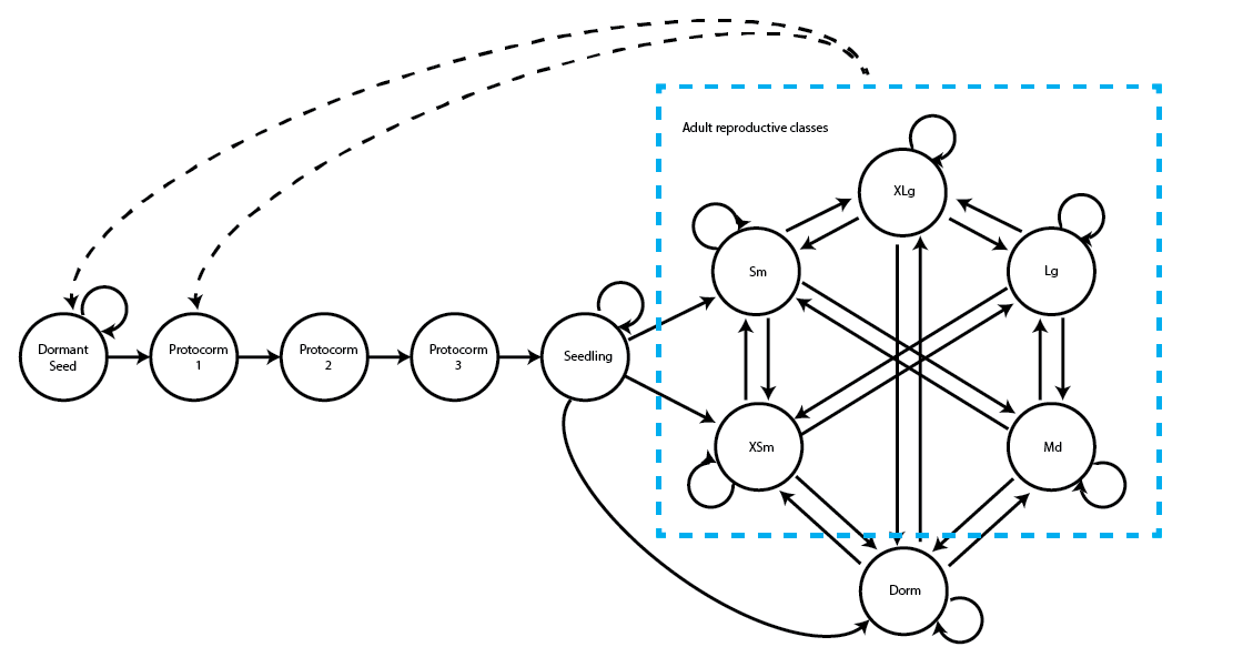
We have four raw MPMs. The first two, cypmatrix2r and cypmatrix2rp, are ahistorical MPMs at the population and patch level, respectively. The next two, cypmatrix3r and cypmatrix3rp, are historical MPMs at the population and patch level, respectively. Let’s see their summaries to jumpstart our memories about them.
summary(cypmatrix2r)
>
> This ahistorical lefkoMat object contains 5 matrices.
>
> Each matrix is square with 11 rows and columns, and a total of 121 elements.
> A total of 120 survival transitions were estimated, with 24 per matrix.
> A total of 40 fecundity transitions were estimated, with 8 per matrix.
> This lefkoMat object covers 1 population, 1 patch, and 5 time steps.
>
> The dataset contains a total of 74 unique individuals and 320 unique transitions.
>
> Survival probability sum check (each matrix represented by column in order):
>          [,1]  [,2]  [,3]  [,4]  [,5]
> Min.    0.000 0.050 0.050 0.000 0.050
> 1st Qu. 0.100 0.140 0.140 0.100 0.140
> Median  0.689 0.870 0.864 0.610 0.882
> Mean    0.552 0.629 0.629 0.528 0.627
> 3rd Qu. 1.000 1.000 1.000 0.960 1.000
> Max.    1.000 1.000 1.000 1.000 1.000
>
>
> Stages without connections leading to the rest of the life cycle found in matrices: 1 4
summary(cypmatrix2rp)
>
> This ahistorical lefkoMat object contains 15 matrices.
>
> Each matrix is square with 11 rows and columns, and a total of 121 elements.
> A total of 266 survival transitions were estimated, with 17.733 per matrix.
> A total of 70 fecundity transitions were estimated, with 4.667 per matrix.
> This lefkoMat object covers 1 population, 3 patches, and 5 time steps.
>
> The dataset contains a total of 74 unique individuals and 320 unique transitions.
>
> Survival probability sum check (each matrix represented by column in order):
>          [,1]  [,2]  [,3]  [,4]  [,5]  [,6]  [,7]  [,8]  [,9] [,10] [,11] [,12]
> Min.    0.000 0.000 0.000 0.000 0.000 0.000 0.050 0.050 0.000 0.050 0.000 0.000
> 1st Qu. 0.075 0.025 0.075 0.025 0.075 0.075 0.140 0.140 0.100 0.140 0.100 0.100
> Median  0.180 0.100 0.180 0.100 0.180 0.180 0.909 0.778 0.686 0.857 0.750 0.575
> Mean    0.457 0.361 0.471 0.328 0.417 0.464 0.631 0.611 0.530 0.631 0.562 0.523
> 3rd Qu. 0.955 0.769 1.000 0.592 0.781 1.000 1.000 1.000 0.955 1.000 1.000 1.000
> Max.    1.000 1.000 1.000 1.000 1.000 1.000 1.000 1.000 1.000 1.000 1.000 1.000
>         [,13] [,14] [,15]
> Min.    0.000 0.000 0.000
> 1st Qu. 0.075 0.075 0.100
> Median  0.180 0.180 0.750
> Mean    0.432 0.450 0.562
> 3rd Qu. 0.875 1.000 1.000
> Max.    1.000 1.000 1.000
>
>
> Stages without connections leading to the rest of the life cycle found in matrices: 1 2 3 4 5 6 9 11 12 13 14 15
summary(cypmatrix3r)
>
> This historical lefkoMat object contains 4 matrices.
>
> Each matrix is square with 121 rows and columns, and a total of 14641 elements.
> A total of 242 survival transitions were estimated, with 60.5 per matrix.
> A total of 54 fecundity transitions were estimated, with 13.5 per matrix.
> This lefkoMat object covers 1 population, 1 patch, and 4 time steps.
>
> The dataset contains a total of 74 unique individuals and 320 unique transitions.
>
> Survival probability sum check (each matrix represented by column in order):
>          [,1]  [,2]  [,3]  [,4]
> Min.    0.000 0.000 0.000 0.000
> 1st Qu. 0.000 0.000 0.000 0.000
> Median  0.000 0.000 0.000 0.000
> Mean    0.173 0.179 0.166 0.198
> 3rd Qu. 0.100 0.100 0.100 0.100
> Max.    1.000 1.000 1.000 1.000
>
>
> Stage-pairs without connections leading to them found in matrices: 1 2 3 4
summary(cypmatrix3rp)
>
> This historical lefkoMat object contains 12 matrices.
>
> Each matrix is square with 121 rows and columns, and a total of 14641 elements.
> A total of 516 survival transitions were estimated, with 43 per matrix.
> A total of 70 fecundity transitions were estimated, with 5.833 per matrix.
> This lefkoMat object covers 1 population, 3 patches, and 4 time steps.
>
> The dataset contains a total of 74 unique individuals and 320 unique transitions.
>
> Survival probability sum check (each matrix represented by column in order):
>          [,1]   [,2]   [,3]  [,4]  [,5]  [,6] [,7]  [,8]  [,9]  [,10] [,11]
> Min.    0.000 0.0000 0.0000 0.000 0.000 0.000 0.00 0.000 0.000 0.0000 0.000
> 1st Qu. 0.000 0.0000 0.0000 0.000 0.000 0.000 0.00 0.000 0.000 0.0000 0.000
> Median  0.000 0.0000 0.0000 0.000 0.000 0.000 0.00 0.000 0.000 0.0000 0.000
> Mean    0.107 0.0945 0.0851 0.101 0.158 0.158 0.14 0.169 0.119 0.0851 0.119
> 3rd Qu. 0.000 0.0000 0.0000 0.000 0.100 0.100 0.05 0.100 0.000 0.0000 0.000
> Max.    1.000 1.0000 1.0000 1.000 1.000 1.000 1.00 1.000 1.000 1.0000 1.000
>         [,12]
> Min.    0.000
> 1st Qu. 0.000
> Median  0.000
> Mean    0.144
> 3rd Qu. 0.000
> Max.    1.000
>
>
> Stage-pairs without connections leading to them found in matrices: 1 2 3 4 5 6 7 8 9 10 11 12
Next, let’s look again at the life history model for the function-based approach (figure 8.2; note that this is the same as figure 2.3).
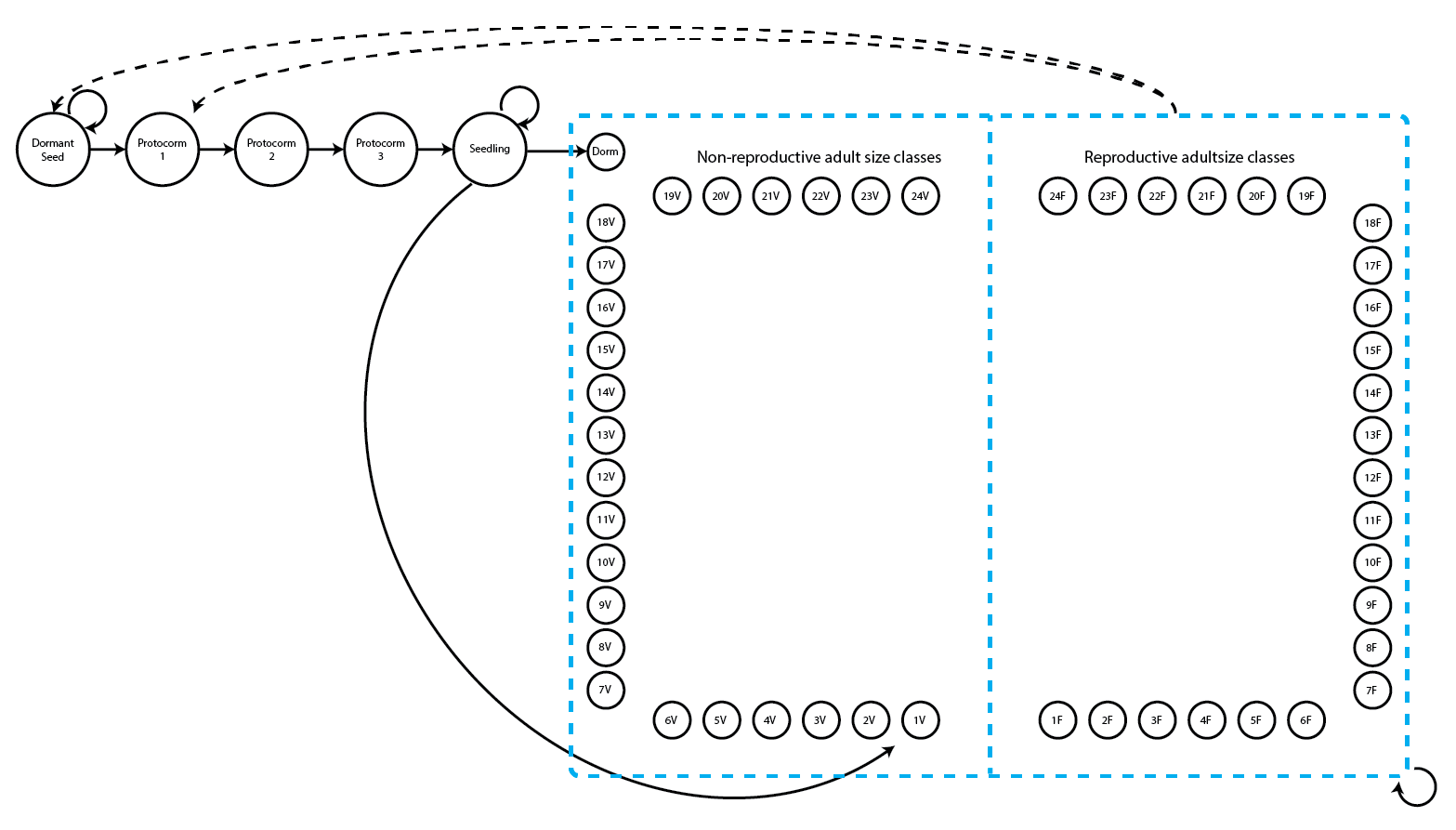
For this approach, we do not need actual MPMs, but we do need vital rate models. So, let’s see the model summaries in the lefkoMod object we will use.
summary(cypmodels2_env1)
> This LefkoMod object includes 5 linear models.
> Best-fit model criterion used: aicc&k
>
>
>
> Survival model:
> Generalized linear mixed model fit by maximum likelihood (Laplace
>   Approximation) [glmerMod]
>  Family: binomial  ( logit )
> Formula: alive3 ~ indcova2 + (1 | year2) + (1 | individ)
>    Data: surv.data
>       AIC       BIC    logLik -2*log(L)  df.resid
>  102.9757  118.0490  -47.4878   94.9757       316
> Random effects:
>  Groups  Name        Std.Dev.
>  individ (Intercept) 1197.97
>  year2   (Intercept)   89.74
> Number of obs: 320, groups:  individ, 74; year2, 5
> Fixed Effects:
> (Intercept)     indcova2
>      271.32        -2.19
> optimizer (Nelder_Mead) convergence code: 0 (OK) ; 0 optimizer warnings; 2 lme4 warnings
>
>
>
> Observation model:
> Generalized linear mixed model fit by maximum likelihood (Laplace
>   Approximation) [glmerMod]
>  Family: binomial  ( logit )
> Formula: obsstatus3 ~ size2added + (1 | year2) + (1 | individ)
>    Data: obs.data
>       AIC       BIC    logLik -2*log(L)  df.resid
>  118.2567  133.1117  -55.1284  110.2567       299
> Random effects:
>  Groups  Name        Std.Dev.
>  individ (Intercept) 1.078e-05
>  year2   (Intercept) 8.776e-01
> Number of obs: 303, groups:  individ, 70; year2, 5
> Fixed Effects:
> (Intercept)   size2added
>      2.4904       0.3134
> optimizer (Nelder_Mead) convergence code: 0 (OK) ; 0 optimizer warnings; 1 lme4 warnings
>
>
>
> Size model:
> Formula:          size3added ~ (1 | year2) + (1 | individ)
> Data: size.data
>       AIC       BIC    logLik -2*log(L)  df.resid
> 1008.2764 1022.9282 -500.1382 1000.2764       284
> Random-effects (co)variances:
>
> Conditional model:
>  Groups  Name        Std.Dev.
>  year2   (Intercept) 0.1109
>  individ (Intercept) 1.0561
>
> Number of obs: 288 / Conditional model: year2, 5; individ, 70
>
> Dispersion parameter for truncated_nbinom2 family (): 1.99e+07
>
> Fixed Effects:
>
> Conditional model:
> (Intercept)
>      0.5761
>
>
>
> Secondary size model:
> [1] 1
>
>
>
> Tertiary size model:
> [1] 1
>
>
>
> Reproductive status model:
> Generalized linear mixed model fit by maximum likelihood (Laplace
>   Approximation) [glmerMod]
>  Family: binomial  ( logit )
> Formula: repstatus3 ~ indcova2 + repstatus2 + size2added + (1 | year2) +
>     (1 | individ)
>    Data: repst.data
>       AIC       BIC    logLik -2*log(L)  df.resid
>  330.0418  352.0196 -159.0209  318.0418       282
> Random effects:
>  Groups  Name        Std.Dev.
>  individ (Intercept) 0.0002695
>  year2   (Intercept) 0.2479120
> Number of obs: 288, groups:  individ, 70; year2, 5
> Fixed Effects:
> (Intercept)     indcova2   repstatus2   size2added
>    -4.23766      0.02954      1.71091      0.17187
>
>
>
> Fecundity model:
> Formula:          feca2 ~ indcova2 + size2added + (1 | year2) + (1 | individ)
> Zero inflation:         ~size2added + (1 | year2) + (1 | individ)
> Data: fec.data
>       AIC       BIC    logLik -2*log(L)  df.resid
>  245.4867  270.4229 -113.7434  227.4867       109
> Random-effects (co)variances:
>
> Conditional model:
>  Groups  Name        Std.Dev.
>  year2   (Intercept) 0.2517
>  individ (Intercept) 0.1927
>
> Zero-inflation model:
>  Groups  Name        Std.Dev.
>  year2   (Intercept) 2.072e-04
>  individ (Intercept) 3.951e-08
>
> Number of obs: 118 / Conditional model: year2, 5; individ, 51 / Zero-inflation model: year2, 5; individ, 51
>
> Fixed Effects:
>
> Conditional model:
> (Intercept)     indcova2   size2added
>     1.68997     -0.02397      0.06174
>
> Zero-inflation model:
> (Intercept)   size2added
>       3.927       -1.618
>
>
> Juvenile survival model:
> [1] 1
>
>
>
> Juvenile observation model:
> [1] 1
>
>
>
> Juvenile size model:
> [1] 1
>
>
>
> Juvenile secondary size model:
> [1] 1
>
>
>
> Juvenile tertiary size model:
> [1] 1
>
>
>
> Juvenile reproduction model:
> [1] 1
>
>
>
> Juvenile maturity model:
> [1] 1
>
>
>
>
>
> Number of models in survival table: 7
>
> Number of models in observation table: 8
>
> Number of models in size table: 8
>
> Number of models in secondary size table: 1
>
> Number of models in tertiary size table: 1
>
> Number of models in reproduction status table: 8
>
> Number of models in fecundity table: 64
>
> Number of models in juvenile survival table: 1
>
> Number of models in juvenile observation table: 1
>
> Number of models in juvenile size table: 1
>
> Number of models in juvenile secondary size table: 1
>
> Number of models in juvenile tertiary size table: 1
>
> Number of models in juvenile reproduction table: 1
>
> Number of models in juvenile maturity table: 1
>
>
>
>
>
> General model parameter names (column 1), and
> specific names used in these models (column 2):
>                       parameter_names mainparams
> 1                              time t      year2
> 2                          individual    individ
> 3                               patch      patch
> 4                   alive in time t+1      surv3
> 5                observed in time t+1       obs3
> 6                   sizea in time t+1      size3
> 7                   sizeb in time t+1     sizeb3
> 8                   sizec in time t+1     sizec3
> 9     reproductive status in time t+1     repst3
> 10              fecundity in time t+1       fec3
> 11                fecundity in time t       fec2
> 12                    sizea in time t      size2
> 13                  sizea in time t-1      size1
> 14                    sizeb in time t     sizeb2
> 15                  sizeb in time t-1     sizeb1
> 16                    sizec in time t     sizec2
> 17                  sizec in time t-1     sizec1
> 18      reproductive status in time t     repst2
> 19    reproductive status in time t-1     repst1
> 20        maturity status in time t+1     matst3
> 21          maturity status in time t     matst2
> 22                      age in time t        age
> 23                  density in time t    density
> 24   individual covariate a in time t   indcova2
> 25 individual covariate a in time t-1   indcova1
> 26   individual covariate b in time t   indcovb2
> 27 individual covariate b in time t-1   indcovb1
> 28   individual covariate c in time t   indcovc2
> 29 individual covariate c in time t-1   indcovc1
> 30              stage group in time t     group2
> 31            stage group in time t-1     group1
> 32       annual covariate a in time t  annucova2
> 33     annual covariate a in time t-1  annucova1
> 34       annual covariate b in time t  annucovb2
> 35     annual covariate b in time t-1  annucovb1
> 36       annual covariate c in time t  annucovc2
> 37     annual covariate c in time t-1  annucovc1
>
>
>
>
>
> Quality control:
>
> Survival model estimated with 74 individuals and 320 individual transitions.
> Survival model accuracy is 1.
> Observation status model estimated with 70 individuals and 303 individual transitions.
> Observation status model accuracy is 0.95.
> Primary size model estimated with 70 individuals and 288 individual transitions.
> Primary size model R-squared is 0.822.
> Secondary size model not estimated.
> Tertiary size model not estimated.
> Reproductive status model estimated with 70 individuals and 288 individual transitions.
> Reproductive status model accuracy is 0.719.
> Fecundity model estimated with 51 individuals and 118 individual transitions.
> Fecundity model R-squared is 0.524.
> Juvenile survival model not estimated.
> Juvenile observation status model not estimated.
> Juvenile primary size model not estimated.
> Juvenile secondary size model not estimated.
> Juvenile tertiary size model not estimated.
> Juvenile reproductive status model not estimated.
> Juvenile maturity status model not estimated.
We will use these two approaches to conduct three major types of density dependent analyses:
- Density dependent deterministic projections
- Ordered or cyclical density dependent simulations
- Replicated density dependent simulations assuming temporal stochasticity
Projection styles 1 and 2 assume no randomness and so we assume that users are not interested in producing replicates for those styles. However, both projection3() and f_projection3() allow replication for all styles. Let’s begin with the first style of projection.
11.2.1 Density dependent deterministic projections involving pre-existing MPMs
In the simplest density dependent analysis, a single matrix is projected forward with some elements altered at each time step according to some function of population size, \(N\). We might conduct such an analysis if we believe that density has some role in population dynamics, but we are not concerned with any other variation or influences. For example, we might suspect that natural selection is at work in our study population, and natural selection often works under the assumption of conspecific competition. Alternatively, we might believe that the stability of the population dynamics that we see might be due to a limit on the number of individuals that a community can support. In other cases, we may see actual population trends that suggest a role for density, such as cycles of different periods.
Let’s start our analysis by projecting the mean ahistorical matrix in our raw MPM forward using four different parameterizations of the Ricker function modifying germination. Our first step will be to create four density frames (lefkoDens objects), which will describe the relationships between the matrices and density.
c2d_1 <- density_input(cypmean2, stage3 = c("P1", "P1"), stage2= c("SD", "rep"),
  style = 1, time_delay = 1, alpha = 0.05, beta = 0, type = c(2, 2))
c2d_2 <- density_input(cypmean2, stage3 = c("P1", "P1"), stage2= c("SD", "rep"),
  style = 1, time_delay = 1, alpha = 1, beta = 0, type = c(2, 2))
c2d_3 <- density_input(cypmean2, stage3 = c("P1", "P1"), stage2= c("SD", "rep"),
  style = 1, time_delay = 1, alpha = 0.05, beta = 0.0005, type = c(2, 2))
c2d_4 <- density_input(cypmean2, stage3 = c("P1", "P1"), stage2= c("SD", "rep"),
  style = 1, time_delay = 1, alpha = 1, beta = 0.0005, type = c(2, 2))

c2d_1
>   stage3 stage2 stage1 age2 style alpha beta time_delay type type_t12
> 1     P1     SD     NA   NA     1  0.05    0          1    2        1
> 2     P1    XSm     NA   NA     1  0.05    0          1    2        1
> 3     P1     Sm     NA   NA     1  0.05    0          1    2        1
> 4     P1     Md     NA   NA     1  0.05    0          1    2        1
> 5     P1     Lg     NA   NA     1  0.05    0          1    2        1
> 6     P1    XLg     NA   NA     1  0.05    0          1    2        1

c2d_2
>   stage3 stage2 stage1 age2 style alpha beta time_delay type type_t12
> 1     P1     SD     NA   NA     1     1    0          1    2        1
> 2     P1    XSm     NA   NA     1     1    0          1    2        1
> 3     P1     Sm     NA   NA     1     1    0          1    2        1
> 4     P1     Md     NA   NA     1     1    0          1    2        1
> 5     P1     Lg     NA   NA     1     1    0          1    2        1
> 6     P1    XLg     NA   NA     1     1    0          1    2        1

c2d_3
>   stage3 stage2 stage1 age2 style alpha  beta time_delay type type_t12
> 1     P1     SD     NA   NA     1  0.05 5e-04          1    2        1
> 2     P1    XSm     NA   NA     1  0.05 5e-04          1    2        1
> 3     P1     Sm     NA   NA     1  0.05 5e-04          1    2        1
> 4     P1     Md     NA   NA     1  0.05 5e-04          1    2        1
> 5     P1     Lg     NA   NA     1  0.05 5e-04          1    2        1
> 6     P1    XLg     NA   NA     1  0.05 5e-04          1    2        1

c2d_4
>   stage3 stage2 stage1 age2 style alpha  beta time_delay type type_t12
> 1     P1     SD     NA   NA     1     1 5e-04          1    2        1
> 2     P1    XSm     NA   NA     1     1 5e-04          1    2        1
> 3     P1     Sm     NA   NA     1     1 5e-04          1    2        1
> 4     P1     Md     NA   NA     1     1 5e-04          1    2        1
> 5     P1     Lg     NA   NA     1     1 5e-04          1    2        1
> 6     P1    XLg     NA   NA     1     1 5e-04          1    2        1
Determining the values of \(\alpha\) and \(\beta\) to use for the alpha and beta options generally takes a great deal of extra work. We have done this work separately and present only four interesting combinations that produce contrasting results in this case. Note also that the style, alpha, and beta terms can be vectors if necessary, giving different kinds of density dependence and different values for \(\alpha\) and \(\beta\) when needed.
Now let’s conduct some short simulations. We will only project forward 100 time steps, and we will enforce hard substochasticity.
cypproj2_d1 <- projection3(cypmean2, times = 100, substoch = 2, density = c2d_1)
> Warning: This lefkoMat object appears to be a set of mean matrices. Will
> project only the mean.
cypproj2_d2 <- projection3(cypmean2, times = 100, substoch = 2, density = c2d_2)
> Warning: This lefkoMat object appears to be a set of mean matrices. Will
> project only the mean.
cypproj2_d3 <- projection3(cypmean2, times = 100, substoch = 2, density = c2d_3)
> Warning: This lefkoMat object appears to be a set of mean matrices. Will
> project only the mean.
cypproj2_d4 <- projection3(cypmean2, times = 100, substoch = 2, density = c2d_4)
> Warning: This lefkoMat object appears to be a set of mean matrices. Will
> project only the mean.

summary(cypproj2_d1)
>
> The input lefkoProj object covers 1 population-patches.
> It is a single projection including 100 projected steps per replicate, and 1 replicates, respectively.
> The number of replicates with population size above the threshold size of 1 is as in
> the following matrix, with pop-patches given by column and milepost times given by row:
> $milepost_sums
>      1 1
> 0      1
> 0.25   1
> 0.5    1
> 0.75   1
> 1      1
>
> $extinction_times
> [1] NA

summary(cypproj2_d2)
>
> The input lefkoProj object covers 1 population-patches.
> It is a single projection including 100 projected steps per replicate, and 1 replicates, respectively.
> The number of replicates with population size above the threshold size of 1 is as in
> the following matrix, with pop-patches given by column and milepost times given by row:
> $milepost_sums
>      1 1
> 0      1
> 0.25   1
> 0.5    1
> 0.75   1
> 1      1
>
> $extinction_times
> [1] NA

summary(cypproj2_d3)
>
> The input lefkoProj object covers 1 population-patches.
> It is a single projection including 100 projected steps per replicate, and 1 replicates, respectively.
> The number of replicates with population size above the threshold size of 1 is as in
> the following matrix, with pop-patches given by column and milepost times given by row:
> $milepost_sums
>      1 1
> 0      1
> 0.25   1
> 0.5    1
> 0.75   1
> 1      1
>
> $extinction_times
> [1] NA

summary(cypproj2_d4)
>
> The input lefkoProj object covers 1 population-patches.
> It is a single projection including 100 projected steps per replicate, and 1 replicates, respectively.
> The number of replicates with population size above the threshold size of 1 is as in
> the following matrix, with pop-patches given by column and milepost times given by row:
> $milepost_sums
>      1 1
> 0      1
> 0.25   1
> 0.5    1
> 0.75   1
> 1      1
>
> $extinction_times
> [1] NA
Let’s plot these projections together and take a look (figure 11.1).
par(mfrow = c(2, 2))

plot(cypproj2_d1)
title("a)", adj = 0)

plot(cypproj2_d2, ylab = "")
title("b)", adj = 0)

plot(cypproj2_d3)
title("c)", adj = 0)

plot(cypproj2_d4, ylab = "")
title("d)", adj = 0)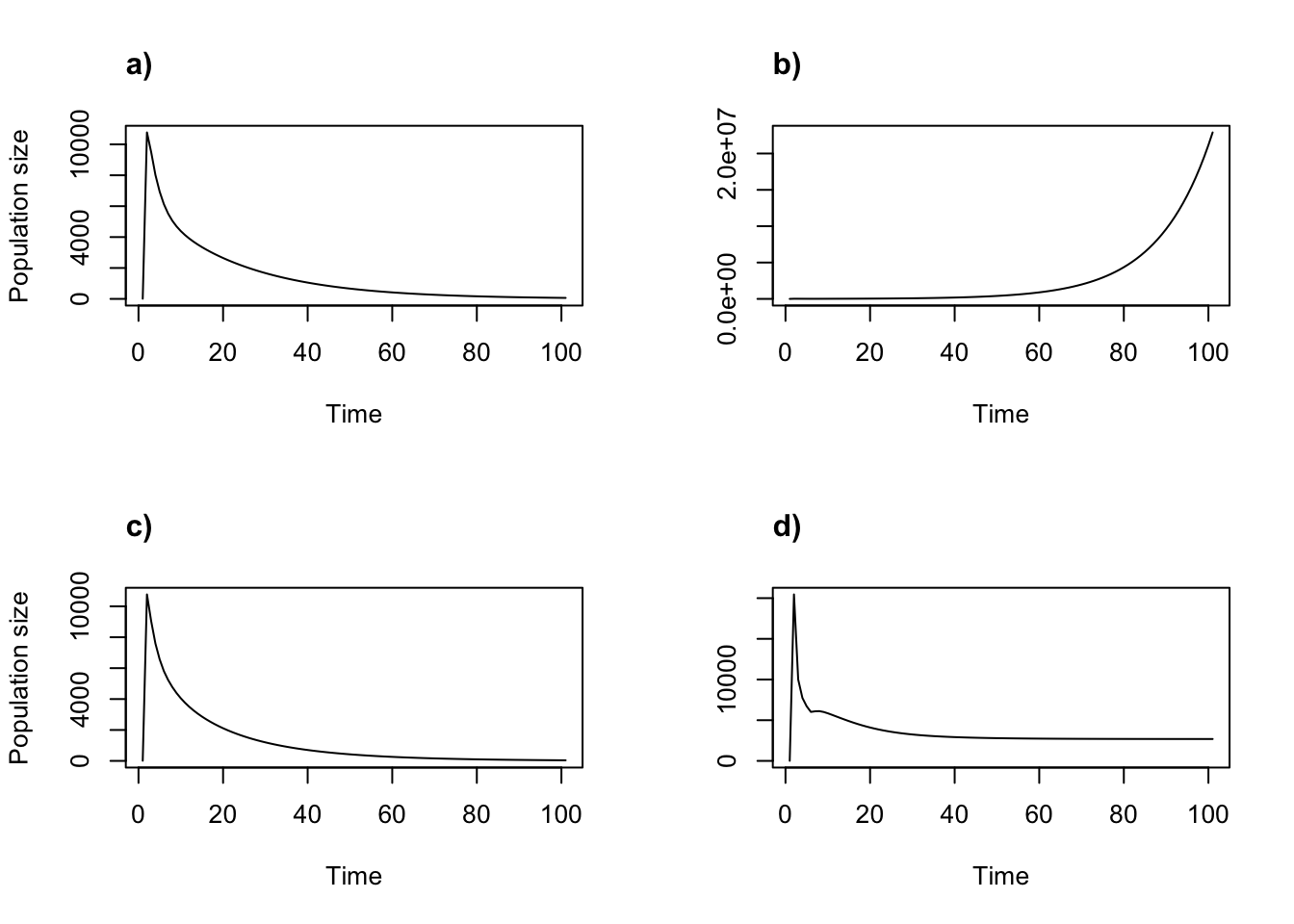
Figure 11.1: Density dependent projections using the two-parameter Ricker function. (a) alpha = 0.05, beta = 0; (b) alpha = 1, beta = 0; (c) alpha = 0.05, beta = 0.0005; and (d) alpha = 1, beta = 0.0005.
Each projection behaves a little differently. Notably, raising \(\alpha\) from 0.05 to 1 appears to keep the population from declining to extinction (b, d). Changing \(\beta\) from 0 to 0.0005 leads to a seemingly stabilized population size (d) rather than permitting exponential growth (b). The patterns are contingent on this particular MPM and to some extent on the start vector, meaning that other MPMs will yield different patterns with these \(\alpha\) and \(\beta\) values.
The above projections assumed that fractional individuals could live and reproduce. Let’s prevent that behavior by setting integeronly = TRUE, as below.
cypproj2_d1_int <- projection3(cypmean2, times = 100, substoch = 2,
  integeronly = TRUE, density = c2d_1)
> Warning: This lefkoMat object appears to be a set of mean matrices. Will
> project only the mean.
cypproj2_d2_int <- projection3(cypmean2, times = 100, substoch = 2,
  integeronly = TRUE, density = c2d_2)
> Warning: This lefkoMat object appears to be a set of mean matrices. Will
> project only the mean.
cypproj2_d3_int <- projection3(cypmean2, times = 100, substoch = 2,
  integeronly = TRUE, density = c2d_3)
> Warning: This lefkoMat object appears to be a set of mean matrices. Will
> project only the mean.
cypproj2_d4_int <- projection3(cypmean2, times = 100, substoch = 2,
  integeronly = TRUE, density = c2d_4)
> Warning: This lefkoMat object appears to be a set of mean matrices. Will
> project only the mean.

par(mfrow = c(2, 2))

plot(cypproj2_d1_int)
title("a)", adj = 0)

plot(cypproj2_d2_int, ylab = "")
title("b)", adj = 0)

plot(cypproj2_d3_int)
title("c)", adj = 0)

plot(cypproj2_d4_int, ylab = "")
title("d)", adj = 0)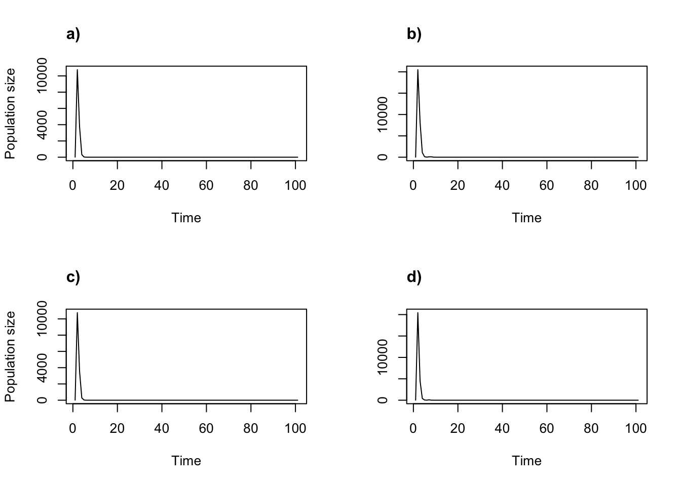
Figure 11.2: Density dependent projections using the two-parameter Ricker function and fractional individuals not allowed. (a) alpha = 0.05, beta = 0; (b) alpha = 1, beta = 0; (c) alpha = 0.05, beta = 0.0005; and (d) alpha = 1, beta = 0.0005.
Both the graphs and the associated summaries (not shown) suggest extinction in all cases, and very quickly. We urge users to think carefully through their assumptions prior to analysis.
Let’s also try four parameterizations of the two-parameter Beverton-Holt function.
c2d_5 <- density_input(cypmean2, stage3 = c("P1", "P1"), stage2= c("SD", "rep"),
  style = 2, time_delay = 1, alpha = 0.05, beta = 0, type = c(2, 2))
c2d_6 <- density_input(cypmean2, stage3 = c("P1", "P1"), stage2= c("SD", "rep"),
  style = 2, time_delay = 1, alpha = 1, beta = 0, type = c(2, 2))
c2d_7 <- density_input(cypmean2, stage3 = c("P1", "P1"), stage2= c("SD", "rep"),
  style = 2, time_delay = 1, alpha = 0.05, beta = 1, type = c(2, 2))
c2d_8 <- density_input(cypmean2, stage3 = c("P1", "P1"), stage2= c("SD", "rep"),
  style = 2, time_delay = 1, alpha = 1, beta = 1, type = c(2, 2))

cypproj2_d5 <- projection3(cypmean2, times = 100, substoch = 2, density = c2d_5)
> Warning: This lefkoMat object appears to be a set of mean matrices. Will
> project only the mean.
cypproj2_d6 <- projection3(cypmean2, times = 100, substoch = 2, density = c2d_6)
> Warning: This lefkoMat object appears to be a set of mean matrices. Will
> project only the mean.
cypproj2_d7 <- projection3(cypmean2, times = 100, substoch = 2, density = c2d_7)
> Warning: This lefkoMat object appears to be a set of mean matrices. Will
> project only the mean.
cypproj2_d8 <- projection3(cypmean2, times = 100, substoch = 2, density = c2d_8)
> Warning: This lefkoMat object appears to be a set of mean matrices. Will
> project only the mean.
Now let’s plot them (figure 11.3).
par(mfrow = c(2, 2))

plot(cypproj2_d5)
title("a)", adj = 0)

plot(cypproj2_d6, ylab = "")
title("b)", adj = 0)

plot(cypproj2_d7)
title("c)", adj = 0)

plot(cypproj2_d8, ylab = "")
title("d)", adj = 0)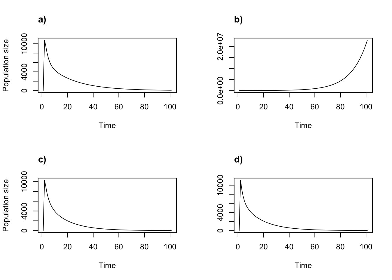
Figure 11.3: Density dependent projections using the two-parameter Beverton-Holt function. (a) alpha = 0.05, beta = 0; (b) alpha = 1, beta = 0; (c) alpha = 0.05, beta = 1; and (d) alpha = 1, beta = 1.
The Beverton-Holt function is less likely to produce unusual shapes to population projections than the Ricker function. For example, it is generally not capable of producing chaos. This is both a strength and a weakness - its simplicity makes it attractive in many situations, but prevents it from matching reality in others. Users will need to explore the different density functions under different parameterizations to decide on an appropriate parameterization of density dependence for their research.
11.2.2 Density dependent, function-based deterministic projections
Next let’s try density dependent deterministic projection with the function-based approach. This style of projection is particularly useful when we need to set some specific parameters prior to the run, such as specific values for individual covariates. Here, we cannot use a mean matrix apprach, and so we have two possible choices - we may either choose a single year to run (our vital rates all include random year terms) with our projected covariate value(s), or we may try a specific sequence of years. There are different merits to both approaches.
Density dependent projections can run in two ways using function f_projection3(). The first involves setting density dependence relationships in matrix elements, just as is done with function projection3(). Users may use the two-parameter Ricker function, two-parameter Beverton-Holt function, the Usher function, and the logistic function, and need to specify which transitions to apply these to. Likewise, function f_projection3() can also enforce substochasticity, with both a mild setting forcing survival-transition elements to be in the range [0, 1], and a hard setting forcing survival-transition column sums to this range. Let’s see a simple example. Remember that, as in start_input(), we need to provide density_input() with an example MPM with the same characteristics as the projection that we will run, so that the function can infer the proper stage distribution and produce the proper output vector.
cyp_ex <- flefko2(year = 2004, stageframe = cypframe_fb,
  supplement = cypsupp2_fb, modelsuite = cypmodels2_env1, data = cypfb_env)

c2d <- density_input(cyp_ex, stage3 = c("P1", "P1"),
  stage2 = c("SD", "rep"), style = 1, time_delay = 1, alpha = 1, beta = 0.0005,
  type = c(2, 2))

trial2f_13 <- f_projection3(data = cypfb_env, format = 3, stageframe = cypframe_fb,
  supplement = cypsupp2_fb, modelsuite = cypmodels2_env1, times = 101,
  year = 2007, ind_terms = mean_real, density = c2d)
> Warning: Option patch not set, so will set to first patch/population.
> Warning: Too few values of individual covariates have been supplied. Some will
> be cycled.

summary(trial2f_13)
>
> The input lefkoProj object covers 1 population-patches.
> It is a single projection including 101 projected steps per replicate, and 1 replicates, respectively.
> The number of replicates with population size above the threshold size of 1 is as in
> the following matrix, with pop-patches given by column and milepost times given by row:
> $milepost_sums
>      1 1
> 0      1
> 0.25   1
> 0.5    1
> 0.75   1
> 1      1
>
> $extinction_times
> [1] NA
We can compare the results to a density independent version assuming the year2 value for 2007 (figure 11.4). Note the extreme impact that density dependence has on the population trajectory.
ind_frame_2 <- cbind.data.frame(inda = pred_vals_2070to90, indb = 0, indc = 0)

trial2f_2 <- f_projection3(data = cypfb_env, format = 3, year = 2007,
  stageframe = cypframe_fb, supplement = cypsupp2_fb, times = 21,
  modelsuite = cypmodels2_env1, ind_terms = ind_frame_2)
> Warning: Option patch not set, so will set to first patch/population.

par(mfrow=c(1,2))

plot(trial2f_2)
title("a)", adj = 0)

plot(trial2f_13, ylab = "")
title("b)", adj = 0)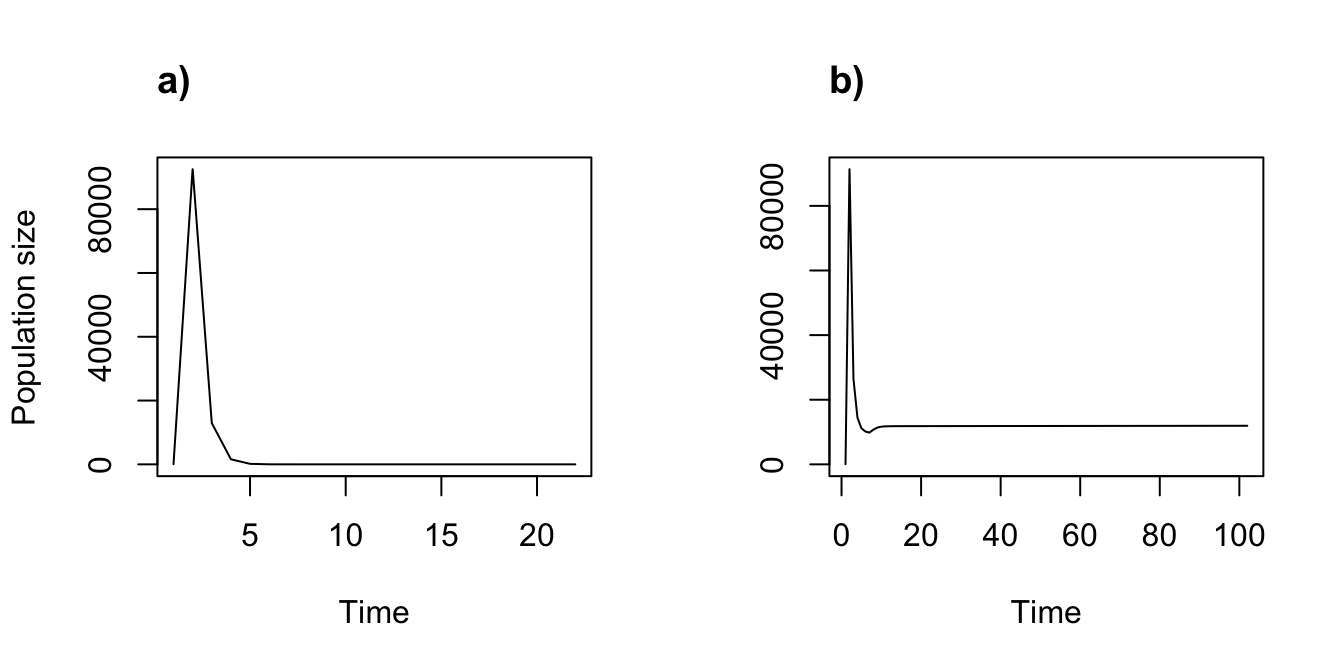
Figure 11.4: Density independent (a) vs. density dependent (b) function-based projections
Function f_projection3() can also run density dependent simulations assuming that vital rates are density dependent. This situation allows us to modify the vital rates used to estimate the matrix elements. As before, it is possible to use the two-parameter Ricker function, the two-parameter Beverton-Holt function, the Usher function, or the logistic function. Let’s try a simulation in which we make survival and fecundity density dependent, using the Ricker function for both. We will use the density_vr() function for this purpose.
vr1 <- density_vr(density_yn = c(T, F, F, F, F, F, T, F, F, F, F, F, F, F),
  style = c(1, 0, 0, 0, 0, 0, 1, 0, 0, 0, 0, 0, 0, 0),
  alpha = c(1, 0, 0, 0, 0, 0, 1, 0, 0, 0, 0, 0, 0, 0),
  beta = c(-0.0000000005, 0, 0, 0, 0, 0, 0.0000000003, 0, 0, 0, 0, 0, 0, 0))

trial2f_14 <- f_projection3(data = cypfb_env, format = 3, stageframe = cypframe_fb,
  supplement = cypsupp2_fb, modelsuite = cypmodels2_env1, times = 101,
  year = 2007, ind_terms = mean_real, density_vr = vr1, substoch = 2)
> Warning: Option patch not set, so will set to first patch/population.
> Warning: Too few values of individual covariates have been supplied. Some will
> be cycled.

summary(trial2f_14)
>
> The input lefkoProj object covers 1 population-patches.
> It is a single projection including 101 projected steps per replicate, and 1 replicates, respectively.
> The number of replicates with population size above the threshold size of 1 is as in
> the following matrix, with pop-patches given by column and milepost times given by row:
> $milepost_sums
>      1 1
> 0      1
> 0.25   1
> 0.5    1
> 0.75   1
> 1      1
>
> $extinction_times
> [1] NA
In our density_vr() call, we need to set the density dependence relationships for 14 different vital rates that are used by the function-based matrix estimators in lefko3. The 14 models, in order, are: survival, observation, primary size, secondary size, tertiary size, reproduction status, and fecundity, followed by juvenile survival, juvenile observation, juvenile primary size, juvenile secondary size, juvenile tertiary size, juvenile reproduction status, and juvenile maturity status. The density_yn option stipulates with TRUE and FALSE statements which of these will be modified, and the style, alpha, beta, and time_delay arguments give the settings to use (last option not shown). Let’s plot the results (figure 11.5).
par(mfrow=c(1,2))

plot(trial2f_2)
title("a)", adj = 0)

plot(trial2f_14, ylab = "")
title("b)", adj = 0)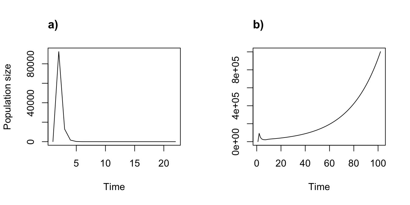
Figure 11.5: Density independent (a) vs. density dependent (b) function-based projections with density dependent vital rates
We see a dramatic difference in projected population dynamics, resulting from two density dependent vital rates. Note also the contrast with our previous case of density dependence, which caused a population drop after an initial spike. Here, in contrast, the population is growing explosively.
11.2.3 Ordered or cyclical density dependent simulations using pre-existing MPMs
We have already seen that we can set our projections to run through a specific sequence of years. This sequence can be combined with density dependence in any way that we wish. Here, we conduct a density dependent projection using the raw Cypripedium MPM. We will set the first ten time steps to switch repeatedly between two wet years (2007 and 2008), followed by ten time steps of switching between two drier years (2004 and 2005). To make things interesting in our 20 year projection, we will utilize an Usher function with \(\alpha = 1\) and \(\beta = 0\), and our start frame with 1000 3rd year protocorms and 100 dormant adults.
year_order <- c(2007, 2008, 2007, 2008, 2007, 2008, 2007, 2008, 2007, 2008,
  2004, 2005, 2004, 2005, 2004, 2005, 2004, 2005, 2004, 2005)

c2d_9 <- density_input(cypmean2, stage3 = c("P1", "P1"), stage2= c("SD", "rep"),
  style = 3, time_delay = 1, alpha = 1, beta = 0, type = c(2, 2))

c2m_sv <- start_input(cypmean2, stage2 = c("P3", "Dorm"), value = c(1000, 100))

cypproj2_ord1d <- projection3(cypmatrix2r, year = year_order, times = 20,
  start_frame = c2m_sv, density = c2d_9)

summary(cypproj2_ord1d)
>
> The input lefkoProj object covers 1 population-patches.
> It is a single projection including 20 projected steps per replicate, and 1 replicates, respectively.
> The number of replicates with population size above the threshold size of 1 is as in
> the following matrix, with pop-patches given by column and milepost times given by row:
> $milepost_sums
>      1 1
> 0      1
> 0.25   1
> 0.5    1
> 0.75   1
> 1      1
>
> $extinction_times
> [1] NA
As before, if the sequence of years noted in the year option is shorter than the time steps designated in the times option, then lefko3 will cycle through the sequences of years until the projection is done. For example, if we leave the times option out from the above projection, then lefko3 will assume the default of 10,000 time steps, and cycle through our 20 defined years over and over, as below.
cypproj2_ord2d <- projection3(cypmatrix2r, year = year_order,
  start_frame = c2m_sv, density = c2d_9)

summary(cypproj2_ord2d)
>
> The input lefkoProj object covers 1 population-patches.
> It is a single projection including 10000 projected steps per replicate, and 1 replicates, respectively.
> The number of replicates with population size above the threshold size of 1 is as in
> the following matrix, with pop-patches given by column and milepost times given by row:
> $milepost_sums
>      1 1
> 0      1
> 0.25   0
> 0.5    0
> 0.75   0
> 1      0
>
> $extinction_times
> [1] NA
Let’s see plots of these projections (figure 11.6).
par(mfrow=c(1,2))

plot(cypproj2_ord1d)
title("a)", adj = 0)

plot(cypproj2_ord2d, ylab = "")
title("b)", adj = 0)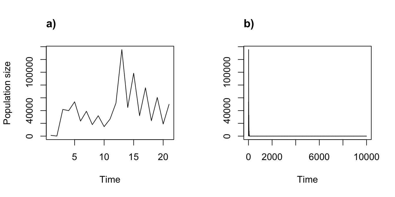
Figure 11.6: Ordered, density dependent projections can be cyclical. (a) A 20 year ordered projection. (b) A 10,000 year projection cycling through 20 ordered years
It appears that this particular form of density dependence leads to extinction fairly early on, though only after some strong fluctuations.
Projecting a full MPM with multiple annual matrices defaults to cycling through the matrices in order, even when density dependence is set. Let’s try the first four Ricker projections again, but this time using the full ahistorical MPM rather than the arithmetic mean matrix to allow cycling of year sequences.
cypproj2r_d1 <- projection3(cypmatrix2r, times = 100, substoch = 2,
  density = c2d_1)
cypproj2r_d2 <- projection3(cypmatrix2r, times = 100, substoch = 2,
  density = c2d_2)
cypproj2r_d3 <- projection3(cypmatrix2r, times = 100, substoch = 2,
  density = c2d_3)
cypproj2r_d4 <- projection3(cypmatrix2r, times = 100, substoch = 2,
  density = c2d_4)

summary(cypproj2r_d1)
>
> The input lefkoProj object covers 1 population-patches.
> It is a single projection including 100 projected steps per replicate, and 1 replicates, respectively.
> The number of replicates with population size above the threshold size of 1 is as in
> the following matrix, with pop-patches given by column and milepost times given by row:
> $milepost_sums
>      1 1
> 0      1
> 0.25   1
> 0.5    1
> 0.75   1
> 1      1
>
> $extinction_times
> [1] NA

summary(cypproj2r_d2)
>
> The input lefkoProj object covers 1 population-patches.
> It is a single projection including 100 projected steps per replicate, and 1 replicates, respectively.
> The number of replicates with population size above the threshold size of 1 is as in
> the following matrix, with pop-patches given by column and milepost times given by row:
> $milepost_sums
>      1 1
> 0      1
> 0.25   1
> 0.5    1
> 0.75   1
> 1      1
>
> $extinction_times
> [1] NA

summary(cypproj2r_d3)
>
> The input lefkoProj object covers 1 population-patches.
> It is a single projection including 100 projected steps per replicate, and 1 replicates, respectively.
> The number of replicates with population size above the threshold size of 1 is as in
> the following matrix, with pop-patches given by column and milepost times given by row:
> $milepost_sums
>      1 1
> 0      1
> 0.25   1
> 0.5    1
> 0.75   1
> 1      1
>
> $extinction_times
> [1] NA

summary(cypproj2r_d4)
>
> The input lefkoProj object covers 1 population-patches.
> It is a single projection including 100 projected steps per replicate, and 1 replicates, respectively.
> The number of replicates with population size above the threshold size of 1 is as in
> the following matrix, with pop-patches given by column and milepost times given by row:
> $milepost_sums
>      1 1
> 0      1
> 0.25   1
> 0.5    1
> 0.75   1
> 1      1
>
> $extinction_times
> [1] NA
Let’s see what these projections look like (11.7).
par(mfrow=c(2, 2))

plot(cypproj2r_d1)
title("a)", adj = 0)

plot(cypproj2r_d2, ylab = "")
title("b)", adj = 0)

plot(cypproj2r_d3)
title("c)", adj = 0)

plot(cypproj2r_d4, ylab = "")
title("d)", adj = 0)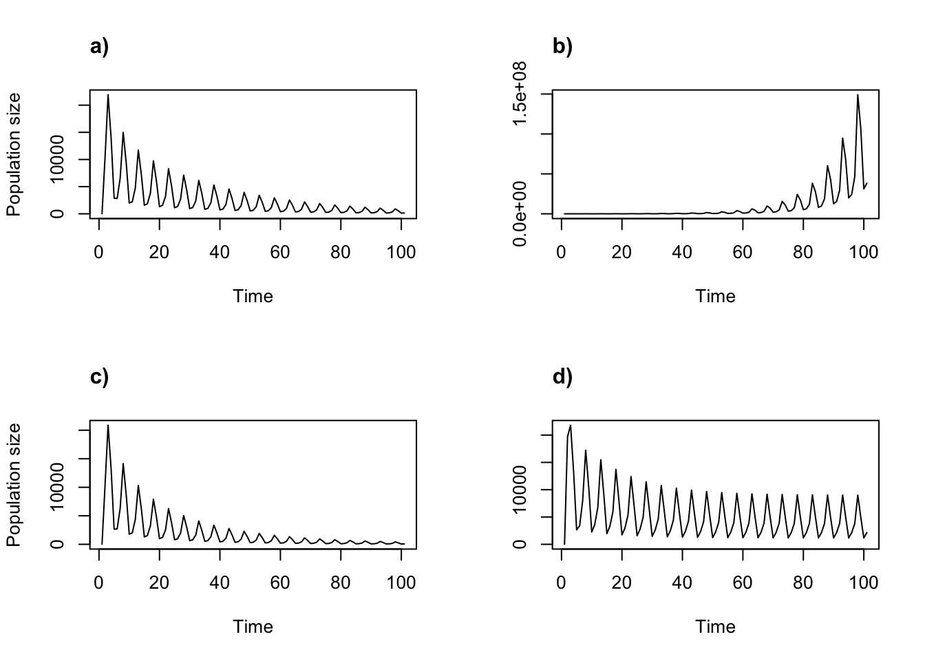
Figure 11.7: Cyclical density dependent projections using the Ricker function
We can see the obvious cycles in all projections. The population seems to be on the road to extinction in plots a) and c). Projection b) appears to show a growing population, while d) seems to be entering a stable oscillation.
11.2.4 Ordered / cyclical, density-dependent function-based projections of a specific time length
The vital rate models developed with modelsearch() generally include year2 terms denoting time t. These are terms within a categorical variable, and so each year has its own value. If we do not specify a specific year to project, then f_projection3() will cycle through the years in the dataset in order for the number of time steps set, using the appropriate year2 term in each vital rate model used to estimate each matrix at each time step. Alternatively, if the year option is set to a vector of years, then these particular years will cycle in order for the number of time steps set. Note, however, that this function only sets the values for the categorical year2 term in the vital rate models - any related terms, such as individual covariates, are unaffected by this.
We can also use f_projection() to run density dependent projections cycling through a specific set of year2 terms. Here is an example cycling through all terms in a density dependent, function-based projection. We will set the individual covariate to mean annual precipitation.
trial2f_15 <- f_projection3(data = cypfb_env, format = 3, stageframe = cypframe_fb,
  supplement = cypsupp2_fb, modelsuite = cypmodels2_env1, times = 101,
  ind_terms = mean_real, density = c2d)
> Warning: Option year not set, so will cycle through existing years.
> Warning: Option patch not set, so will set to first patch/population.
> Warning: Too few values of individual covariates have been supplied. Some will
> be cycled.

summary(trial2f_15)
>
> The input lefkoProj object covers 1 population-patches.
> It is a single projection including 101 projected steps per replicate, and 1 replicates, respectively.
> The number of replicates with population size above the threshold size of 1 is as in
> the following matrix, with pop-patches given by column and milepost times given by row:
> $milepost_sums
>      1 1
> 0      1
> 0.25   1
> 0.5    1
> 0.75   1
> 1      1
>
> $extinction_times
> [1] NA
Here is a further set cycling through just three particular years: 2005, 2006, and 2008.
trial2f_16 <- f_projection3(data = cypfb_env, format = 3, stageframe = cypframe_fb,
  supplement = cypsupp2_fb, modelsuite = cypmodels2_env1, times = 101,
  year = c(2005, 2006, 2008), ind_terms = mean_real, density = c2d)
> Warning: Option patch not set, so will set to first patch/population.
> Warning: Too few values of individual covariates have been supplied. Some will
> be cycled.

summary(trial2f_16)
>
> The input lefkoProj object covers 1 population-patches.
> It is a single projection including 101 projected steps per replicate, and 1 replicates, respectively.
> The number of replicates with population size above the threshold size of 1 is as in
> the following matrix, with pop-patches given by column and milepost times given by row:
> $milepost_sums
>      1 1
> 0      1
> 0.25   1
> 0.5    1
> 0.75   1
> 1      1
>
> $extinction_times
> [1] NA
As before, we can also run a specific ordered sequence of years. Here we use the previously defined 20 year vector, initially switching for ten time steps between 2007 and 2008 before heading on to nine time steps of 2008 and ending on 2005.
trial2f_17 <- f_projection3(data = cypfb_env, format = 3, stageframe = cypframe_fb,
  supplement = cypsupp2_fb, modelsuite = cypmodels2_env1, times = 20,
  year = year_order, ind_terms = mean_real, density = c2d)
> Warning: Option patch not set, so will set to first patch/population.
> Warning: Too few values of individual covariates have been supplied. Some will
> be cycled.

summary(trial2f_17)
>
> The input lefkoProj object covers 1 population-patches.
> It is a single projection including 20 projected steps per replicate, and 1 replicates, respectively.
> The number of replicates with population size above the threshold size of 1 is as in
> the following matrix, with pop-patches given by column and milepost times given by row:
> $milepost_sums
>      1 1
> 0      1
> 0.25   1
> 0.5    1
> 0.75   1
> 1      1
>
> $extinction_times
> [1] NA
Now let’s compare the results (figure 11.8).
par(mfrow = c(2, 2))

plot(trial2f_15)
title("a)", adj = 0)

plot(trial2f_16, ylab = "")
title("b)", adj = 0)

plot(trial2f_17)
title("c)", adj = 0)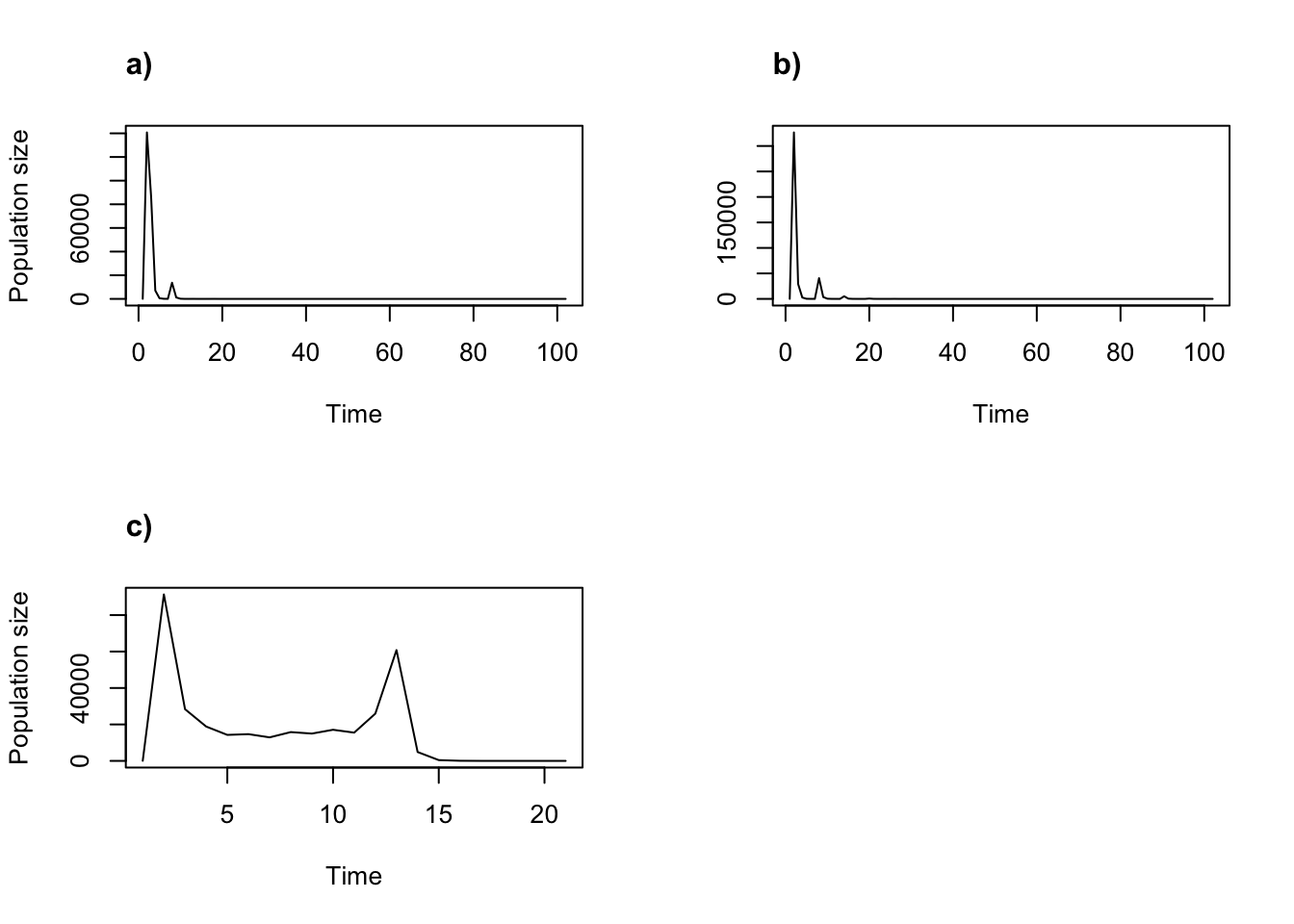
Figure 11.8: Cyclical and ordered density dependent function-based projections. (a) Cycle of all 6 year values for 101 years; (b) cycle of year values for 2005, 2006, and 2008 for 101 years; and (c) ordered progression for 20 years.
Cycling is obvious in the first two projections, and less so in the last.
As before, we can use density dependence in vital rates even with a cyclical or ordered simulation. In that circumstance, the density option simply needs to be replaced with an appropriate density_vr input (figure 11.9).
trial2f_18 <- f_projection3(data = cypfb_env, format = 3, stageframe = cypframe_fb,
  supplement = cypsupp2_fb, modelsuite = cypmodels2_env1, times = 20,
  year = year_order, ind_terms = mean_real, density_vr = vr1)
> Warning: Option patch not set, so will set to first patch/population.
> Warning: Too few values of individual covariates have been supplied. Some will
> be cycled.

plot(trial2f_18)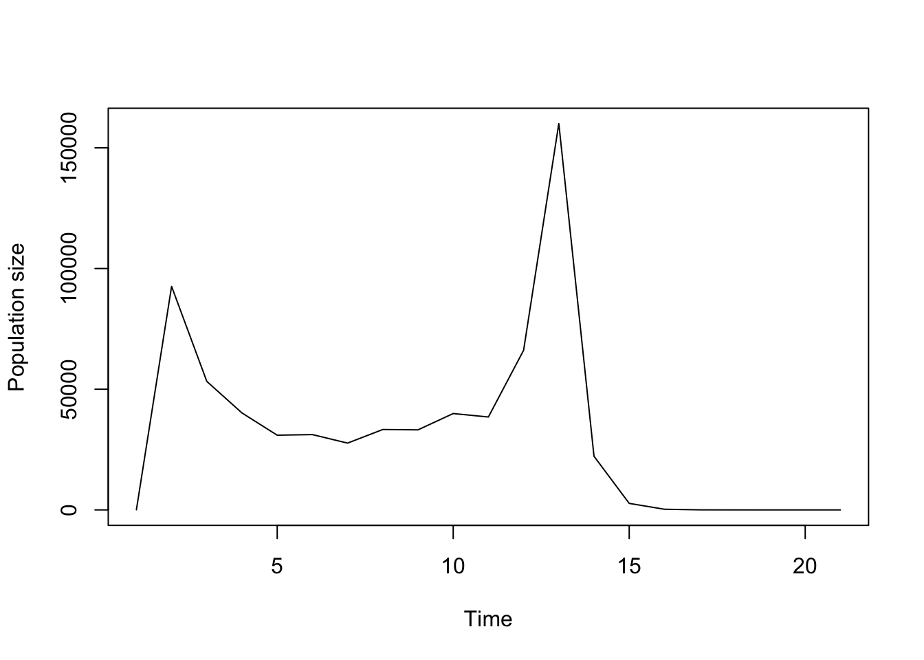
Figure 11.9: Ordered function-based projection with vital rate density dependence.
11.2.5 Replicated, density dependent simulations assuming temporal stochasticity using pre-existing MPMs
Finally, we may wish to conduct projections assuming both temporal stochasticity and density dependence. Here, we will set up four projections, each assuming one of four density frames with different parameterizations of the Ricker function working on germination (we have defined these density frames previously). We will assume that the choice of the next matrix does not depend on the current matrix.
set.seed(42)
cypproj2r_sd1 <- projection3(cypmatrix2r, stochastic = TRUE, times = 100,
  substoch = 2, density = c2d_1)

set.seed(42)
cypproj2r_sd2 <- projection3(cypmatrix2r, stochastic = TRUE, times = 100,
  substoch = 2, density = c2d_2)

set.seed(42)
cypproj2r_sd3 <- projection3(cypmatrix2r, stochastic = TRUE, times = 100,
  substoch = 2, density = c2d_3)

set.seed(42)
cypproj2r_sd4 <- projection3(cypmatrix2r, stochastic = TRUE, times = 100,
  substoch = 2, density = c2d_4)

summary(cypproj2r_sd1)
>
> The input lefkoProj object covers 1 population-patches.
> It is a single projection including 100 projected steps per replicate, and 1 replicates, respectively.
> The number of replicates with population size above the threshold size of 1 is as in
> the following matrix, with pop-patches given by column and milepost times given by row:
> $milepost_sums
>      1 1
> 0      1
> 0.25   1
> 0.5    1
> 0.75   1
> 1      1
>
> $extinction_times
> [1] NA

summary(cypproj2r_sd2)
>
> The input lefkoProj object covers 1 population-patches.
> It is a single projection including 100 projected steps per replicate, and 1 replicates, respectively.
> The number of replicates with population size above the threshold size of 1 is as in
> the following matrix, with pop-patches given by column and milepost times given by row:
> $milepost_sums
>      1 1
> 0      1
> 0.25   1
> 0.5    1
> 0.75   1
> 1      1
>
> $extinction_times
> [1] NA

summary(cypproj2r_sd3)
>
> The input lefkoProj object covers 1 population-patches.
> It is a single projection including 100 projected steps per replicate, and 1 replicates, respectively.
> The number of replicates with population size above the threshold size of 1 is as in
> the following matrix, with pop-patches given by column and milepost times given by row:
> $milepost_sums
>      1 1
> 0      1
> 0.25   1
> 0.5    1
> 0.75   1
> 1      1
>
> $extinction_times
> [1] NA

summary(cypproj2r_sd4)
>
> The input lefkoProj object covers 1 population-patches.
> It is a single projection including 100 projected steps per replicate, and 1 replicates, respectively.
> The number of replicates with population size above the threshold size of 1 is as in
> the following matrix, with pop-patches given by column and milepost times given by row:
> $milepost_sums
>      1 1
> 0      1
> 0.25   1
> 0.5    1
> 0.75   1
> 1      1
>
> $extinction_times
> [1] NA
Once again, let’s plot the projections for comparison (figure 11.10).
par(mfrow=c(2, 2))

plot(cypproj2r_sd1)
title("a)", adj = 0)

plot(cypproj2r_sd2, ylab = "")
title("b)", adj = 0)

plot(cypproj2r_sd3)
title("c)", adj = 0)

plot(cypproj2r_sd4, ylab = "")
title("d)", adj = 0)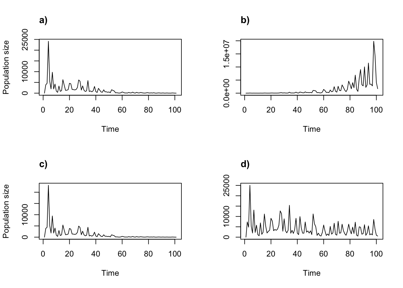
Figure 11.10: Stochastic density dependent projections assuming the two-parameter Ricker functon. (a) alpha = 0.05, beta = 0; (b) alpha = 1, beta = 0; (c) alpha = 0.05, beta = 0.0005; and (d) alpha = 1, beta = 0.0005.
We can clearly see the impact of temporal environmental stochasticity in each plot, and different density dependence relationships influence population trajectories strongly across the plots. Projections a) and c) appear to be moving to extinction, while projection b) is growing and projection d) appears to be fluctuating around some stable number. We can alter other settings, such as changing the weights of the matrices and using different density dependence relationships, as well as replicating our stochastic runs. Here, we re-run the first two projections with 100 replicates each and plot the results (figure 11.11).
set.seed(42)
cypproj2r_sd1_100 <- projection3(cypmatrix2r, stochastic = TRUE, times = 100,
  nreps = 100, substoch = 2, density = c2d_1)

set.seed(42)
cypproj2r_sd2_100 <- projection3(cypmatrix2r, stochastic = TRUE, times = 100,
  nreps = 100, substoch = 2, density = c2d_2)

par(mfrow = c(1, 2))

plot(cypproj2r_sd1_100)
title("a)", adj = 0)

plot(cypproj2r_sd2_100, ylab = "")
title("b)", adj = 0)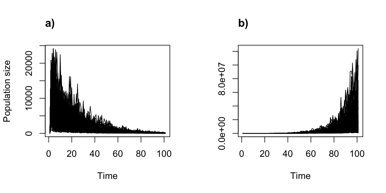
Figure 11.11: Stochastic density dependent projections with replicates assuming the two-parameter Ricker function. (a) alpha = 0.05, beta = 0; and (b) alpha = 1, beta = 0.
Note that each plot includes all replicates, each as a separate line. The general trends are the same as before, but we see the degree of variability in these trends is large.
We can also conduct density dependent discrete-state Markovian sequence-based analyses using these general projection functions. Let’s say that we wish to create a stochastic simulation using the state transition matrix state_mat, which we introduced in chapter 10. Let’s see that matrix again.
state_mat <- matrix(c(0.2, 0.2, 0.2, 0.2, 0.2, 0.1, 0.1, 0.6, 0.1, 0.1, 0.1,
    0.2, 0.4, 0.2, 0.1, 0.5, 0.4, 0.05, 0.05, 0, 0, 0, 0, 0.5, 0.5), ncol = 5)
state_mat
>      [,1] [,2] [,3] [,4] [,5]
> [1,]  0.2  0.1  0.1 0.50  0.0
> [2,]  0.2  0.1  0.2 0.40  0.0
> [3,]  0.2  0.6  0.4 0.05  0.0
> [4,]  0.2  0.1  0.2 0.05  0.5
> [5,]  0.2  0.1  0.1 0.00  0.5
Let’s now use our environmental state matrix as input in the tweights option, with stochastic = TRUE. Here, we will run a density independent projection first, followed by a density dependent sequence.
set.seed(42)
cyp_disc_proj1 <- projection3(mpm = cypmatrix2r, times = 100,
  tweights = state_mat, stochastic = TRUE, growthonly = FALSE)

set.seed(42)
cyp_disc_proj1_dens <- projection3(mpm = cypmatrix2r, times = 100,
  tweights = state_mat, stochastic = TRUE, growthonly = FALSE, density = c2d_1)

summary(cyp_disc_proj1)
>
> The input lefkoProj object covers 1 population-patches.
> It is a single projection including 100 projected steps per replicate, and 1 replicates, respectively.
> The number of replicates with population size above the threshold size of 1 is as in
> the following matrix, with pop-patches given by column and milepost times given by row:
> $milepost_sums
>      1 1
> 0      1
> 0.25   1
> 0.5    1
> 0.75   1
> 1      1
>
> $extinction_times
> [1] NA

summary(cyp_disc_proj1_dens)
>
> The input lefkoProj object covers 1 population-patches.
> It is a single projection including 100 projected steps per replicate, and 1 replicates, respectively.
> The number of replicates with population size above the threshold size of 1 is as in
> the following matrix, with pop-patches given by column and milepost times given by row:
> $milepost_sums
>      1 1
> 0      1
> 0.25   1
> 0.5    1
> 0.75   1
> 1      1
>
> $extinction_times
> [1] NA
Let’s plot the two projections (figure 11.12).
par(mfrow = c(1, 2))

plot(cyp_disc_proj1)
title("a)", adj = 0)

plot(cyp_disc_proj1_dens)
title("b)", adj = 0)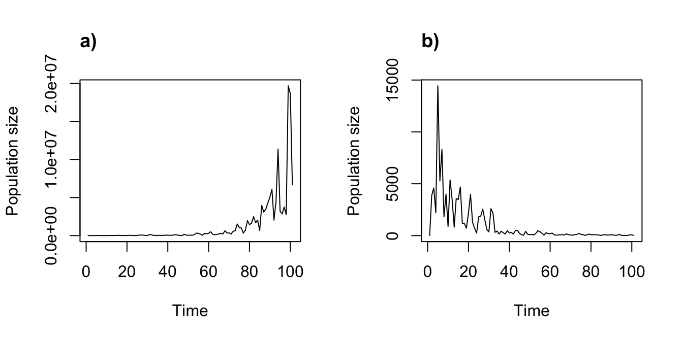
Figure 11.12: Density independent vs. density dependent projections assuming discrete-state Markovian temporal stochasticity.
The approach just described provides us with a single stochastic run in each case. Let’s now try replicating, as we might typically do in a stochastic analysis. Let’s redo the above projections, but with 100 replicates each, and plot the results (figure 11.13).
set.seed(42)
cyp_disc_proj1_100 <- projection3(mpm = cypmatrix2r, times = 100, nreps = 100,
  tweights = state_mat, stochastic = TRUE, growthonly = FALSE)

set.seed(42)
cyp_disc_proj1_dens_100 <- projection3(mpm = cypmatrix2r, times = 100,
  nreps = 100, tweights = state_mat, stochastic = TRUE, growthonly = FALSE,
  density = c2d_1)

par(mfrow = c(1, 2))

plot(cyp_disc_proj1_100)
title("a)", adj = 0)

plot(cyp_disc_proj1_dens_100)
title("b)", adj = 0)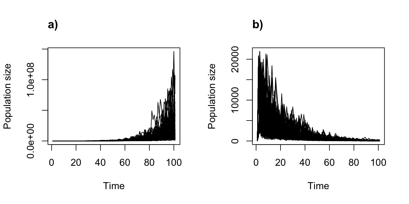
Figure 11.13: Density independent vs. density dependent projections assuming discrete-state Markovian temporal stochasticity, with 100 replicates each.
Voilà!
11.2.6 Replicated function-based projection assuming temporal stochasticity and density dependence
Finally, we might conduct a density dependent function-based stochastic projection. In this case, we will probably wish to run a simulation with replicates. Here is one such projection using one of our previous density frames.
set.seed(42)
trial2f_19 <- f_projection3(data = cypfb_env, format = 3, stochastic = TRUE,
  substoch = 2, stageframe = cypframe_fb, supplement = cypsupp2_fb,
  modelsuite = cypmodels2_env1, times = 101, nreps = 100,
  ind_terms = mean_real, density = c2d)
Let’s look at a summary of the projection.
summary(trial2f_19)
>
> The input lefkoProj object covers 1 population-patches.
> It is a single projection including 101 projected steps per replicate, and 100 replicates, respectively.
> The number of replicates with population size above the threshold size of 1 is as in
> the following matrix, with pop-patches given by column and milepost times given by row:
> $milepost_sums
>      1 1
> 0    100
> 0.25 100
> 0.5  100
> 0.75 100
> 1    100
>
> $extinction_times
> [1] NA
Here is one further such projection, using a different density dependence relationship.
c2d1 <- density_input(cyp_ex, stage3 = c("P1", "P1"),
  stage2 = c("SD", "rep"), style = 1, time_delay = 1, alpha = 2, beta = 0.5,
  type = c(2, 2))

trial2f_20 <- f_projection3(data = cypfb_env, format = 3, stochastic = TRUE,
  substoch = 2, stageframe = cypframe_fb, supplement = cypsupp2_fb,
  modelsuite = cypmodels2_env1, times = 101, nreps = 100,
  ind_terms = mean_real, density = c2d1)
Let’s see a summary.
summary(trial2f_20)
>
> The input lefkoProj object covers 1 population-patches.
> It is a single projection including 101 projected steps per replicate, and 100 replicates, respectively.
> The number of replicates with population size above the threshold size of 1 is as in
> the following matrix, with pop-patches given by column and milepost times given by row:
> $milepost_sums
>      1 1
> 0    100
> 0.25 100
> 0.5  100
> 0.75 100
> 1    100
>
> $extinction_times
> [1] NA
Let’s take a peek at what the results look like (figure 11.14).
par(mfrow = c(1, 2))

plot(trial2f_19)
title("a)", adj = 0)

plot(trial2f_20, ylab = "")
title("b)", adj = 0)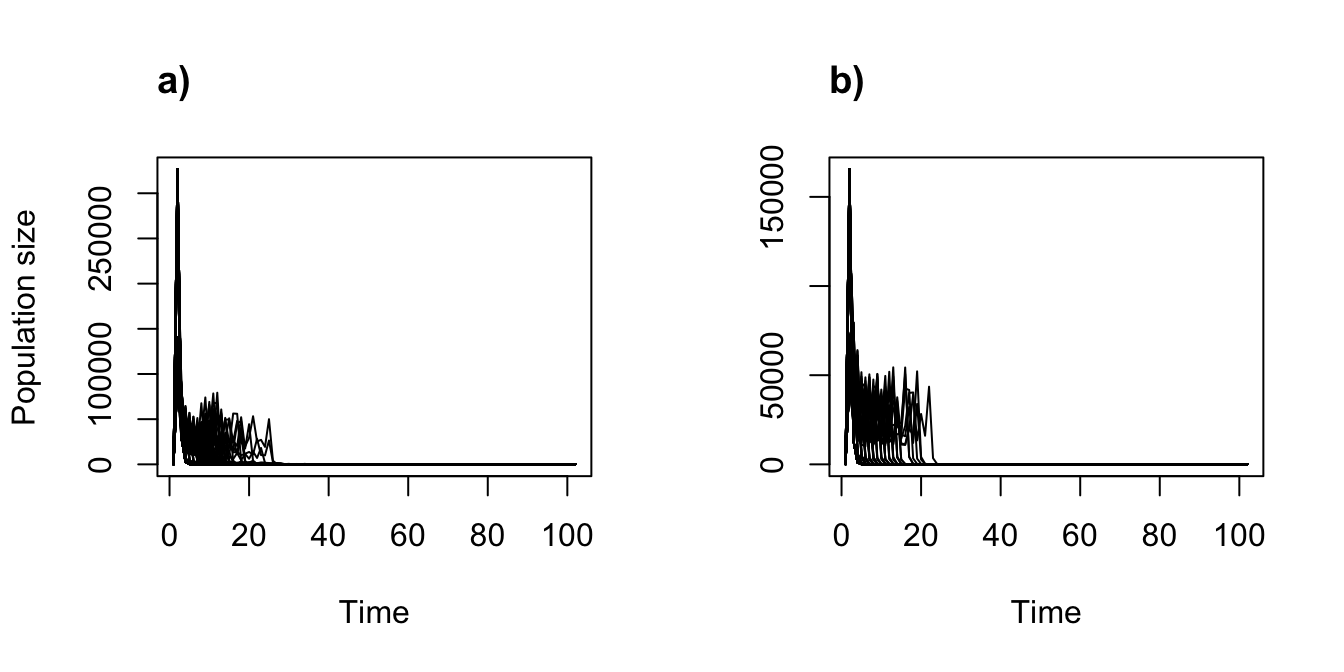
Figure 11.14: Stochastic density dependent function-based projections, assuming two different sets of values for the Ricker function.
The different values of the Ricker function have not yielded dramatic differences here, although looking through the pop_size elements of each simulation will reveal large differences in predicted population size across years. We encourage the user to experiment further with different settings.
As with projection3(), we can use function f_projection3() to run discrete-state Markovian temporally stochastic projections. Here, we use the environmental state transition matrix state_mat to create such an analysis. Let’s try a single replicate first. We will also plot the result (figure 11.15).
trial2f_21_1 <- f_projection3(data = cypfb_env, format = 3, stochastic = TRUE,
  substoch = 2, stageframe = cypframe_fb, supplement = cypsupp2_fb,
  modelsuite = cypmodels2_env1, times = 101, nreps = 1,
  ind_terms = mean_real, density = c2d1, tweights = state_mat)
> Warning: Option patch not set, so will set to first patch/population.
> Warning: Too few values of individual covariates have been supplied. Some will
> be cycled.

plot(trial2f_21_1)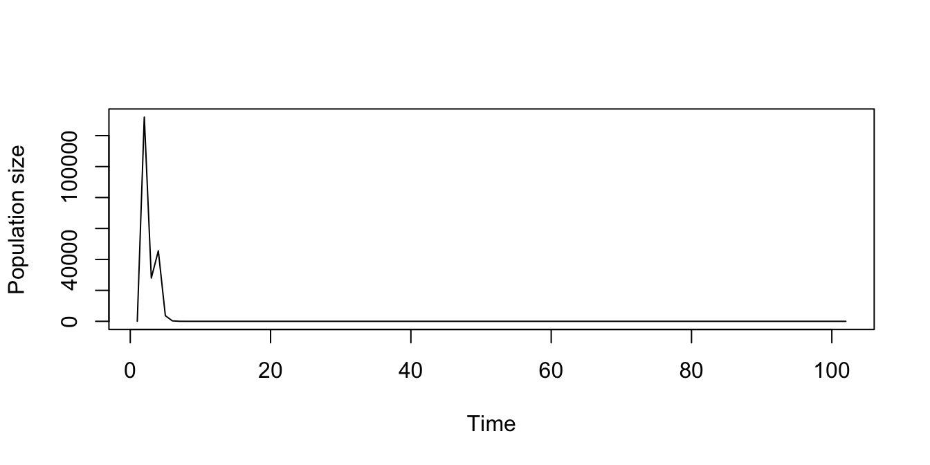
Figure 11.15: Stochastic density dependent function-based projection, assuming a discrete-state Markovian sequence of matrices.
Let’s repeat, but with 100 replicates now. Note that the following block will likely take a while to run. Go and get yourself a cappuccino while you wait….
trial2f_21_100 <- f_projection3(data = cypfb_env, format = 3, stochastic = TRUE,
  substoch = 2, stageframe = cypframe_fb, supplement = cypsupp2_fb,
  modelsuite = cypmodels2_env1, times = 101, nreps = 100,
  ind_terms = mean_real, density = c2d1, tweights = state_mat)
Let’s see a summary.
summary(trial2f_21_100)
>
> The input lefkoProj object covers 1 population-patches.
> It is a single projection including 101 projected steps per replicate, and 100 replicates, respectively.
> The number of replicates with population size above the threshold size of 1 is as in
> the following matrix, with pop-patches given by column and milepost times given by row:
> $milepost_sums
>      1 1
> 0    100
> 0.25 100
> 0.5  100
> 0.75 100
> 1    100
>
> $extinction_times
> [1] NA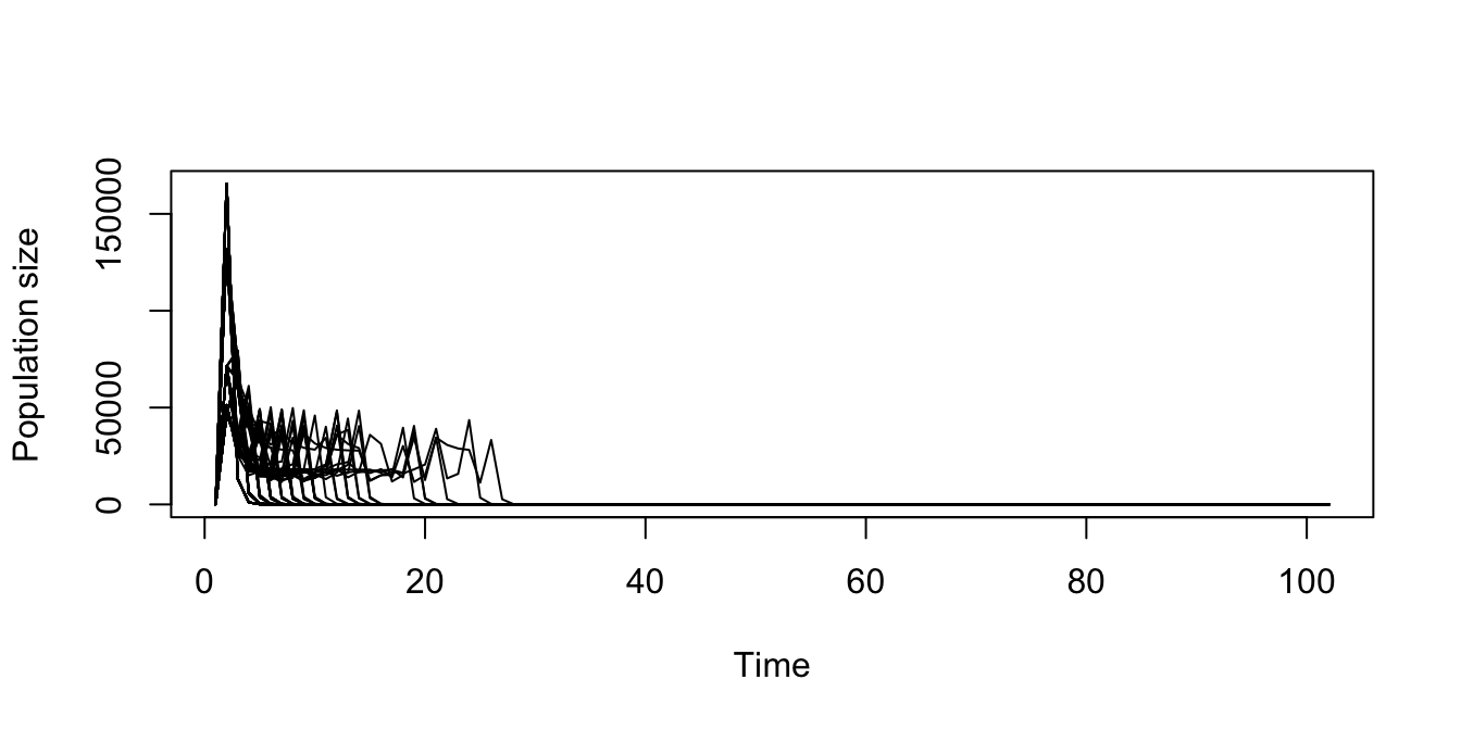
Figure 11.16: Replicated stochastic density dependent function-based projection, assuming a discrete-state Markovian sequence of matrices.
Voilà!
11.3 Weighting stages
Density dependence can vary greatly across organisms. Different scenarios might require different functions, such as the Ricker or Beverton-Holt, applied with different values to different elements or vital rates. Likewise, there may also be situations in which different stages likely have a different influence on the density dependence function. For this purpose, lefko3 allows the use of stage weights in density dependence projections.
Stage weights are multipliers on the numbers of individuals in each stage at each time, used to determine the number to fix as the density responded to in that time by density dependence functions. An extreme example from the plant literature might illustrate the problem. In the case of the orchid Cypripedium candidum, reproductive individuals produce many thousands of dust seeds per reproductive episode. These dust seeds may germinate by the time of the next growing season, they may die, or they may remain dormant. Adding the numbers of dormant seeds, or even of just germinated protocorms, would inflate the population greatly. There may be reason to do so, but in this case, it is very likely that dormant seeds have no impact on the response of other individuals to density, and it is even likely that 1st year protocorms have little to no influence on this, as well. Thus, in this specific case, we might use a stage weight of 0 for dormant seeds, and either 0 or a small number for 1st year protocorms. All other stages would be left having a default stage weight of 1.
Here is an example in action. Let’s first create a new data frame of class lefkoEq, using the stage_weight() function, to set stage weights that will not equal 1.
cyp_weights <- stage_weight(cypmatrix2r, stage2 = c("SD", "P1"), value = c(0., 0.1))

cyp_weights
>   stage2 stage_id_2 stage1 stage_id_1 age2 row_num value
> 1     SD          1     NA         NA   NA       1   0.0
> 2     P1          2     NA         NA   NA       2   0.1
Let’s now apply our stage weights to one of our previous projections, and look at the difference (figure 11.17).
cypproj2_d4_weighted <- projection3(cypmean2, times = 100, substoch = 2,
  density = c2d_4, stage_weights = cyp_weights)
> Warning: This lefkoMat object appears to be a set of mean matrices. Will
> project only the mean.

par(mfrow = c(1, 2))

plot(cypproj2_d4)
plot(cypproj2_d4_weighted)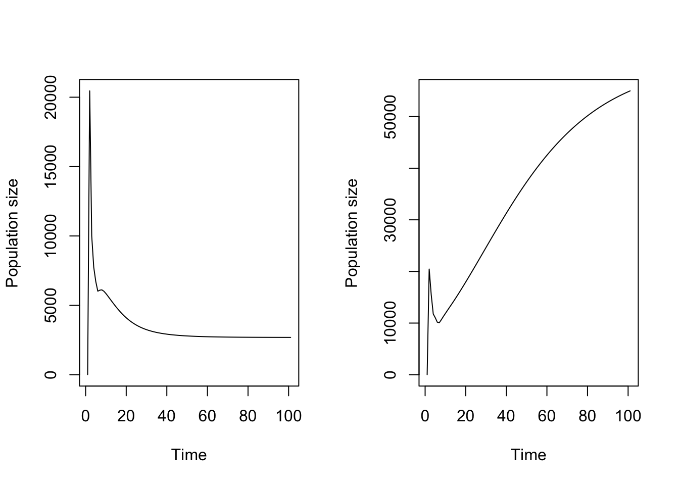
Figure 11.17: Projection assuming a) all stages contribute equally to density, and b) dormant seed do not contribute while 1st year protocorms only slightly contribute to density
We see some clear differences here, although they are not always guaranteed. Let’s now look at a function-based version (figure 11.18).
trial2f_16_weighted <- f_projection3(data = cypfb_env, format = 3,
  stageframe = cypframe_fb, supplement = cypsupp2_fb,
  modelsuite = cypmodels2_env1, times = 101, year = c(2005, 2006, 2008),
  ind_terms = mean_real, density = c2d, stage_weights = cyp_weights)
> Warning: Option patch not set, so will set to first patch/population.
> Warning: Too few values of individual covariates have been supplied. Some will
> be cycled.

par(mfrow = c(1, 2))

plot(trial2f_16)
plot(trial2f_16_weighted)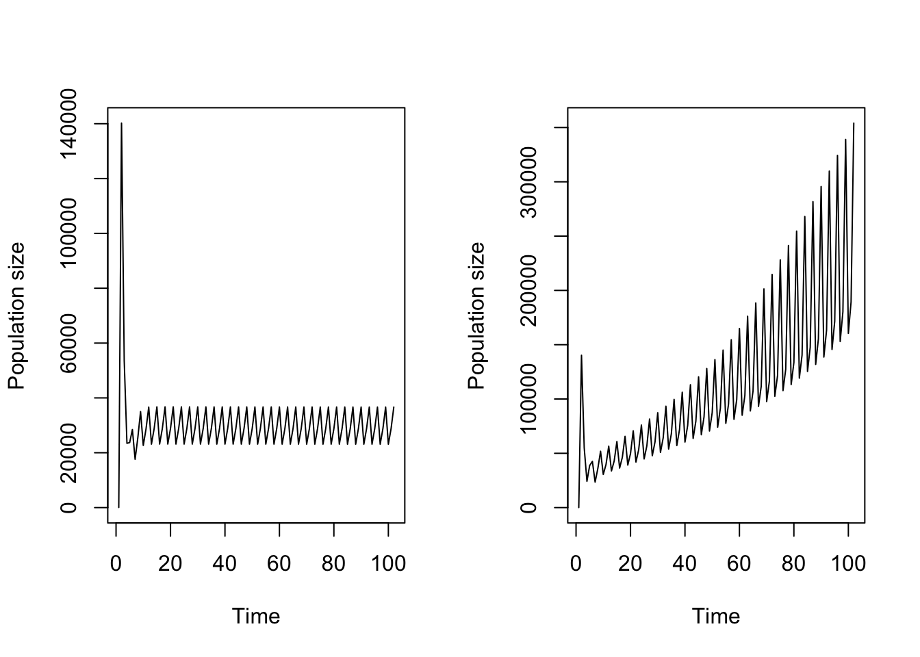
Figure 11.18: Function-based projection assuming a) all stages contribute equally to density, and b) dormant seed do not contribute while 1st year protocorms only slightly contribute to density
Stage weights can be any non-negative value. Users are encouraged to experiment!
11.4 Bootstrapping with density dependence
As with all cases up to this point, density dependence can be applied in bootstrapped projections, and using the same approaches that we have seen up to this point. Let’s conduct a projection of pre-existing bootstrapped MPMs, as below. We will create a new bootstrapped version of the stage weighted projection above.
set.seed(42)

cypraw_v1_boot <- bootstrap3(cypraw_v1, reps = 3)

cypmatrix2r_boot <- rlefko2(data = cypraw_v1_boot, stageframe = cypframe_raw,
  year = "all", stages = c("stage3", "stage2"),
  size = c("size3added", "size2added"), supplement = cypsupp2_raw,
  yearcol = "year2", indivcol = "individ")

cypmean2_boot <- lmean(cypmatrix2r_boot)

cypproj2_d4_weighted_boot <- projection3(cypmean2_boot, times = 100,
  substoch = 2, density = c2d_4, stage_weights = cyp_weights)
> Warning: This lefkoMat object appears to be a set of mean matrices. Will
> project only the mean.
> Warning: This lefkoMat object appears to be a set of mean matrices. Will
> project only the mean.
> Warning: This lefkoMat object appears to be a set of mean matrices. Will
> project only the mean.

summary(cypproj2_d4_weighted_boot)
>      Length Class     Mode
> [1,] 10     lefkoProj list
> [2,] 10     lefkoProj list
> [3,] 10     lefkoProj list
We see that we have created a list of lefkoProj objects, known as an object of class lefkoProjList. Let’s now plot these 3 against the original, unbootstrapped projection.
par(mfrow = c(2, 2))

plot(cypproj2_d4_weighted)
plot(cypproj2_d4_weighted_boot[[1]])
plot(cypproj2_d4_weighted_boot[[2]])
plot(cypproj2_d4_weighted_boot[[3]])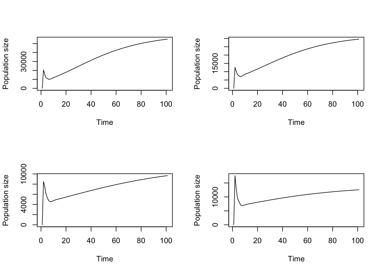
Figure 11.19: Comparison of a) original, stage weighted projection against b-d) bootstrapped versions of the same projection
We see some interesting differences driven by differences among individuals.
What about the function-based case? It is exactly the same as before. Let’s start off by bootstrapping the original function-based version of the dataset.
set.seed(42)

cypfb_env_boot <- bootstrap3(cypfb_env, reps = 3)

summary_hfv(cypfb_env_boot)
>
> This hfvlist object contains 3 hfvdata demographic data frames.
> Each data frame contains an average of 306.333 rows, 60 variables, 1 population,
> 3 patches, 44.667 individuals, and 5 time steps.
>
> Across all data frames, there are 1 unique population, 3 unique patches, 72 unique individuals, and 5 unique time steps.
Now we will create modelsuites for our bootstrapped data.
cypmodels2_env_boot <- modelsearch(cypfb_env_boot, historical = FALSE,
  approach = "mixed", vitalrates = c("surv", "obs", "size", "repst", "fec"),
  sizedist = "negbin", size.trunc = TRUE, fecdist = "poisson", fec.zero = TRUE,
  suite = "main", size = c("size3added", "size2added", "size1added"),
  indcova = c("indcova3", "indcova2", "indcova1"), test.indcova = TRUE,
  quiet = "partial")
And now the summary.
summary(cypmodels2_env_boot)
>      Length Class    Mode
> [1,] 31     lefkoMod list
> [2,] 31     lefkoMod list
> [3,] 31     lefkoMod list
Let’s now build the projections! Let’s try doing bootstrapped versions of the stage-weighted projections above.
trial2f_16_weighted_boot <- f_projection3(data = cypfb_env_boot, format = 3,
  stageframe = cypframe_fb, supplement = cypsupp2_fb,
  modelsuite = cypmodels2_env_boot, times = 101, year = c(2005, 2006, 2008),
  ind_terms = mean_real, density = c2d, stage_weights = cyp_weights)
> Warning: Option patch not set, so will set to first patch/population.
> Warning: Too few values of individual covariates have been supplied. Some will
> be cycled.
> Warning: Option patch not set, so will set to first patch/population.
> Warning: Too few values of individual covariates have been supplied. Some will
> be cycled.
> Warning: Option patch not set, so will set to first patch/population.
> Warning: Too few values of individual covariates have been supplied. Some will
> be cycled.

summary(trial2f_16_weighted_boot)
>      Length Class     Mode
> [1,] 11     lefkoProj list
> [2,] 11     lefkoProj list
> [3,] 11     lefkoProj list
Finally, let’s plot the original against our 3 bootstraps and see what happened (figure 11.20).
par(mfrow = c(2, 2))

plot(trial2f_16_weighted)
plot(trial2f_16_weighted_boot[[1]])
plot(trial2f_16_weighted_boot[[2]])
plot(trial2f_16_weighted_boot[[3]])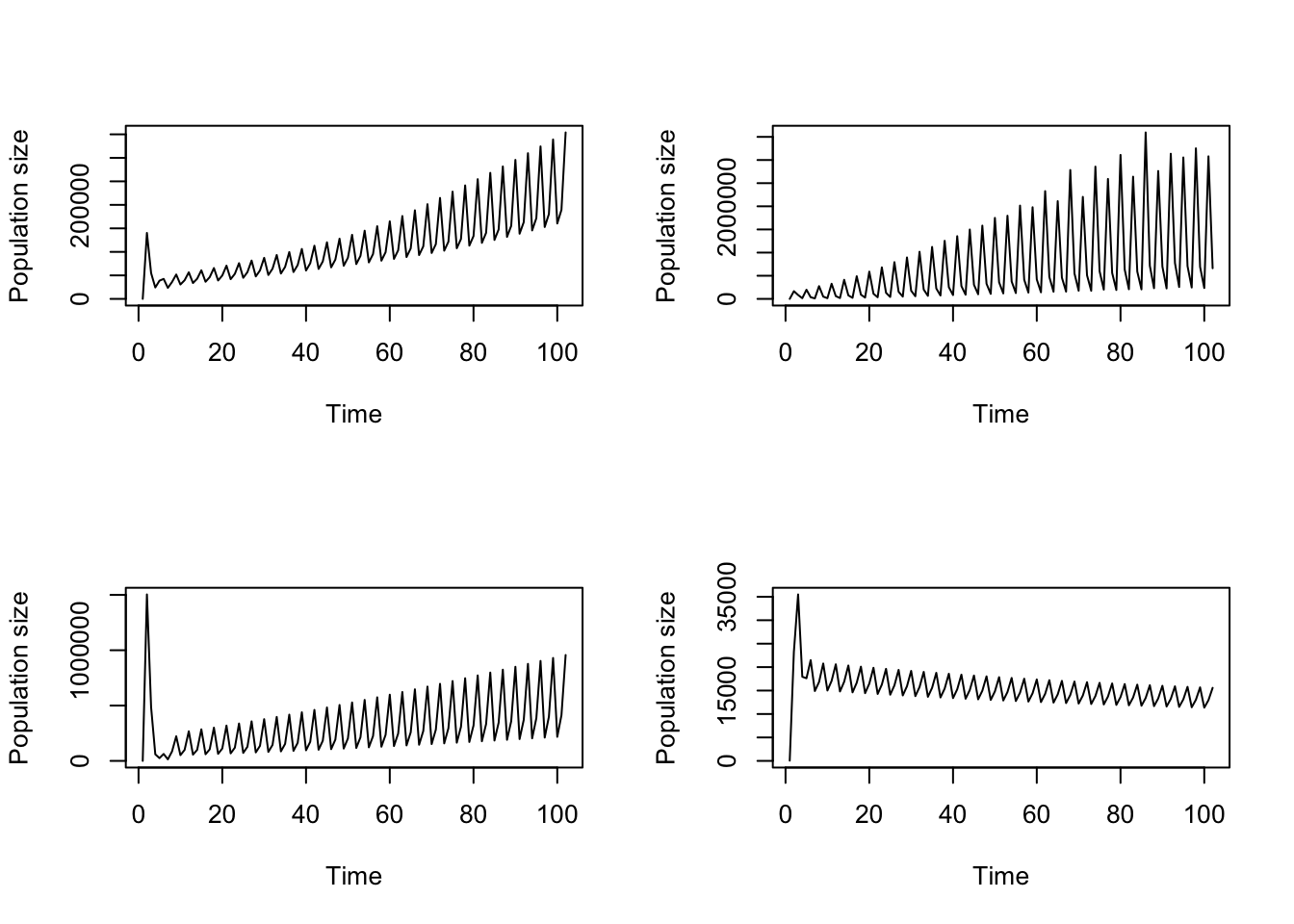
Figure 11.20: Comparison of a) original, stage weighted function-based projection against b-d) bootstrapped versions of the same projection
Some really fascinating results driven by individual differences, yet again!
11.5 Points to remember
- Both projection functions include two substochasticity settings that can prevent impossible values, such as negative fecundity or survival probability above 1.0, from being incorporated into matrix projection.
- Users may set density dependence in matrix elements or in vital rates, using the
density_input()anddensity_vr()functions, respectively.
- Density dependence can be set with discrete-state Markovian stochastic environmental sequences, even with replication.
- Stages can be weighted differently against the density values used in density dependence functions, using function
stage_weight(). - Density dependent projections can be bootstrapped, in the same ways that MPMs can be bootstrapped in
lefko3.