2.4 Creating Tables
To make working with data easier, you can organize data in a table format on a worksheet.
You are going to use Excel’s random number generator and tables to create a fictional grade book.
2.4.1 Practice 2
- Select the block of cells D1:H11.
- On the
Hometab, in theStylesribbon, clickFormat as Table, and then click the table style of your choice.
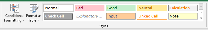
Figure 2.9: Style ribbon.
- Select the
My table has headerscheck box in theFormat as Tabledialog window.
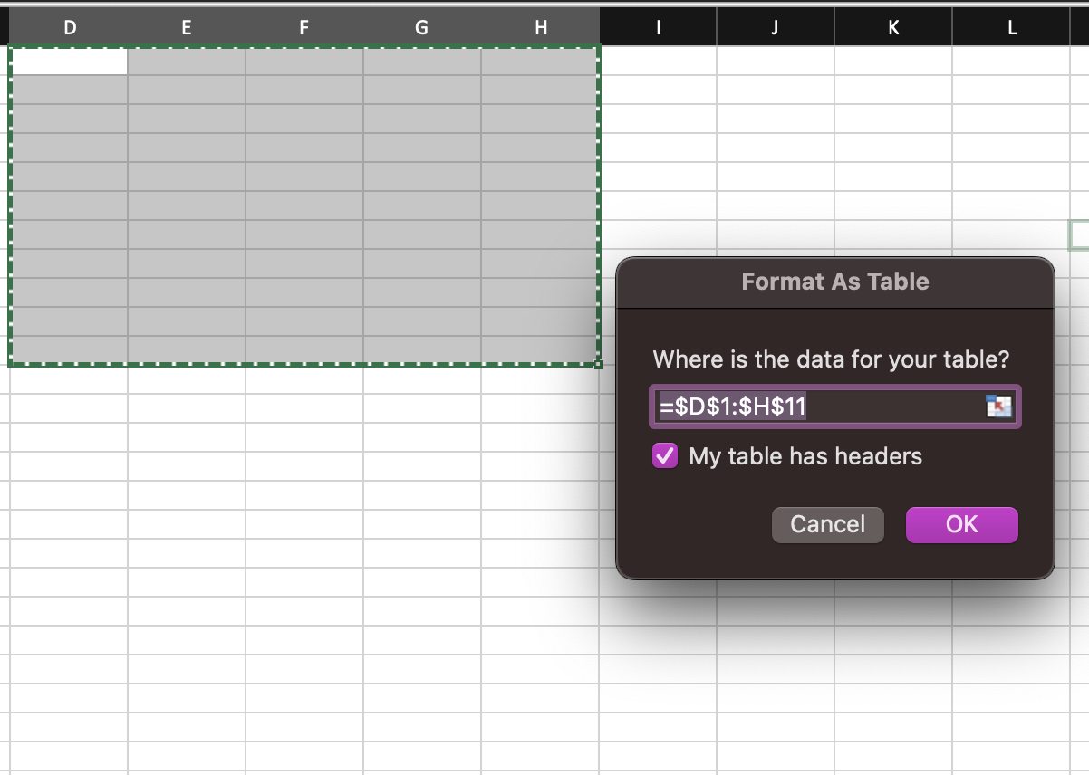
Figure 2.10: 32: Format As Table window.
Note: When you select a table by clicking the mouse pointer, the Table Tools menu becomes available, and a Design tab is displayed. To get a good idea of what you can add to or change in your table, click the Design tab, then explore the groups and options provided on this tab.
- Replace the table headers. Instead of
Columns1throughColumn5, replace headers by typing in them the following: Name, Exam 1, Exam 2, Exam 3 and Final Exam. - Under header Name, in cells 2-11, create 10 students’ names, writing last name, and first name.
- Now select the block of cells D2:D11. Click
Home > Sort & Filter > Select A to Z. The fictional names should then appear in alphabetical order. - Select cell E2. Click on the
Formulabar, type in=RANDBETWEEN(0,100). - Position the mouse pointer in the lower right corner of cell E2 until it becomes a
+sign and click-drag downward until you reach cell E11. Release (Note: Sometimes this feature is not needed within a formatted table). - Repeat the process above for Column F using
=RANDBETWEEN(40,98). - Repeat the process above for Column G using
=RANDBETWEEN(64,105). - Repeat the process above for Column H using
=RANDBETWEEN(37,100). - If the list of numbers is not randomized, click the button
Calculate Now.