1.8 Arithmetic Options on the Standard Toolbar
1.8.1 Sum Function
On the Formula Menu, the button you see in Figure 1.21 automatically sums the values in the selected cells.

Figure 1.21: Autosum button.
When we sum the contents of an entire column, Excel places the sum under the selected cells. It is a good idea to type the label Total next to the cell where the total appears.
1.8.2 Practice 2
For the data you entered in your worksheet (see Practice 1), select cells in Column A containing numerical values (a2:a21). Press the button AutoSum, then type the word Total in the corresponding row of Column C. We see that the sum of Column A is 419.
1.8.3 Sorting Data
The Sort and Filter ribbon on the Home tab shown in Figure 1.22 can be used to sort the data in ascending or descending depending on the selection from the sub-menu.
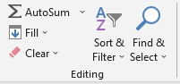
Figure 1.22: Sort and Filter buttons.
To sort just one column, highlight that column and press the button and select the sort order. To sort two or more columns by ascending or descending order of the data in the first column, highlight all the columns and click the appropriate button. In general, we will sort one column of data.
1.8.4 Practice 3
- Sort the data in the first column in ascending order.
- Now undo the ordering you just did to your data.
– If you have not made any other changes since you did the sort, you can use
Undofunction of Excel from theTitle Barfrom the main menu. The data will appear in their original order. – Another option to undo actions in Excel, use the keysCRTL-Zon a PC keyboard orCommand-Zon a MAC.
After Step 2 above, your data set should be in the original form.
1.8.5 Copying Cells
To copy one cell or a block of cells to another location on the worksheet:
- Select the cells you wish to copy.
- From the
Hometab, selectCopy(the shortcut with the keyboard for this process isCRTL-Con PC orCommand-Con MAC). Notice that the range of cells being copied now has a blinking border around it. - Select the upper-left cell of the block that will receive the copy.
- Press Enter. When you press Enter, the copy process is complete, and the blinking border around the original cells disappears.
Note: Even if you use the command Paste or the shortcut CRTL-V on PC or Command-V on MAC to paste, you must still press Enter to remove the blinking border around the original cells. To copy one cell or a range of cells to another worksheet or workbook, follow Steps 1 and 2 above. For Step
3, be sure you are in the destination worksheet or workbook and that the worksheet or workbook is activated. Then proceed to Step 4.
1.8.6 Practice 4
- Copy the contents of columns A and B and paste them into columns F and G. Then sort the data in Column F in descending order
- Also, copy the contents of columns A and B and paste them into columns J and K. Then custom sort the data in Columns J and K by the values in Column J in ascending order
After Step 2 above, your worksheet should have 3 sets of data where the two (2) rightmost ones have modifications in the ordering of the columns according to the instructions in the practice above.