B Remuestreo
Paquetes de esta sección
B.1 Bootstrap
B.1.1 El Principio Bootstrap
Recrear la relación entre la población y la muestra, considerando la muestra como un epítome de la población subyacente, y por remuestreo de ella (adecuadamente), generar la muestra bootstrap, que sirve como un análogo de la muestra dada.
Si el mecanismo de remuestreo se elige apropiadamente, entonces se espera que el remuestreo, junto con la muestra en cuestión, reflejen la relación original entre la población y la muestra.
La ventaja es que ahora se puede evitar el problema de tener que lidiar con la población, y en su lugar, se utilice la muestra y los remuestreos, para abordar cuestiones de inferencia estadística con respecto a las cantidades desconocidas de la población.
El principio de bootstrap aborda el problema de no tener un conocimiento completo de la población, para hacer inferencia acerca del estimador \(\hat{\theta}\).
El primer paso consiste en la construcción de un estimador de \(\mathcal{F}(\hat{\mathcal{F}})\) desde las observaciones disponibles \(X_1\ldots X_n\), el cual proporciona una imagen representativa de la población.
El siguiente paso consiste en la generación de variables aleatorias i.i.d. \(X_1^{*}\ldots X_n^{*}\) del estimador \(\hat{\mathcal{F}}\) (condicionada a las observaciones \(\mathcal{X}_n\)), el cual cumple el rol de la muestra para la versión bootstrap del problema original.
Por lo tanto, la versión bootstrap del estimador \(\hat{\theta}\) basado en la muestra original \(X_1\ldots X_n\) está dada por \(\hat{\theta}^{*}\), obtenido mediante la sustitución de \(X_1\ldots X_n\) por \(X_1^{*}\ldots X_n^{*}\).
B.1.2 Tipos de bootstrap
Paramétrico: Si se supone que $\mathcal{F}$ pertenece a un modelo paramétrico $\mathcal{F}_{\theta}: \theta \in \Theta$, entonces, $\mathcal{F} = \mathcal{F}_{\hat{\theta}}$, donde $\hat{\theta}$ es un estimador de $\theta$.No paramétrico: Si no se hace ninguna hipótesis sobre $\mathcal{F}$, entonces, $\hat{\mathcal{F}} = \hat{\mathcal{F}}_{n}$, donde $\hat{\mathcal{F}}_{n}$ es la función de distribución empírica.
Método plug-in: Si se desea estimar una cantidad \(\theta = T(\mathcal{F})\), que depende de la función de distribución \(\mathcal{F}\) de los datos, el método plug-in (o sustitución), \[ \hat{\theta} = T(\hat{\mathcal{F}_n}); \] donde F es sustituido por la función de distribución empírica \(\hat{\mathcal{F}_n}\).
Función de distribución empírica (\(\hat{\mathcal{F}_n}\)): La \(\hat{\mathcal{F}_n}\) de la m.a.(\(n\)), asigna probabilidad \(\frac{1}{n}\) a cada valor \(X_i\) con \(i = 1,\ldots,n\), \[ \hat{\mathcal{F}_n} = \frac{1}{n}\sum_{i = 1}^{n} \mathbb{I}(X_i\leq x_i) \] donde \(\mathbb{I}\) es la función indicatriz.
B.1.3 Bootstrap para datos i.i.d.
Desarrollado por Efron (1979), también llamada bootstrap ordinario. Sirve para estimar o aproximar la distribución del estadístico y sus características.
Asume que \(\mathcal{F}\) es la F.D. de una muestra \(\mathbf{X}_n = (X_1\ldots,X_n)^T\) y se quiere estudiar un estadístico \(T_n = t_n(\mathbf{X}_n,\mathcal{F})\) y sus características (sesgo, varianza, error estándar, etc.).
En el método bootstrap, se va a fabricar versiones bootstrap de \(T_n\) utilizando la misma forma funcional sustituyendo \(\mathcal{F}\) por \(\hat{\mathcal{F}}_n\), y la muestra \(\mathbf{X}_n\) por muestras con distribución \(\hat{\mathcal{F}}_n\) en vez de \(\mathcal{F}\).
De esta manera a partir de la muestra dada \(\mathbf{X}_n = (X_1\ldots,X_n)^T\) , se selecciona una muestra aleatoria simple \(\mathbf{X}_m^{*} = (X_1^{*}\ldots,X_m^{*})^T\) de tamaño \(m\) con reemplazo de \(\mathbf{X}_n\), llamada muestra bootstrap. Así, son variables aleatorias i.i.d., con distribución \(\hat{\mathcal{F}}_n\).
B.1.4 Ejemplo
set.seed(23434)
x1 <- rnorm(40,0,1)
x2 <- rnorm(40,0,1)
y <- 10 + x1*2 - 5*x2 + rnorm(40,0,1)

reg.1 <- lm(y ~ x1 + x2)
summary(reg.1)
##
## Call:
## lm(formula = y ~ x1 + x2)
##
## Residuals:
## Min 1Q Median 3Q Max
## -1.80172 -0.77731 -0.02077 0.77349 1.67730
##
## Coefficients:
## Estimate Std. Error t value Pr(>|t|)
## (Intercept) 10.0211 0.1589 63.07 <2e-16 ***
## x1 1.9965 0.1339 14.91 <2e-16 ***
## x2 -4.8735 0.1507 -32.33 <2e-16 ***
## ---
## Signif. codes: 0 '***' 0.001 '**' 0.01 '*' 0.05 '.' 0.1 ' ' 1
##
## Residual standard error: 0.996 on 37 degrees of freedom
## Multiple R-squared: 0.9724, Adjusted R-squared: 0.9709
## F-statistic: 652.3 on 2 and 37 DF, p-value: < 2.2e-16Ahora usamos el paquete boot.
Definimos el conjunto de datos:
Intentemos calcular intervalos de confianza del \(95\%\). El paquete bootstrap funciona escribiendo primero una función para llamar a los resultados de regresión, luego ejecutando el comando boot y luego analizando los resultados. Llamaremos a nuestro programa para buscar nuestra estadístico bootstrap:
bootstrap <- function(formula, data, regressors) {
    dat <- data[regressors,]    # obtiene la muestra
    reg <- lm(formula, data = dat) # corre la regresión
    return(coef(reg)) # necesitamos estos coeficientes
}
Ahora ejecutamos un gran número de repeticiones (normalmente 1000 o más) en nuestra regresión con my.data, y obtenemos el estadístico boot escrita anteriormente
bs.res <- boot(R = 1000, formula = y~x1 + x2 , data = my.data, statistic = bootstrap)
print(bs.res)  # nota que todo se graba
##
## ORDINARY NONPARAMETRIC BOOTSTRAP
##
##
## Call:
## boot(data = my.data, statistic = bootstrap, R = 1000, formula = y ~
## x1 + x2)
##
##
## Bootstrap Statistics :
## original bias std. error
## t1* 10.021085 -0.000352671 0.1604612
## t2* 1.996487 -0.005474321 0.1516179
## t3* -4.873461 -0.010313515 0.1339507Con la función boot.ci, podemos llamar a 5 tipos diferentes de salidas de intervalo de confianza para usar. A continuación se presentan cuatro de ellos. Tenga en cuenta que llamaré al índice de los resultados:
## (Intercept)          x1          x2
##   10.021085    1.996487   -4.873461
Bootstrap básico
## BOOTSTRAP CONFIDENCE INTERVAL CALCULATIONS
## Based on 1000 bootstrap replicates
##
## CALL :
## boot.ci(boot.out = bs.res, type = "basic", index = 2)
##
## Intervals :
## Level      Basic
## 95%   ( 1.712,  2.298 )
## Calculations and Intervals on Original Scale## BOOTSTRAP CONFIDENCE INTERVAL CALCULATIONS
## Based on 1000 bootstrap replicates
##
## CALL :
## boot.ci(boot.out = bs.res, type = "basic", index = 3)
##
## Intervals :
## Level Basic
## 95% (-5.101, -4.588 )
## Calculations and Intervals on Original ScalePercentiles bootstrap (BCa)
## BOOTSTRAP CONFIDENCE INTERVAL CALCULATIONS
## Based on 1000 bootstrap replicates
##
## CALL :
## boot.ci(boot.out = bs.res, type = "bca", index = 2)
##
## Intervals :
## Level BCa
## 95% ( 1.731, 2.335 )
## Calculations and Intervals on Original Scale## BOOTSTRAP CONFIDENCE INTERVAL CALCULATIONS
## Based on 1000 bootstrap replicates
##
## CALL :
## boot.ci(boot.out = bs.res, type = "bca", index = 3)
##
## Intervals :
## Level BCa
## 95% (-5.145, -4.640 )
## Calculations and Intervals on Original Scale## BOOTSTRAP CONFIDENCE INTERVAL CALCULATIONS
## Based on 1000 bootstrap replicates
##
## CALL :
## boot.ci(boot.out = bs.res, type = "bca", index = 3)
##
## Intervals :
## Level BCa
## 95% (-5.145, -4.640 )
## Calculations and Intervals on Original ScaleNormal
## BOOTSTRAP CONFIDENCE INTERVAL CALCULATIONS
## Based on 1000 bootstrap replicates
##
## CALL :
## boot.ci(boot.out = bs.res, type = "norm", index = 2)
##
## Intervals :
## Level Normal
## 95% ( 1.705, 2.299 )
## Calculations and Intervals on Original Scale## BOOTSTRAP CONFIDENCE INTERVAL CALCULATIONS
## Based on 1000 bootstrap replicates
##
## CALL :
## boot.ci(boot.out = bs.res, type = "norm", index = 3)
##
## Intervals :
## Level Normal
## 95% (-5.126, -4.601 )
## Calculations and Intervals on Original ScaleIntervalos de percentiles
## BOOTSTRAP CONFIDENCE INTERVAL CALCULATIONS
## Based on 1000 bootstrap replicates
##
## CALL :
## boot.ci(boot.out = bs.res, type = "perc", index = 2)
##
## Intervals :
## Level Percentile
## 95% ( 1.695, 2.281 )
## Calculations and Intervals on Original Scale## BOOTSTRAP CONFIDENCE INTERVAL CALCULATIONS
## Based on 1000 bootstrap replicates
##
## CALL :
## boot.ci(boot.out = bs.res, type = "perc", index = 3)
##
## Intervals :
## Level Percentile
## 95% (-5.159, -4.646 )
## Calculations and Intervals on Original ScaleVamos a trazar estos diversos intervalos de confianza para ver cómo difieren. Tenga en cuenta que estoy extrayendo los CI superiores e inferiores de la llamada al método \(bs.method.x1\). ¡Es un dolor, ya que la ubicación de ul y II DIFIERE a través de los métodos!
Para \(X_1\)
plot(NULL, type = "l", xlim = c(1,3),ylim = c(0,5), ylab = NA, axes = FALSE, xlab = NA)
lines(c(bs.basic.x1$basic[4], bs.basic.x1$basic[5]), c(1,1)) # añadimos nivel de cnfianza
text(2, 1.2, "Basic", xpd = T, cex = .8) #añadimos nombres
lines(c(bs.norm.x1$norm[2], bs.norm.x1$norm[3]), c(2,2))
text(2, 2.2, "Normal", xpd = T, cex = .8)
lines(c(bs.bca.x1$bca[4], bs.bca.x1$bca[5]), c(3,3))
text(2, 3.2, "BCa", xpd = T, cex = .8)
lines(c(bs.perc.x1$perc[4], bs.perc.x1$perc[5]), c(4,4))
text(2, 4.2, "Percentile", xpd = T, cex = .8)
abline(v = 2.0, lty = 3, col = "black") # añado
axis(side = 1) # add x axis
mtext(side = 2, "Bootstrap Method", line = -3) # label side
mtext(side = 3, "Performance of Various Bootstrapping Methods for X1", line = 1) # añadimos titulo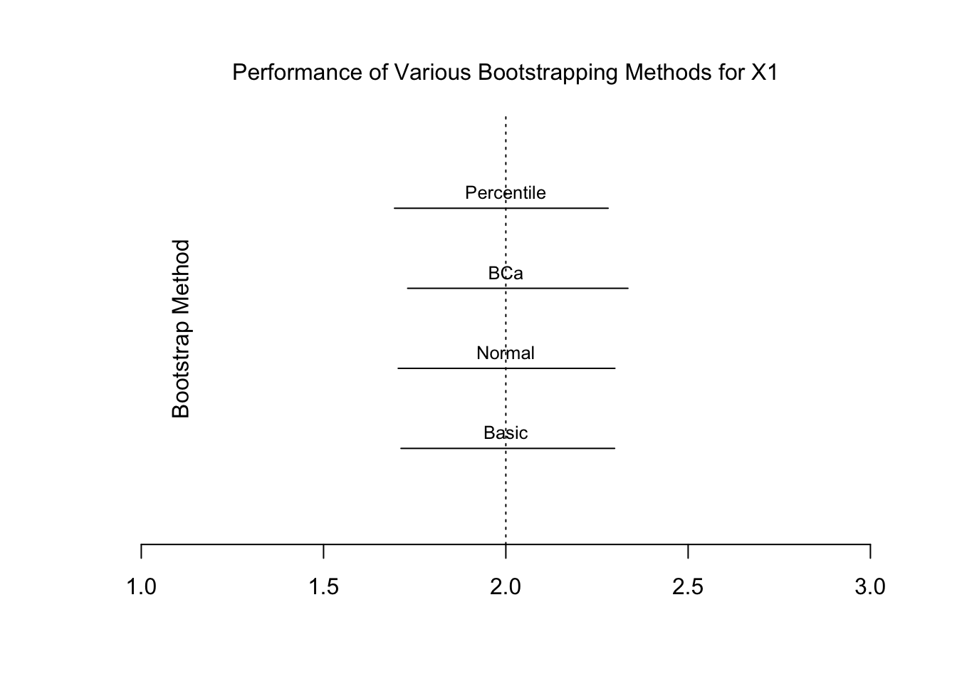
Para \(X_2\)
## BOOTSTRAP CONFIDENCE INTERVAL CALCULATIONS
## Based on 1000 bootstrap replicates
##
## CALL :
## boot.ci(boot.out = bs.res, type = "basic", index = 3)
##
## Intervals :
## Level      Basic
## 95%   (-5.101, -4.588 )
## Calculations and Intervals on Original Scaleplot(NULL, type = "l", xlim = c(-6,-4),ylim = c(0,5), ylab = NA, axes = FALSE, xlab = NA)
lines(c(bs.basic.x2$basic[4], bs.basic.x2$basic[5]), c(1,1)) # add the 95% confidence intervals
text(-5, 1.2, "Basic", xpd = T, cex = .8) # add the names
lines(c(bs.norm.x2$norm[2], bs.norm.x2$norm[3]), c(2,2))
text(-5, 2.2, "Normal", xpd = T, cex = .8)
lines(c(bs.bca.x2$bca[4], bs.bca.x2$bca[5]), c(3,3))
text(-5, 3.2, "BCa", xpd = T, cex = .8)
lines(c(bs.perc.x2$perc[4], bs.perc.x2$perc[5]), c(4,4))
text(-5, 4.2, "Percentile", xpd = T, cex = .8)
abline(v = -5.0, lty = 3, col = "black") # añada vertial
axis(side = 1) # add x axis
mtext(side = 2, "Bootstrap Method", line = -3) # tamaño de etiqueta
mtext(side = 3, "Performance de varios métodos por X2", line = 1) # add a title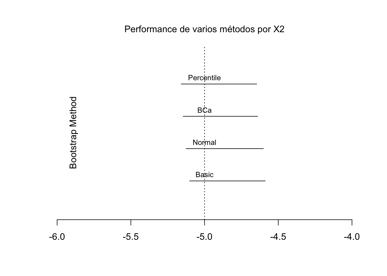
Al menos en este ejemplo, los intervalos de confianza parecen ser muy similares en el tipo de método BOOT.
B.2 Jacknife
Jackknifing puede ser útil para analizar si las observaciones influyentes están afectando nuestras estimaciones. Funciona mediante el uso de un proceso de iteración dejar-uno-fuera. Primera carga en la librería bootstrap:
Para usar la función jackknife, necesitamos tener un vector que seleccionemos de los datos, así como también alguna función “theta” a la que especificamos a la que llama esta función.
Para mostrar esto el cuchillo de caza en acción, vamos a reemplazar una observación con un valor atípico grande:
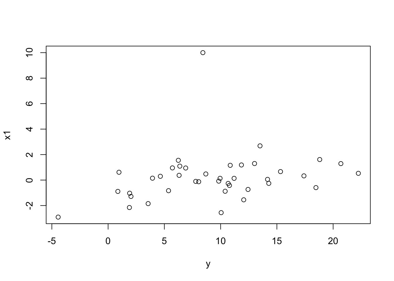
Tenga en cuenta la forma atípica en la parte superior de la distribución.
##
## Call:
## lm(formula = y ~ x1 + x2)
##
## Residuals:
##     Min      1Q  Median      3Q     Max
## -6.6224 -0.9929 -0.0083  1.2703  5.1754
##
## Coefficients:
##             Estimate Std. Error t value Pr(>|t|)
## (Intercept)   9.8528     0.3364  29.287  < 2e-16 ***
## x1            0.7877     0.1697   4.642 4.23e-05 ***
## x2           -4.9889     0.3171 -15.734  < 2e-16 ***
## ---
## Signif. codes:  0 '***' 0.001 '**' 0.01 '*' 0.05 '.' 0.1 ' ' 1
##
## Residual standard error: 2.096 on 37 degrees of freedom
## Multiple R-squared:  0.8779, Adjusted R-squared:  0.8713
## F-statistic:   133 on 2 and 37 DF,  p-value: < 2.2e-16
Observe cuánto ha cambiado nuestra estimación del coeficiente (era \(\sim\) 2, ahora \(\sim\) 0.8). Así que es bastante claro que este extremo atípico está alterando drásticamente nuestros resultados.
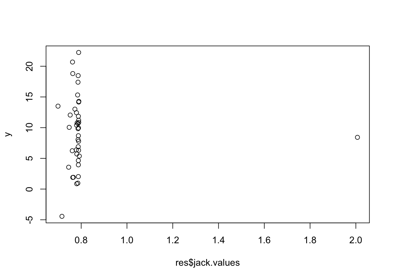
Para Jackknife, primero creamos la función theta. especificamos los datos, el coeficiente y el coeficiente de no entrada, que nos gustaría
Luego ejecuta el jackknife, usando el programa theta, para obtener el \(x_1\) coef.
library(bootstrap)
res <- jackknife(1:length(x1), theta, dat = my.data, coefficient = "x1")

print(res)
## $jack.se
## [1] 1.206817
##
## $jack.bias
## x1
## 0.7376129
##
## $jack.values
## [1] 0.7476185 0.7887048 0.7889221 0.7875193 0.7452521 0.7860689 0.7876873
## [8] 0.7621247 0.7890683 2.0069654 0.7885327 0.7860024 0.7725170 0.7877010
## [15] 0.7804501 0.7843675 0.7876708 0.7870409 0.6987357 0.7875269 0.7632969
## [22] 0.7881386 0.7792951 0.7868219 0.7655709 0.7853704 0.7519223 0.7823062
## [29] 0.7888674 0.7862499 0.7917846 0.7609885 0.7797582 0.7892338 0.7785516
## [36] 0.7631919 0.7808075 0.7158900 0.7896992 0.7862236
##
## $call
## jackknife(x = 1:length(x1), theta = theta, dat = my.data, coefficient = "x1")Si llamamos res, obtenemos una salida del jackknifed, es decir, el sesgo, así como los valores para cada observación individual:
## $jack.se
## [1] 1.206817
##
## $jack.bias
##        x1
## 0.7376129
##
## $jack.values
##  [1] 0.7476185 0.7887048 0.7889221 0.7875193 0.7452521 0.7860689 0.7876873
##  [8] 0.7621247 0.7890683 2.0069654 0.7885327 0.7860024 0.7725170 0.7877010
## [15] 0.7804501 0.7843675 0.7876708 0.7870409 0.6987357 0.7875269 0.7632969
## [22] 0.7881386 0.7792951 0.7868219 0.7655709 0.7853704 0.7519223 0.7823062
## [29] 0.7888674 0.7862499 0.7917846 0.7609885 0.7797582 0.7892338 0.7785516
## [36] 0.7631919 0.7808075 0.7158900 0.7896992 0.7862236
##
## $call
## jackknife(x = 1:length(x1), theta = theta, dat = my.data, coefficient = "x1")Note la observación en 10. Esto es más fácil si lo graficamos:
Aunque Jackknife podría considerarse más intuitivo, es un método más antiguo, más fácil (en el poder de la computación) que abarca el arranque. Probablemente se debe usar el programa de arranque, aunque Jackknife es bueno para examinar esos valores atípicos.