13 Bosques Aleatorios (Random Forest)

Librerías usadas en esta sección

tree

uu <- "https://raw.githubusercontent.com/vmoprojs/DataLectures/master/challengePredTrain.xlsx"
datos <- rio::import(uu)

Primero usamos árboles de clasificación para analizar el conjunto de datos de “Clientes” (https://github.com/vmoprojs/DataLectures/blob/master/challengePredTrain.xlsx).

En estos datos, “Ingresos” es una variable continua, por lo que comenzamos recodificándola como una variable de tres clases Usamos la función ifelse () para crear una variable, llamada IngCat:

A: [0,1500)
B: [1500,2500)
C: >=2500.

library(ISLR2)
datos$IngCat <- with(datos,factor(ifelse(Ingreso <2500, "A","B")))

# Eliminamos/codificamos variables que no aportan
datos$Ingreso <- NULL
datos$No. <- NULL
datos$DPTO_Domicilio <- with(datos,factor(ifelse(DPTO_Domicilio=="LIMA","Capital","Otro")))
datos$Sexo <- factor(datos$Sexo)
datos$IndicadorLaboral <- factor(datos$IndicadorLaboral)

Aquí aplicamos el bagging y los bosques aleatorios a los datos de Clientes, usando el paqueterandomForest en R.

Los resultados exactos obtenidos en esta sección pueden depender de la versión de R y la versión del paquete randomForest instalado en su computadora.

La función randomForest () se puede usar para realizar tanto bosques aleatorios como bagging.

Realizamos el bagging de la siguiente manera:

set.seed(8519)
train <- sample(1:nrow(datos), nrow(datos)*.7)
library(randomForest)

## randomForest 4.7-1.1

## Type rfNews() to see new features/changes/bug fixes.

## 
## Attaching package: 'randomForest'

## The following object is masked from 'package:psych':
## 
##     outlier

## The following object is masked from 'package:ggplot2':
## 
##     margin

## The following object is masked from 'package:dplyr':
## 
##     combine

set.seed(1)
bag.ing <- randomForest(IngCat ~ ., data = datos,
    subset = train, mtry = 16, importance = TRUE,ntree = 500)
bag.ing

## 
## Call:
##  randomForest(formula = IngCat ~ ., data = datos, mtry = 16, importance = TRUE,      ntree = 500, subset = train) 
##                Type of random forest: classification
##                      Number of trees: 500
## No. of variables tried at each split: 16
## 
##         OOB estimate of  error rate: 33.15%
## Confusion matrix:
##      A   B class.error
## A 1021 314   0.2352060
## B  427 473   0.4744444

El argumento mtry = 12 indica que \(12\) predictores deben ser considerados para cada división del árbol, en otras palabras, que el bagging debe hacerse.

¿Qué tan bien funciona este modelo en datos de prueba?

y.test <- datos[-train, "IngCat"]
yhat.bag <- predict(bag.ing, newdata = datos[-train, ])
tt <- table(yhat.bag,y.test)
sum(diag(tt))/sum(tt)

## [1] 0.6673618

Tenemos que el accuracy es 50.8%

Ahora hacemos la predicción usando la variable dependiente cuantitativa:

uu <- "https://raw.githubusercontent.com/vmoprojs/DataLectures/master/challengePredTrain.xlsx"
datos <- rio::import(uu)
# Eliminamos/codificamos variables que no aportan
datos$No. <- NULL
datos$DPTO_Domicilio <- with(datos,factor(ifelse(DPTO_Domicilio=="LIMA","Capital","Otro")))
datos$Sexo <- factor(datos$Sexo)
datos$IndicadorLaboral <- factor(datos$IndicadorLaboral)

set.seed(8519)
train <- sample(1:nrow(datos), nrow(datos)*.7)
library(randomForest)
set.seed(1)
bag.ing2 <- randomForest(Ingreso ~ ., data = datos,
    subset = train, mtry = 16, importance = TRUE,ntree = 500)
bag.ing2

## 
## Call:
##  randomForest(formula = Ingreso ~ ., data = datos, mtry = 16,      importance = TRUE, ntree = 500, subset = train) 
##                Type of random forest: regression
##                      Number of trees: 500
## No. of variables tried at each split: 16
## 
##           Mean of squared residuals: 3804772
##                     % Var explained: 10.75

y.test <- datos[-train, "Ingreso"]
yhat.rf <- predict(bag.ing2, newdata = datos[-train, ])
mean((yhat.rf - y.test)^2)

## [1] 4823805

set.seed(8519)
train <- sample(1:nrow(datos), nrow(datos)*.7)
library(randomForest)
set.seed(1)
bag.ing3 <- randomForest(Ingreso ~ ., data = datos,
    subset = train, mtry = 8, importance = TRUE,ntree = 500)
bag.ing3

## 
## Call:
##  randomForest(formula = Ingreso ~ ., data = datos, mtry = 8, importance = TRUE,      ntree = 500, subset = train) 
##                Type of random forest: regression
##                      Number of trees: 500
## No. of variables tried at each split: 8
## 
##           Mean of squared residuals: 3730752
##                     % Var explained: 12.48

yhat.rf3 <- predict(bag.ing3, newdata = datos[-train, ])
mean((yhat.rf3 - y.test)^2)

## [1] 4505711

Ahora veamos gráficamente. Los resultados indican que en todos los árboles considerados en el bosque aleatorio, IndicadorLaboral y Saldo_Total_Comp_SinHip_C son las dos variables más importantes.

importance(bag.ing3)

##                                %IncMSE IncNodePurity
## Sexo                         7.7390385     177972396
## IndicadorLaboral            26.4856834     823583236
## FlagVehicular               -0.5151038      78540698
## EdadAnio                     1.3509589     594117844
## DPTO_Domicilio               1.2456624      61418531
## Num_Ent_CompSinH_C          12.0003443     306738740
## TieneTarjeta_Comp_C          4.6960956      51144755
## Saldo_TarjetaComp_C         13.5075050     903067978
## Saldo_Total_Comp_SinHip_C   17.7982802    1079660371
## VarMax_3_4a18M              10.7103140     751447364
## PeorCalif_U36M               2.6849525     180907906
## PeorCalif_U12M               0.1679927      56564381
## Bancarizacion_U36M          20.1688891     796569425
## Bancarizacion_U12M          14.0737052     266188070
## PromeSaldoCompSinHip_U4_18M 16.6296639    1083799647
## MaxSaldoCompSinHip_U4_18M   20.6947613    1475993419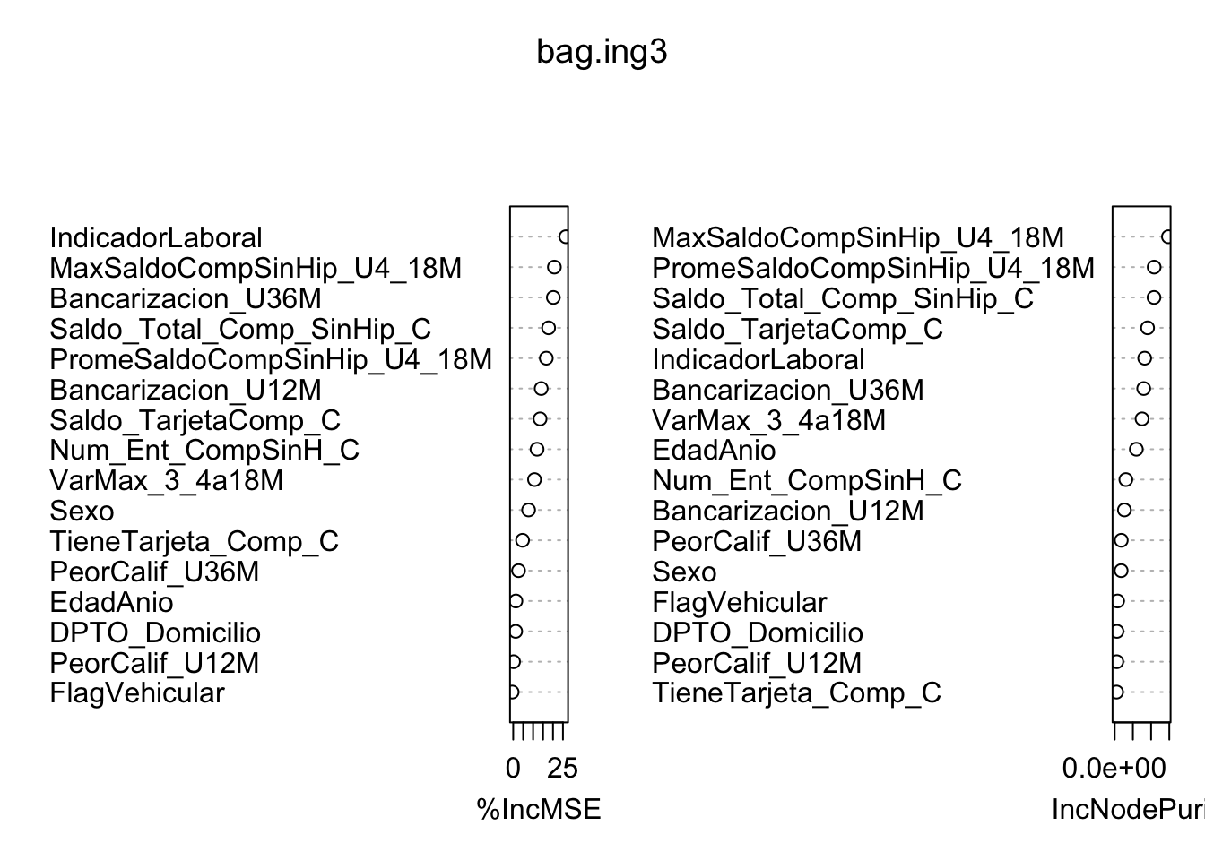

varImpPlot(bag.ing3)

Volvamos a los datos categorizamos y calculamos el accuracy:

yhat.cat <- factor(ifelse(yhat.rf3 <2500, "A","B"))
y.test.cat <- factor(ifelse(y.test <2500, "A","B"))
tt1 <- table(yhat.cat,y.test.cat)
sum(diag(tt1))/sum(tt1)

## [1] 0.6684046

En este caso, el recategorizar resulta perjudicial.

13.1 Usando caret

Diseñamos una estructura que busca el número de covariables a incluir. Usamos una validación cruzada en 5 grupos con 2 repeticiones.

library(caret)
control <- trainControl(method='repeatedcv', 
                        number=3, 
                        repeats=1, 
                        search='grid')
tunegrid <- expand.grid(.mtry = (13:14)) 

rf_gridsearch <- caret::train(Ingreso ~ ., 
                       data = datos[-train, ],
                       method = 'rf',
                       metric = 'RMSE',ntree = 50,
                       tuneGrid = tunegrid)
print(rf_gridsearch)

## Random Forest 
## 
## 959 samples
##  16 predictor
## 
## No pre-processing
## Resampling: Bootstrapped (25 reps) 
## Summary of sample sizes: 959, 959, 959, 959, 959, 959, ... 
## Resampling results across tuning parameters:
## 
##   mtry  RMSE      Rsquared    MAE     
##   13    2060.000  0.06279440  1159.403
##   14    2077.995  0.06314295  1166.208
## 
## RMSE was used to select the optimal model using the smallest value.
## The final value used for the model was mtry = 13.

Ahora iteramos sobre una lista para estimar el número de árboles:

modellist <- list()

for (ntree in c(50,100))
{
  set.seed(123)
  fit <- caret::train(Ingreso ~ ., 
                       data = datos[-train, ],
                       method = 'rf',
                       metric = 'RMSE',ntree = ntree,
                       tuneGrid = tunegrid)
  key <- toString(ntree)
  cat("Numero de arboles: ",ntree,"\n")
  modellist[[key]] <- fit
}

#Comparando resultados
results <- resamples(modellist)
summary(results)

dotplot(results)

library(doParallel)
cl <- makePSOCKcluster(5)
registerDoParallel(cl)

control <- trainControl(method='repeatedcv', 
                        number=3, 
                        repeats=2, 
                        search='grid')
tunegrid <- expand.grid(.mtry = (5:14)) 

modellist <- list()

for (ntree in c(200,300,500,1000))
{
  set.seed(123)
  fit <- caret::train(Ingreso ~ ., 
                       data = datos[-train, ],
                       method = 'rf',
                       metric = 'RMSE',ntree = ntree,
                       tuneGrid = tunegrid)
  key <- toString(ntree)
  # cat("\n","Numero de arboles: ",ntree,"\n")
  modellist[[key]] <- fit
}

stopCluster(cl)

results <- resamples(modellist)
summary(results)
dotplot(results)

13.1.1 Ejercicio

Comentar detalladamente el siguiente código:

dummies <- dummyVars(~ ., data=datos[,-17])
c2 <- predict(dummies, datos[,-17])
d_d <- as.data.frame(cbind(datos$Ingreso, c2))
names(d_d)[1] <- "Ingreso"

denormalize <- function(x_norm,x_orig)
{
  #x_norm: normalized dats
  #x_orig: original data
  mmin <- min(x_orig);mmax <- max(x_orig)
  denorm_val <- x_norm*(mmax-mmin)+mmin
  return(denorm_val)
}
normalize <- function(x) {
return((x - min(x)) / (max(x) - min(x)))
}
dat_rf <- normalize(d_d)

set.seed(8519)
train <- sample(1:nrow(datos), nrow(datos)*.7)
table(1:nrow(datos)%in%train)

## 
## FALSE  TRUE 
##   959  2235

y.test <- dat_rf[-train, "Ingreso"]
library(randomForest)
set.seed(1)
bag.ing3 <- randomForest(Ingreso ~ ., data = dat_rf,
    subset = train, mtry = 4, importance = TRUE,ntree = 500)
bag.ing3

## 
## Call:
##  randomForest(formula = Ingreso ~ ., data = dat_rf, mtry = 4,      importance = TRUE, ntree = 500, subset = train) 
##                Type of random forest: regression
##                      Number of trees: 500
## No. of variables tried at each split: 4
## 
##           Mean of squared residuals: 0.0001614514
##                     % Var explained: 15.35

yhat.rf3 <- predict(bag.ing3, newdata = dat_rf[-train, ])
mean((yhat.rf3 - y.test)^2)

## [1] 0.000188713

yhat.rf3_orig <- denormalize(yhat.rf3,datos[-train,"Ingreso"])
yhat.test_orig <- denormalize(y.test,datos[-train,"Ingreso"])


yhat.cat <- factor(ifelse(yhat.rf3_orig <2500, "A", "B"))
y.test.cat <- factor(ifelse(yhat.test_orig <2500, "A","B"))
tt2 <- table(yhat.cat,y.test.cat)
tt2

##         y.test.cat
## yhat.cat   A   B
##        A 952   6
##        B   1   0

sum(diag(tt2))/sum(tt2)

## [1] 0.9927007