| Bag | Store | Weight |
|---|---|---|
| 1 | Wilsons | 201.0672 |
| 2 | Wilsons | 191.6699 |
| 3 | Myles | 194.5842 |
| 4 | Myles | 191.2856 |
| 5 | Colemans | 189.9170 |
| 6 | Colemans | 194.9869 |
8 z-test
This chapter will cover a brief example of a z-test. In addition, the concepts of standard error, as relevant for inferential statistics will be explored.
8.1 Betcha’ can’t eat just one!
Imagine we wanted to model the average weight of a bag of Lays Potato Chips. Let’s use our scientific method, as discussed in an ealier chapter, to conduct some science.
Specifically, you have a theory that, despite being listed as 200g, the large bag of chips actually weighs less because the company cuts corners to save money and is, thus, dishonest about the weight. So you hypothesize that Lays chips that are listed as 200g do not weigh 200g.
Step 1: State your hypotheses:
\(H_0: \mu_{lays}=200g\)
\(H_1: \mu_{lays}<200g\)
You email Lays and they say that their chips, on average, weight 200g, but have some variability. Specifically, they say the standard deviation of the chips is 6g. You aren’t satisfied with that response and continue with your research.
Step 2: Criteria and analytic plan
It is impossible for you to weigh every produced ‘200g’ bag of Lays chips, so you decide to take a sample. You decide to use NHST to test the weights of bags and use a \(\alpha=.05\) critereon.
Step 3: Collect your data
You drive around Corner Brook to Mr. Wilson’s, Myle’s, and Colemans, and buy two 200g bags of Lays at each location (n = 6). You get the following data:
Let’s calculate the mean and standard deviation of our bag of chips.
      Mean       SD
1 193.9185 4.017174
8.1.1 Mean, Standard Deviation, and Variance
Remember, the mean is a measure of central tendency and is (here, population):
\(\mu = \frac{\sum_{i=1}^{n} x_{i}}{n}\)
and population standard deviation is:
\(\sigma = \sqrt{\frac{\sum_{i=1}^N (x_i - \overline{x})^2}{N}}\)
and population variance is:
\(\sigma^2 = \frac{\sum_{i=1}^N (x_i - \overline{x})^2}{N}\)
You may remember that the population and sample standard deviation differ in the denominator. The sample SD and variance have \(n-1\) as a denominator versus the population’s \(n\). Why?
Standard deviations are typically biased downward (they underestimate the true standard deviation), so the \(n-1\) makes is less biased. Let’s take an example. Consider a population with a mean of 100 and standard deviation of 15.
Let’s take a sample of 30 people from that population and calculate the standard deviation. We get the following SD:
[1] 11.91149So, because it’s an estimate, it has some degree of error. It’s not expected to be exactly 15. But what it we took 5000 samples?
After I simulated 5,000 sample, I get the following distribution of SD.
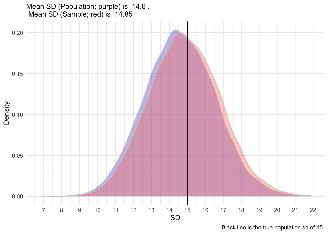
So, as you can see, the sample formula provides a less biased estimate of the true population SD. It’s shifted slightly to the right, closer to the true population SD. We hope that the mean and standard deviation that we collect in a sample (termed statistics) are somewhat good indicators of those in the population (termed parameters).
Practice Question
Calculate the mean, sample SD, and sample variance of the following two variables, x and y:
| x | y |
|---|---|
| 6 | 10 |
| 3 | 6 |
| 12 | 8 |
| 3 | 9 |
| 6 | 4 |
Click for answers.
  Mean_x     SD_x Mean_y     SD_y
1      6 3.674235    7.4 2.408319
8.1.2 Visualizing Chips
Given that Lays has communicated the population parameters, we can calculate how likely our sample is. First, let’s visualize the distribution of chips with a \(\mu=200\) and \(\sigma=6\):
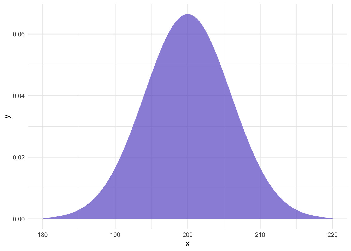
Imagine that the six bags of chips that we sampled somehow came from this distribution. Although most are around 200g, some are much higher or lower. Now, to take it one step further, let’s plot the distribution of sample means. That is, imagine we took a sample of six bags from the above distribution of chips over, and over, and over, and over…
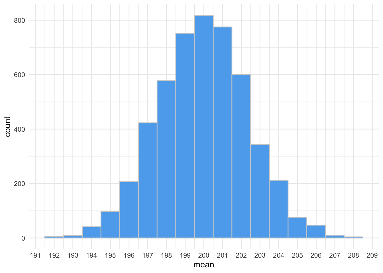
As you can see from the figure, when you collect the mean of six random bags of chips many times, they form another normal distribution. This is known as the distribution of sample means. Central limit theorem (CLT) states that this distribution approximates a normal curve with a mean equal to the population mean and a standard deviation equal to the population standard deviation divided by the square root of the sample size (the standard error).
According to CLT, the mean of the distribution of sample means is:
\(\mu_{\bar{x}} = \mu\)
and the standard error of the means is;
\(\sigma_{\bar{x}} = \frac{\sigma}{\sqrt{n}}\)
Standard Error
The standard error is the standard deviation of sample means. A large standard error indicates high variability between the means of different samples. Therefore, your sample may not be a good representation of the true population mean. This is not good.
A small standard error indicates low variability between the means of different samples. Therefore, our sample mean is likely reflective of the population mean. This is good.
Step 4: Analyse
8.2 z-test
Should the above distribution of sample means truly follow a normal distribution, then we should be able to calculate how likely our sample of six bag of chips is! We can fill in the what we know, according to Lays: \(\mu_{\bar{x}} = \mu = 200\) and; \(\sigma_{\bar{x}} = \frac{\sigma}{\sqrt{n}} = \frac{6}{\sqrt{6}} = 2.4495\)
So, the probability of getting our sample mean of 193.92 can be converted into a z-score: \(z = \frac{x - \bar{x}}{\sigma_{\bar{x}}} = \frac{193.9185 - 200}{2.4495} = -2.482752\)
and the probability of getting a z-score that low is 0.0065. Recall that the normal distribution has some unique properties and we can find out the proportion of scores that fall in the tails. While you may have used table like the previous link in past courses, computers can easily determine the exact quantity (e.g., pnorm() in R). Such that:
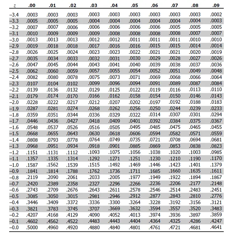
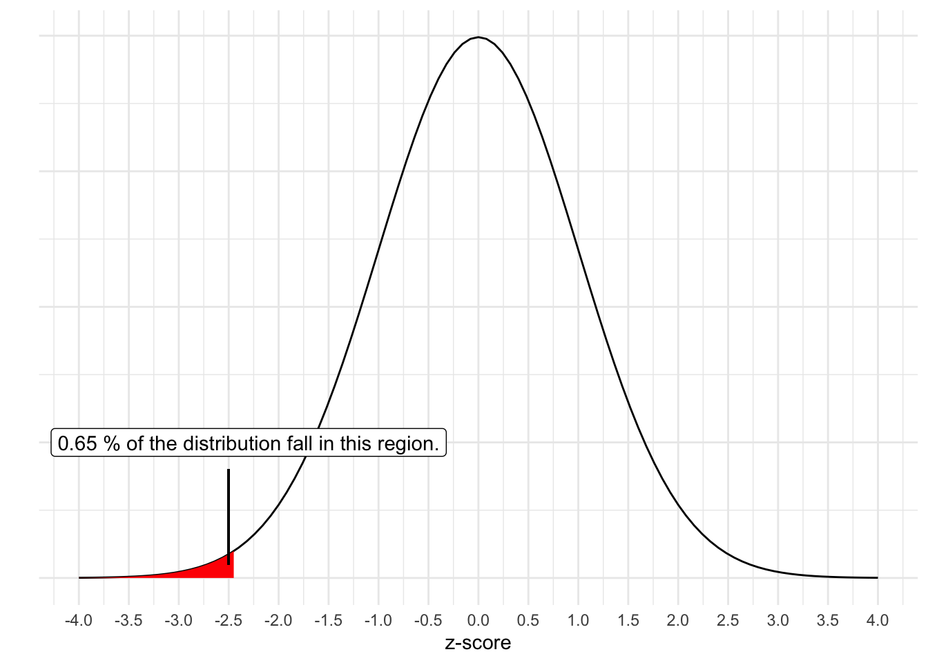
It falls at the 0.65th percentile. So out of 1000 samples of six bags of chips drawn from the distribution of mean 200 and SD of 6, we would get a score this low or lower less than 7 times. Our sample is very unlikely if Lays is telling the truth!
You just did a z-test. Let’s run it in R to ensure we get the same numbers! Recall our data:
| Bag | Store | Weight |
|---|---|---|
| 1 | Wilsons | 201.0672 |
| 2 | Wilsons | 191.6699 |
| 3 | Myles | 194.5842 |
| 4 | Myles | 191.2856 |
| 5 | Colemans | 189.9170 |
| 6 | Colemans | 194.9869 |
The assumption is that we have randomly sampled. That is:
\(H_{0}: \mu = 200\);
and
\(H_{1}: \mu < 200\).
What would you conclude?
    One-sample z-Test

data:  chip_data$Weight
z = -2.4828, p-value = 0.006518
alternative hypothesis: true mean is less than 200
95 percent confidence interval:
       NA 197.9475
sample estimates:
mean of x
 193.9185
Step 5: Write up your results/conclusions
When interpreting this, we can say that the likelihood of getting our sample mean of 193.91 or lower is unlikely given a true null hypothesis that \(\mu=200\), z = -2.48, p = .0065. This is referred to as statistical significance (see later chapter), but in short, our p-value is the probability of obtaining our data or more extreme given a null hypothesis,
\(p(data|hypothesis)\).
Practice Question
What’s the difference is the probability of sampling a single bag of chips weighting 190g in a sample versus getting a mean weight of 190g for 10 bags of chips? Why are they different? How to the distributions differ?
Practice Question
What happens to the SD of the distribution of sample means as the sample size increases? Imagine drawing 100,000 bags of chips.