11 Factorial ANOVA
In progress. Check back soon.
11.1 Our Data
You are hired by the regional health authority to conduct research regarding patient-provider satisfaction. You theorize that female physicians are more compassionate and that patients will rate visits with female physicians higher than male physicians. Furthermore, theory suggests that men are more comfortable around female physicians than male physicians and will, thus, rate these visits as more satisfactory. You recruit 40 individuals (20 men and 20 women) in Corner Brook and ask them to complete a short survey at the end of their next medical appointment. Specifically, you ask them the gender of their health care provider and a short questionnaire on their satisfaction with the appointment (scores range from 1-40). Thus, we have two independent variables (IVs) - patient gender and provider gender - and one dependent variable (DV) - satisfaction. Specifically, you hypothesize that:
- Participants will be more satisfied with visits from female physicians compared to male physicians.
- There will be an interaction between patient and provider gender, such male patients will rate females physicians higher than male physicians, but female patients will not have such a pattern.
You obtain the following data:
| ID | Patient | Provider | Satisfaction |
|---|---|---|---|
| 1 | Male | Male | 21 |
| 2 | Male | Male | 18 |
| 3 | Male | Male | 20 |
| 4 | Male | Male | 19 |
| 5 | Male | Male | 23 |
| 6 | Male | Female | 29 |
| 7 | Male | Female | 29 |
| 8 | Male | Female | 30 |
| 9 | Male | Female | 27 |
| 10 | Male | Female | 29 |
| 11 | Female | Male | 25 |
| 12 | Female | Male | 26 |
| 13 | Female | Male | 28 |
| 14 | Female | Male | 25 |
| 15 | Female | Male | 22 |
| 16 | Female | Female | 22 |
| 17 | Female | Female | 26 |
| 18 | Female | Female | 25 |
| 19 | Female | Female | 18 |
| 20 | Female | Female | 19 |
In the last chapter, we investigated the efficacy of four treatment for obsessive compulsive disorder. In that example, each individual could only be in one group (i.e., someone received CBT or Rx). In the example we just introduced regarding visit satisfaction, we have two independent variables. That is, an individual has a value on both patient and provider gender. To account for this new model, we must extend our knowledge of the one factor ANOVA into a factorial ANOVA.
Factorial ANOVAs have multiple independent variables. These can be between or within (repeated measures) individuals.
11.2 Our Model
We extend the GLM to represent how we will analyse the data. Recall that the basic structure is:
\(outcome_i=model+error_i\)
And our current model will be:
\(y_i=\beta_0+x_{1i}\beta_1+x_{1i}\beta_2+x_{1i}x_{2i}\beta_3+e_i\)
Where \(y_i\) is the satisfaction (DV) score for individual \(i\), \(x_{1i}\) is the gender of individual \(i\), \(x_{2i}\) is the gender of the provider that individual \(i\) visited, and the \(\beta\)s are the associated coefficients. Note that \(x_{1i}x_{2i}\) is simply the individual scores multiplied together. If you recall dummy coding, we would have \(k-1\) variables for each level of a factor. Each of our two IVs have two levels, so they each require one variable to represent them. The resulting summary table may be helpful:
| Patient Gender | Provider Gender | Mean | SD | x1 (Patient Gender Dummy Coded) | x2 (Provider Gender Dummy Coded) | x1 * x2 |
|---|---|---|---|---|---|---|
| Female | Female | 22.0 | 3.54 | 0 | 0 | 0 |
| Female | Male | 25.2 | 2.17 | 0 | 1 | 0 |
| Male | Female | 28.8 | 1.10 | 1 | 0 | 0 |
| Male | Male | 20.2 | 1.92 | 1 | 1 | 1 |
If you recall from the last chapter, we can determine what each coefficient would be. Using the equation and the table, let’s figure out each coefficient would be. First, for female patients and female providers:
\(y_i=\beta_0+x_{1i}\beta_1+x_{1i}\beta_2+x_{1i}x_{2i}\beta_3+e_i\)
Recall that the above represents the equation for each individual, which is why it includes error. However, for a group:
\(FF=\beta_0+(0)\beta_1+(0)\beta_2+(0)(0)\beta_3 = \beta_0\)
Since we know the mean of the female (patient) -female (provider) group is 29.00, we know that \(\beta_0=22.00\). Second, we can solve the equation for female patients (\(x_1=0\)) with male providers (\(x_2=1\)).
\(FM=\beta_0+(0)\beta_1+(1)\beta_2+(0)(1)\beta_3 = \beta_0+\beta_2\)
Since \(\beta_0=22.00\) and the mean of female-patient, male-provider is 25.2, we can determine that:
\(FM= \beta_0+\beta_2\) and
\(\beta_2=25.20-22.00=3.20\)
\(y_i=\beta_0+x_{1i}\beta_1+x_{1i}\beta_2+x_{1i}x_{2i}\beta_3+e_i\)
Before moving, on, try to solve for the other coefficients in the model.
Click to reveal the full equation!
\(y_i=\beta_0+x_{1i}\beta_1+x_{1i}\beta_2+x_{1i}x_{2i}\beta_3+e_i\)
\(y_i=22.00+x_{1i}(6.80)+x_{2i}(3.20)+x_{1i}x_{2i}(-11.80)+e_i\)
11.3 The Interaction
How might you interpret the above? Interactions may seem intimidating, but with some practice you can intuitively understand what they mean. Our interaction term, \(\beta_3=-11.80\), indicates that the relationship between satisfaction and patient/provider differs between men and women. That is, when a female patient rates a male versus female physician, we can expect, on average, a 3.20 increase in satisfaction. This is represented through \(\beta_2=3.20\). However, when a male patient rates a male instead of female physician, we can expect, on average, a 8.60 decrease in satisfaction. This is represented through \(\beta_2+\beta_3=(3.20)+(-11.80)=-8.60\).
Ultimately, an interaction indicates that the relationship between two variables (typically, an IV and DV) depends on a third variable (typically, another IV). One way to help understand and explain interactions is through figures. Consider the following figure.
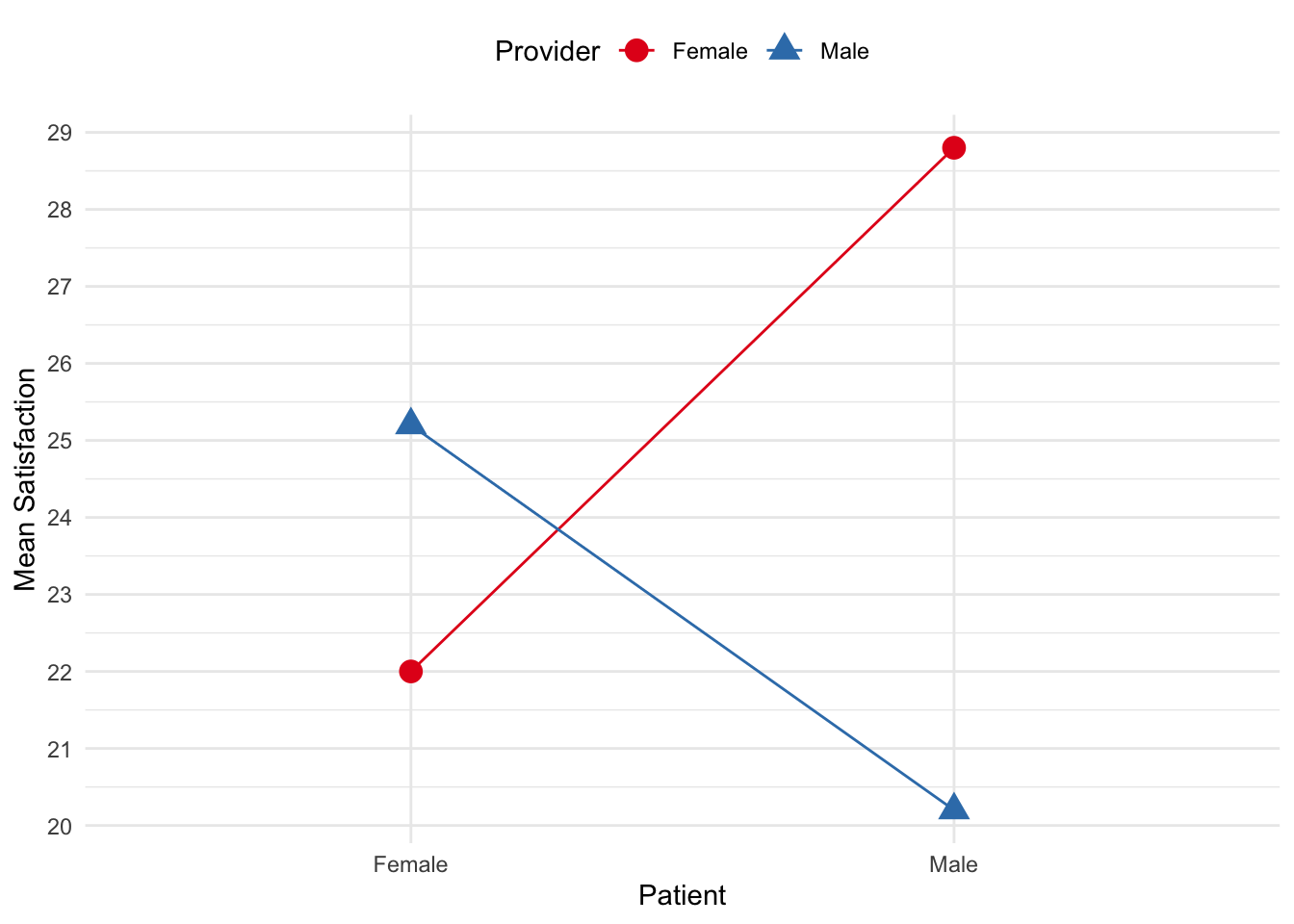
In line with the tip above, the relationship between provider gender and satisfaction differs depending on patient gender. Specifically, female patients reported more satisfaction in appointments with male physicians than female physicians, but the reverse occurred for male patients. Male patients reported more satisfaction with female physicians than male physicians.
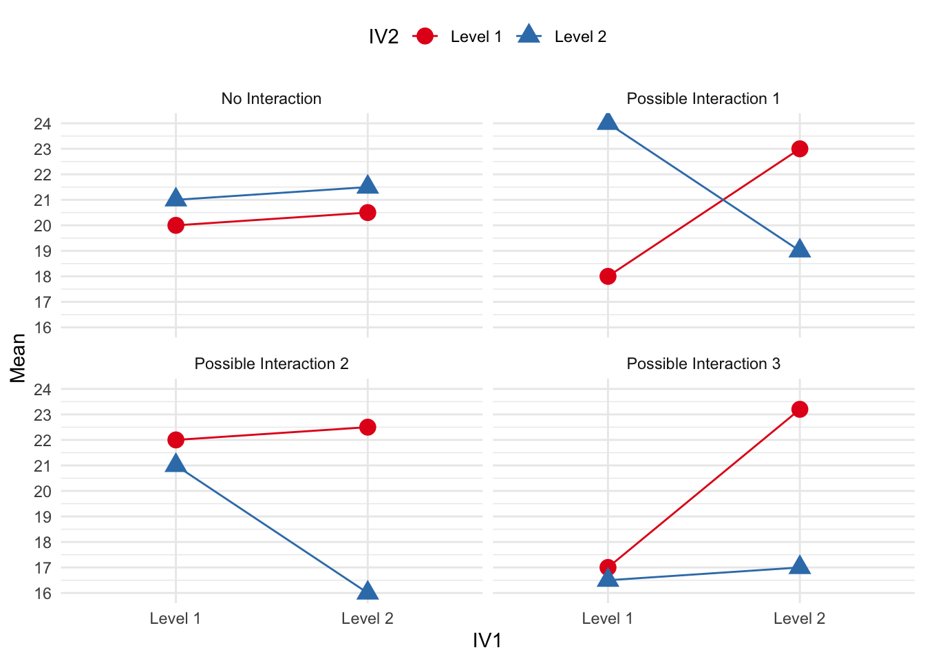
Another way to determine whether an interaction is occurring is to view the slopes of the lines. Parallel lines typically indicate no interaction. As the lines become more perpendicular, an interaction is more evident. For example, consider the following figures and whether an interaction likely exists. Note: these are example, not exhaustive. Also, recall that our IVs are categorical/nominal. Therefore, don’t let the connecting lines give the illusion of a continuous variable.
However, we need to conduct formal tests to determine if these data indicate a relationship between our IVs and DVs.
11.4 Our Analysis
In the last chapter, we partitioned the variances and deviations into some sub-components. Namely, we had:
\(SST = SSB+SSE\)
When we have more than one IV, we need to partition the variances up slightly differently. In the one way ANOVA, we had:
However, in factorial ANOVAs (using the example above), we have:
11.5 SST
Our total sum of squares is no different than a one way ANOVA.
\(SST=\sum_{i=1}^n(x_i-\overline{x}_{grand})^2\) with \(N-1\) degrees of freedom.
For our example, the mean is 24.05. Thus:
\(SST=(21-24.05)^2+(18-24.05)^2...(x_n-24.05)^2=302.95\)
11.6 SSB
We can calculate the total SSB the same way we did for a one factor ANOVA:
\(SSB=\sum_{j=1}^nn_j(\overline{x}_j-\overline{x}_{grand})^2\) with \(k-1\) degrees of freedom.
Although we have two IVs, we want to consider each cell a group. One way to help you visualize this is a table. For our patient-provider example:
| Provider | |||
|---|---|---|---|
| Female | Male | ||
| Patient | Female | \(\overline{x}_1-22.0\) | \(\overline{x}_2=25.2\) |
| Male | \(\overline{x}_3=28.8\) | \(\overline{x}_4=20.2\) |
Thus, we will have four cell to calculate \(SSB\). Recall, our grand mean is 24.05 and the group means are above.
\(SSB=\sum_{j=1}^nn_j(\overline{x}_j-\overline{x}_{grand})^2 = 5(22.0-24.05)^2+5(25.2-24.05)^2+5(28.8-24.05)^2+5(20.2-24.05)^2 = 214.55\)
Now, we will discuss how to break up the SSB into it’s various subcomponents.
11.6.1 IV1
PATIENT GENDER
We can calculate the SS for IV1 the same way we would for a one factor ANOVA. Consider only the patient’s gender. I have collapsed the table from above to account for this.
| Patient | Female | \(\overline{x}_{patientf}=23.60\) |
| Male | \(\overline{x}_{patientm}=24.5\) |
In the last chapter, you learned that we could calculate the SSB by:
\(SSB_{patient}=\sum_{n=1}^jn_j(\overline{x}_j-\overline{x}_{grand})^2\) with \(j-1\) degrees of freedom (i.e., the number of groups in that factor minus 1)
With our data:
\(SSB_{patient}=10(23.60-24.05)^2+10(24.50-24.05)^2=4.05\)
11.6.2 IV2
PROVIDER GENDER We can calculate the SS for IV2 the same way we would for a one factor ANOVA. Consider only the provider’s gender. I have collapsed the original table from above to account for this.
| Provider | ||
|---|---|---|
| Female | Male | |
| \(\overline{x}_{providerf}=25.40\) | \(\overline{x}_{providerm}=22.70\) |
and, thus:
\(SSB_{provider}=\sum_{n=1}^jn_j(\overline{x}_j-\overline{x}_{grand})^2\) with \(j-1\) degrees of freedom (i.e., the number of groups in that factor minus 1)
With our data:
\(SSB_{provider}=10(25.40-24.05)^2+10(22.70-24.05)^2=36.45\)
11.6.3 The Interaction
Now here comes the hard part! Kidding. You know that SSB = sum of all IV components including interactions. We can easily calculate the #SSB_{interaction}$ by subtracting our two main factors from our total SSB.
\(SSB_{interaction}=SSB-SSB_{IV1}-SSB_{IV2}\)
\(SSB_{interaction}=214.55-4.05-36.45=174.05\)
Similarly, the interaction term \(df\) are the \(SSB\) minus main effect \(df\).
\(df_{interaction}=df_{SSB}-df_{IV1}-df_{IV2}\)
here:
\(df_{interaction}=3-1-1=1\)
11.7 SSE
The last thing we need is the SSE for the errors/residuals. You recall that our formula for SSE is:
\(SSE=\sum_{j=1, i=1}^n(x_{ij}-\overline{x}_j)^2\)
A shortcut method may be to use:
\(SSE=\sum_{j=1}^ns_j^2(n_j-1)\) (the sum of the variances multiplied by \(n-1\) for each group).
The variances for each of the groups for us is:
dat_pp %>%
  group_by(Patient, Provider) %>%
  summarise(Variance=var(Satisfaction),
            Size=n()) %>%
  kbl() %>%
  kable_styling(full_width = F)
`summarise()` has grouped output by 'Patient'. You can override using the
`.groups` argument.| Patient | Provider | Variance | Size |
|---|---|---|---|
| Female | Female | 12.5 | 5 |
| Female | Male | 4.7 | 5 |
| Male | Female | 1.2 | 5 |
| Male | Male | 3.7 | 5 |
Therefore, our SSE is:
\(SSE=12.5(4)+4.7(4)+1.2(4)+3.7(4)=88.40\)
11.8 Mean Squares
Our mean squares are calculated the same as before, matching each SS with their respective \(df\).
\(MS_{patient}=\frac{SS_{patient}}{df_{patient}}=\frac{4.095}{1}=4.05\)
\(MS_{provider}=\frac{SS_{provider}}{df_{provider}}=\frac{36.45}{1}=36.45\)
\(MS_{interaction}=\frac{SS_{interaction}}{df_{interaction}}=\frac{174.05}{1}=174.05\)
and for our error:
\(MS_{error}=\frac{SSE}{df_{error}}=\frac{88.40}{16}=5.525\)
11.9 F Statistic
The F statistics will be calculated the same way as a one way ANOVA. However, we will now have three tests: one for each main effect and interaction.
\(F_{patient}=\frac{MS_{patient}}{MSE}=\frac{4.05}{5.525}=0.733\)
\(F_{provider}=\frac{MS_{provider}}{MSE}=\frac{36.45}{5.525}=6.60\)
\(F_{interaction}=\frac{MS_{interaction}}{MSE}=\frac{174.05}{5.525}=31.50\)
The p-value for each statistic can be calculated for each F statistic using an F-Distribution table. Find a table here and a calculator here.
Our p-values are: * Patient - p = .405 * Provider - p = .021 * Interaction - p < .001
11.10 Effect Size
We will use an effect size similar to the one we used for one way ANOVA. However, we will adjust the formula to account for only the ratio of variance explained by a factor relative to the unexplained variance. This effect size is called partial eta squared (\(\eta_p^2\)).
\(\eta_p^2=\frac{SS_{factor}}{SS_{factor}+SSE}\)
For patients:
\(\eta_p^2=\frac{SS_{patient}}{SS_{patient}+SSE}=4.05/(4.05+88.40)=.043\)
Calculate the other \(\eta_p^2\)s!
Click to reveal the other effect sizes!
Providers: \(\eta_p^2=\frac{SS_{provider}}{SS_{provider}+SSE}=36.54/(36.45+88.40)=.293\) Interaction: \(\eta_p^2=\frac{SS_{interaction}}{SS_{interaction}+SSE}=174.05/(174.05+88.40)=.663\)
11.11 Our Post-hoc Analysis
Remember, the omnibus ANOVA tells us that the group differ, but not how. Furthermore, you should always be mindful that main effects may not tell the full story when the interaction is statistically significant. Thus, the interaction should be the main foci of interpretation when it is statistically significant. While there are many ways to conduct post-hoc analyses (e.g., contrast), I would focus on Bonferroni corrected t-test on the a priori analyses of interest.
Specifically, we would conduct individual analyses of one IV –> DV on other the various levels of the other IV. These are called simple effects. For example, we could look at the effect of Provider Gender on Satisfaction separately for female and male patients.
11.12 Our Results
Typically, we would report the following in order:
- Main effect 1
- Main effect 2
- Main effect… \(n\)
- Interactions
- Post-hoc/simple effects
Be sure to address your research questions/hypotheses.
Recall our hypotheses: 1. Participants will be more satisfied with visits from female physicians compared to male physicians. 2. There will be an interaction between patient and provider gender, such male patients will rate females physicians higher than male physicians, but female patients will not have such a pattern.
In detail: 1. Participants will be more satisfied with visits from female physicians compared to male physicians.
The results suggest that our data unlikely given a true null that satisfaction is equal for both male and female providers, F(1, 16) = 6.60, p = .021; \(\eta_p^2\) = .29, 95% CI [0.03, 1.00]. Thus, our hypothesis were supported.
- There will be an interaction between patient and provider gender, such male patients will rate females physicians higher than male physicians, but female patients will not have such a pattern.
The interaction between Patient and Provider is statistically significant and large, F(1, 16) = 31.50, p < .001; \(\eta_p^2\) = 0.66, 95% CI [0.40, 1.00]).
And now, our post-hoc analyses investigating the effect of provider effect on satisfaction for male and female patients.
11.12.0.1 Male Patients
We can conduct a t-test using only the male data. Please see the t-test section for details.
    Welch Two Sample t-test

data:  Satisfaction by Provider
t = 8.6873, df = 6.3477, p-value = 9.401e-05
alternative hypothesis: true difference in means is not equal to 0
95 percent confidence interval:
  6.209479 10.990521
sample estimates:
mean in group Female   mean in group Male
                28.8                 20.2
Effect sizes were labelled following Cohen’s (1988) recommendations.
The Welch Two Sample t-test testing the difference of Satisfaction by Provider (mean in group Female = 28.80, mean in group Male = 20.20) suggests that the effect is positive, statistically significant, and large (difference = 8.60, 95% CI [6.21, 10.99], t(6.35) = 8.69, p < .001; Cohen’s d = 6.90, 95% CI [2.86, 10.88]).
11.12.0.2 Female Patients
    Welch Two Sample t-test

data:  Satisfaction by Provider
t = -1.7253, df = 6.6354, p-value = 0.1305
alternative hypothesis: true difference in means is not equal to 0
95 percent confidence interval:
 -7.635051  1.235051
sample estimates:
mean in group Female   mean in group Male
                22.0                 25.2
Effect sizes were labelled following Cohen’s (1988) recommendations.
The Welch Two Sample t-test testing the difference of Satisfaction by Provider (mean in group Female = 22.00, mean in group Male = 25.20) suggests that the effect is negative, statistically not significant, and large (difference = -3.20, 95% CI [-7.64, 1.24], t(6.64) = -1.73, p = 0.130; Cohen’s d = -1.34, 95% CI [-2.98, 0.38]).
Please note that these results are automated and you must adjust for APA formatting.
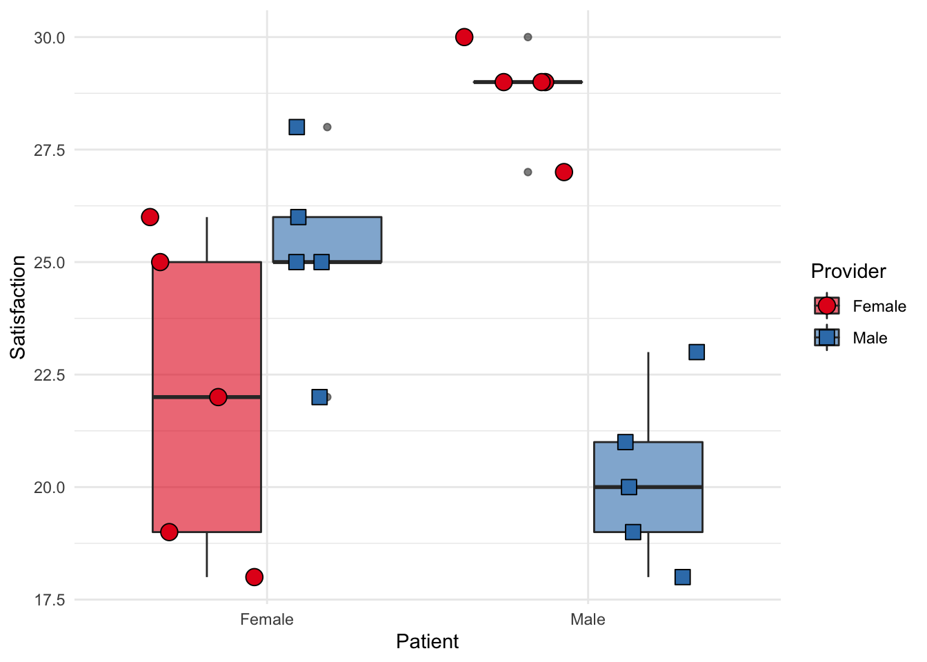
11.13 Visualizing the ANOVA
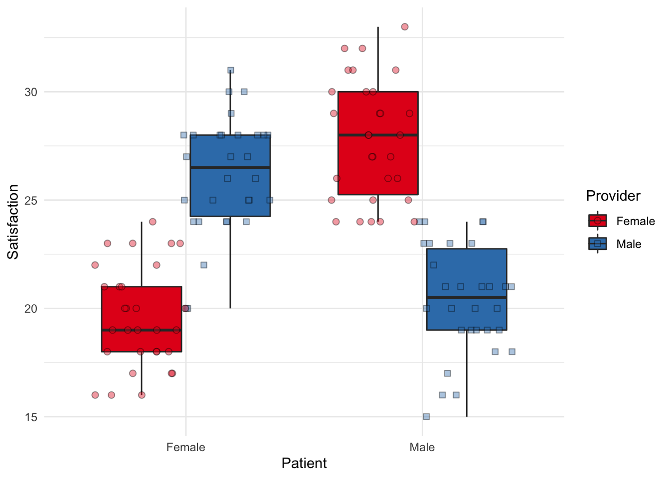
Much like the last chapter, we can visualize the ANOVA using boxplots. Note that we only have five people per cell, so our boxplot is looking bare.
Other times with more participants, it may look more like actual boxes (!). Such as with the following fake data:
Otherwise, we can plot the means and SEs.
pp_sum <- pp_sum %>%
  mutate(n=5) %>%
  mutate(SE=SD/sqrt(n)) %>%
  mutate(ciMult = qt(.95/2 + .5, 5-1)) %>%
  mutate(CI=SE*ciMult)
pd <- position_dodge(0.1)
ggplot(pp_sum, aes(x=Patient, y=Mean, colour=Provider, group=Provider)) +
    geom_errorbar(aes(ymin=Mean-CI, ymax=Mean+CI, colour=Provider), width=.2, position=pd) +
    geom_line(position=pd, aes(colour=Provider)) +
    geom_point(position=pd, size=3, aes(colour=Provider, shape=Provider))+
  scale_color_brewer(palette = "Set1")+
  coord_cartesian(ylim=c(1, 40))+
  scale_y_continuous(breaks = seq(0, 40, 5))+
  theme_minimal()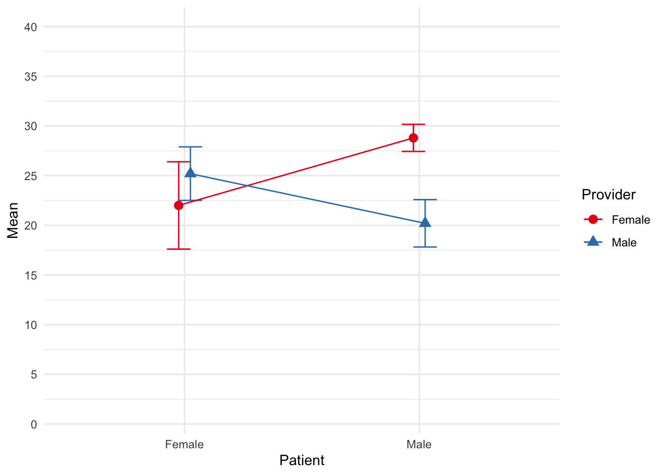
11.14 Factorial ANOVA in R
ANOVAs in R are ‘ez’. The ez library allows for easily running various types of ANOVA, including mixed, factorial, and one way. It also includes relevant assumption tests.
library(ez)
# and the main function
ezANOVA(data = dat_pp, # this is what I named our main data file
        dv = Satisfaction, # specify the dependent variable
        between = c(Provider, Patient), # concatonated list of IVs
        wid = ID) #participant ID
Warning: Converting "ID" to factor for ANOVA.Warning: Converting "Provider" to factor for ANOVA.Warning: Converting "Patient" to factor for ANOVA.Coefficient covariances computed by hccm()$ANOVA
Effect DFn DFd F p p<.05 ges
1 Provider 1 16 6.5972851 2.061606e-02 * 0.29195034
2 Patient 1 16 0.7330317 4.045427e-01 0.04380746
3 Provider:Patient 1 16 31.5022624 3.890118e-05 * 0.66317394
$`Levene's Test for Homogeneity of Variance`
DFn DFd SSn SSd F p p<.05
1 3 16 12.55 28.4 2.356808 0.1102459 11.15 Practice Question
You work with Disney+ and are responsible for researching audience reception for prospective shows. You are testing the effect of having various main characters for a new teen cartoon. Specifically, the show revolves around a superhero and a sidekick. The superhero can be a dog, cat, or rabbit. The sidekick can be a teen boy or girl.
Based on previous shows, you hypothesize that the cat would be more popular than the dog and bird as main characters. Furthermore, you believe a girl sidekick would be more popular than a boy sidekick. However, you think that differences in animal as a main superhero depend on the sidekick. Specifically, there will be no difference in animal popularity when the sidekick is male, but there cats will be more popular than dogs or birds when the sidekick is female.
After showing six difference groups (\(n=5\) for each group) a pilot episode featuring different combination of superheros and sidekicks, you measure their rating of the show (0-100).
You decide to test the data using a 3 (Cat/Dog/Bird) x 2 (Male/Female Sidekick) ANOVA. Your data are as follows:
| ID | Superhero | Sidekick | Rating |
|---|---|---|---|
| 1 | Cat | Male | 52 |
| 2 | Cat | Male | 44 |
| 3 | Cat | Male | 48 |
| 4 | Cat | Male | 48 |
| 5 | Cat | Male | 46 |
| 6 | Dog | Male | 43 |
| 7 | Dog | Male | 49 |
| 8 | Dog | Male | 50 |
| 9 | Dog | Male | 50 |
| 10 | Dog | Male | 48 |
| 11 | Bird | Male | 48 |
| 12 | Bird | Male | 43 |
| 13 | Bird | Male | 44 |
| 14 | Bird | Male | 45 |
| 15 | Bird | Male | 45 |
| 16 | Cat | Female | 69 |
| 17 | Cat | Female | 68 |
| 18 | Cat | Female | 70 |
| 19 | Cat | Female | 73 |
| 20 | Cat | Female | 69 |
| 21 | Dog | Female | 54 |
| 22 | Dog | Female | 63 |
| 23 | Dog | Female | 58 |
| 24 | Dog | Female | 59 |
| 25 | Dog | Female | 59 |
| 26 | Bird | Female | 45 |
| 27 | Bird | Female | 52 |
| 28 | Bird | Female | 47 |
| 29 | Bird | Female | 42 |
| 30 | Bird | Female | 52 |
Click to reveal the answer.
The ANOVA (formula: Rating ~ Superhero + Sidekick + Superhero * Sidekick) suggests that:
- The main effect of Superhero is statistically significant and large (F(2, 24) = 42.87, p < .001; Eta2 (partial) = 0.78, 95% CI [0.63, 1.00])
- The main effect of Sidekick is statistically significant and large (F(1, 24) = 115.82, p < .001; Eta2 (partial) = 0.83, 95% CI [0.71, 1.00])
- The interaction between Superhero and Sidekick is statistically significant and large (F(2, 24) = 26.93, p < .001; Eta2 (partial) = 0.69, 95% CI [0.49, 1.00])
Effect sizes were labelled following Field’s (2013) recommendations.
For female sidekicks:
The ANOVA (formula: Rating ~ Superhero) suggests that:
- The main effect of Superhero is statistically significant and large (F(2, 12) = 55.50, p < .001; Eta2 = 0.90, 95% CI [0.78, 1.00])
Effect sizes were labelled following Field’s (2013) recommendations.
Subsequent ttests:
Cat v Dog
Effect sizes were labelled following Cohen’s (1988) recommendations.
The Welch Two Sample t-test testing the difference between sh_female_cat and sh_female_dog (mean of x = 69.80, mean of y = 58.60) suggests that the effect is positive, statistically significant, and large (difference = 11.20, 95% CI [7.19, 15.21], t(6.55) = 6.69, p < .001; Cohen’s d = 4.23, 95% CI [1.65, 6.76])
Bird v Dog
Effect sizes were labelled following Cohen’s (1988) recommendations.
The Welch Two Sample t-test testing the difference between sh_female_bird and sh_female_dog (mean of x = 47.60, mean of y = 58.60) suggests that the effect is negative, statistically significant, and large (difference = -11.00, 95% CI [-16.70, -5.30], t(7.32) = -4.52, p = 0.002; Cohen’s d = -2.86, 95% CI [-4.72, -0.92])
Cat v Bird
Effect sizes were labelled following Cohen’s (1988) recommendations.
The Welch Two Sample t-test testing the difference between sh_female_cat and sh_female_bird (mean of x = 69.80, mean of y = 47.60) suggests that the effect is positive, statistically significant, and large (difference = 22.20, 95% CI [16.83, 27.57], t(5.48) = 10.35, p < .001; Cohen’s d = 6.55, 95% CI [2.59, 10.49])
For male sidekicks:
The ANOVA (formula: Rating ~ Superhero) suggests that:
- The main effect of Superhero is statistically not significant and large (F(2, 12) = 1.91, p = 0.190; Eta2 = 0.24, 95% CI [0.00, 1.00])
Effect sizes were labelled following Field’s (2013) recommendations.