16 Moderation
In progress. Check back soon.
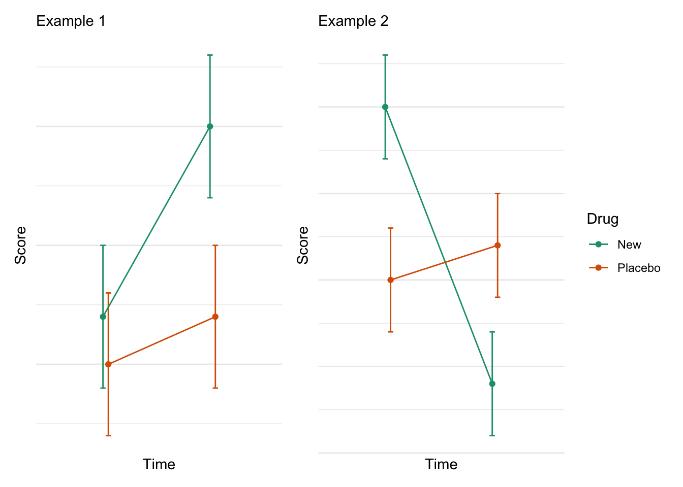
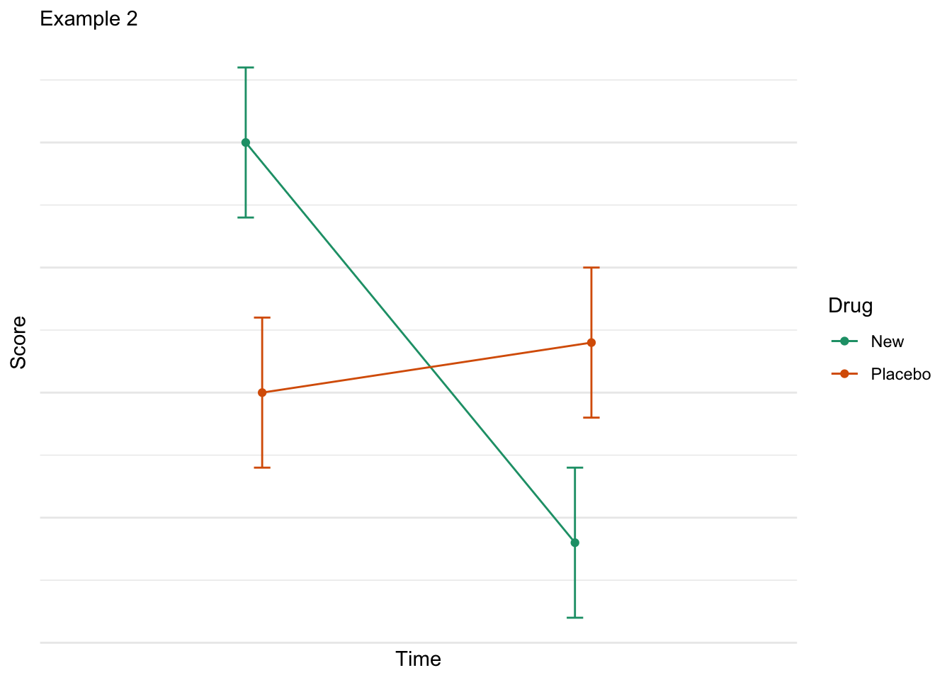
You may not recognize it, but you have much experience with moderation. Quite simply, a moderation is interaction. For example, we may test the efficacy of a new drug versus a placebo on ‘happiness’. We measure scores before taking the drug/placebo, and measure scores after some time of taking the drug/placebo. In this example we have two independent variables (time and drug) and one dependent variable (happiness). An interaction would indicate that the association between an IV and a DV is depenent on some other IV. That is, the change in time on happiness depends on whether you got the drug or the placebo. These figure represent potential interactions. Note that the lines are not parallel.
In ANOVAs you dealt with interactions between qualitative or categorical variables. Like the above example, we tested interactions between sex, gender, drug group, etc. These were cateogircal variables with mutually exclusive levels.
However, we can model interactions for continuous variables as well. We can test interactions between different types of variables:
Categorical X categorical (this is what we did in ANOVA)
Continuous X categorical
Continuous X continuous
Knowledge Check
Explain what moderation is.
Click for Answer
Moderation or interactions occur when the effect of one IV on the DV depends on the level of a different IV.
16.1 Our Research
We are working with a new health company and been tasked with testing the association between average daily protein intake (DPI; measured in grams) and lean muscle mass (LMM; the amount of muscle tissue measured in pounds) in a group of individuals. The company is also interested in the association between LMM and gym activity (gym goers versus gym abstainers).
16.2 Our Model
Our initial regression model is defined as follow:
\(y_{lmm}=b_o+b_{dpi}(x_{i1})+b_{gym}(x_{i2})+e_i\)
So someone’s LMM is a function of their DPI and gym activity. Note that this model will only give us main effects. Let’s run a regression model using our data collected from 100 individuals (50 gym goers and 50 non-gym goers).
Click to view the data
| ID | Gym | DPI | LMM |
|---|---|---|---|
| 67 | No Gym | 22 | 80 |
| 29 | Gym | 23 | 93 |
| 42 | Gym | 28 | 74 |
| 74 | No Gym | 30 | 65 |
| 96 | No Gym | 33 | 59 |
| 9 | Gym | 36 | 120 |
| 34 | Gym | 38 | 71 |
| 87 | No Gym | 41 | 69 |
| 5 | Gym | 42 | 75 |
| 49 | Gym | 42 | 124 |
| 24 | Gym | 44 | 99 |
| 41 | Gym | 45 | 106 |
| 22 | Gym | 46 | 101 |
| 53 | No Gym | 48 | 52 |
| 80 | No Gym | 48 | 71 |
| 26 | Gym | 49 | 100 |
| 11 | Gym | 50 | 134 |
| 31 | Gym | 51 | 115 |
| 75 | No Gym | 51 | 83 |
| 7 | Gym | 52 | 120 |
| 23 | Gym | 52 | 79 |
| 30 | Gym | 52 | 117 |
| 58 | No Gym | 52 | 99 |
| 14 | Gym | 53 | 86 |
| 92 | No Gym | 53 | 56 |
| 3 | Gym | 54 | 113 |
| 36 | Gym | 54 | 118 |
| 78 | No Gym | 54 | 40 |
| 13 | Gym | 55 | 145 |
| 40 | Gym | 56 | 142 |
| 47 | Gym | 56 | 110 |
| 64 | No Gym | 56 | 57 |
| 94 | No Gym | 56 | 72 |
| 79 | No Gym | 57 | 50 |
| 82 | No Gym | 59 | 66 |
| 68 | No Gym | 60 | 52 |
| 15 | Gym | 62 | 137 |
| 77 | No Gym | 62 | 91 |
| 65 | No Gym | 63 | 49 |
| 32 | Gym | 64 | 106 |
| 48 | Gym | 64 | 154 |
| 71 | No Gym | 64 | 55 |
| 73 | No Gym | 64 | 42 |
| 56 | No Gym | 65 | 85 |
| 89 | No Gym | 65 | 58 |
| 4 | Gym | 66 | 134 |
| 63 | No Gym | 66 | 72 |
| 6 | Gym | 67 | 151 |
| 69 | No Gym | 67 | 67 |
| 76 | No Gym | 67 | 51 |
| 91 | No Gym | 67 | 74 |
| 28 | Gym | 68 | 128 |
| 66 | No Gym | 68 | 18 |
| 35 | Gym | 69 | 135 |
| 1 | Gym | 70 | 137 |
| 18 | Gym | 70 | 144 |
| 21 | Gym | 70 | 126 |
| 27 | Gym | 70 | 114 |
| 59 | No Gym | 70 | 78 |
| 55 | No Gym | 71 | 59 |
| 85 | No Gym | 71 | 63 |
| 98 | No Gym | 71 | 70 |
| 100 | No Gym | 71 | 24 |
| 72 | No Gym | 72 | 78 |
| 60 | No Gym | 73 | 58 |
| 37 | Gym | 75 | 170 |
| 86 | No Gym | 76 | 84 |
| 8 | Gym | 77 | 137 |
| 43 | Gym | 78 | 132 |
| 83 | No Gym | 79 | 54 |
| 52 | No Gym | 80 | 83 |
| 99 | No Gym | 80 | 82 |
| 93 | No Gym | 81 | 67 |
| 2 | Gym | 82 | 178 |
| 12 | Gym | 82 | 125 |
| 19 | Gym | 83 | 152 |
| 45 | Gym | 84 | 175 |
| 70 | No Gym | 84 | 79 |
| 39 | Gym | 85 | 161 |
| 33 | Gym | 86 | 139 |
| 51 | No Gym | 86 | 65 |
| 84 | No Gym | 86 | 30 |
| 46 | Gym | 87 | 171 |
| 57 | No Gym | 87 | 73 |
| 61 | No Gym | 87 | 95 |
| 62 | No Gym | 88 | 79 |
| 10 | Gym | 89 | 174 |
| 44 | Gym | 93 | 161 |
| 90 | No Gym | 94 | 86 |
| 97 | No Gym | 95 | 50 |
| 50 | Gym | 97 | 153 |
| 38 | Gym | 101 | 156 |
| 81 | No Gym | 104 | 74 |
| 25 | Gym | 105 | 185 |
| 88 | No Gym | 106 | 40 |
| 16 | Gym | 107 | 205 |
| 20 | Gym | 108 | 169 |
| 95 | No Gym | 111 | 62 |
| 54 | No Gym | 113 | 44 |
| 17 | Gym | 114 | 199 |
16.3 Our Results
The results of our model is as follows:
| Observations | 100 |
| Dependent variable | LMM |
| Type | OLS linear regression |
| F(2,97) | 140.23 |
| R² | 0.74 |
| Adj. R² | 0.74 |
| Est. | 2.5% | 97.5% | t val. | p | VIF | |
|---|---|---|---|---|---|---|
| (Intercept) | 17.72 | 1.55 | 33.89 | 2.18 | 0.03 | NA |
| DPI | 0.67 | 0.45 | 0.88 | 6.18 | 0.00 | 1.00 |
| GymGym | 70.45 | 61.66 | 79.23 | 15.91 | 0.00 | 1.00 |
| Standard errors: OLS |
…or with some additional details from the apaTables() package:
Regression results using LMM as the criterion


   Predictor       b       b_95%_CI sr2 sr2_95%_CI             Fit
 (Intercept)  17.72*  [1.55, 33.89]
         DPI  0.67**   [0.45, 0.88] .10 [.03, .17]
      GymGym 70.45** [61.66, 79.23] .67 [.55, .79]
                                                       R2 = .743**
                                                   95% CI[.65,.80]


Note. A significant b-weight indicates the semi-partial correlation is also significant.
b represents unstandardized regression weights.
sr2 represents the semi-partial correlation squared.
Square brackets are used to enclose the lower and upper limits of a confidence interval.
* indicates p < .05. ** indicates p < .01.
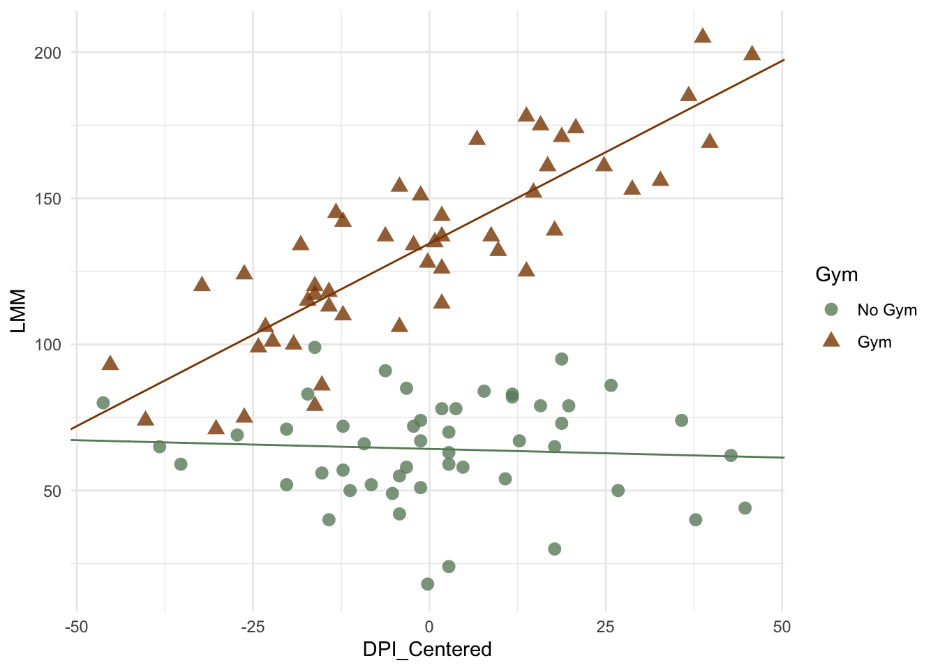
Let’s also plot the data to look at it’s functional form:
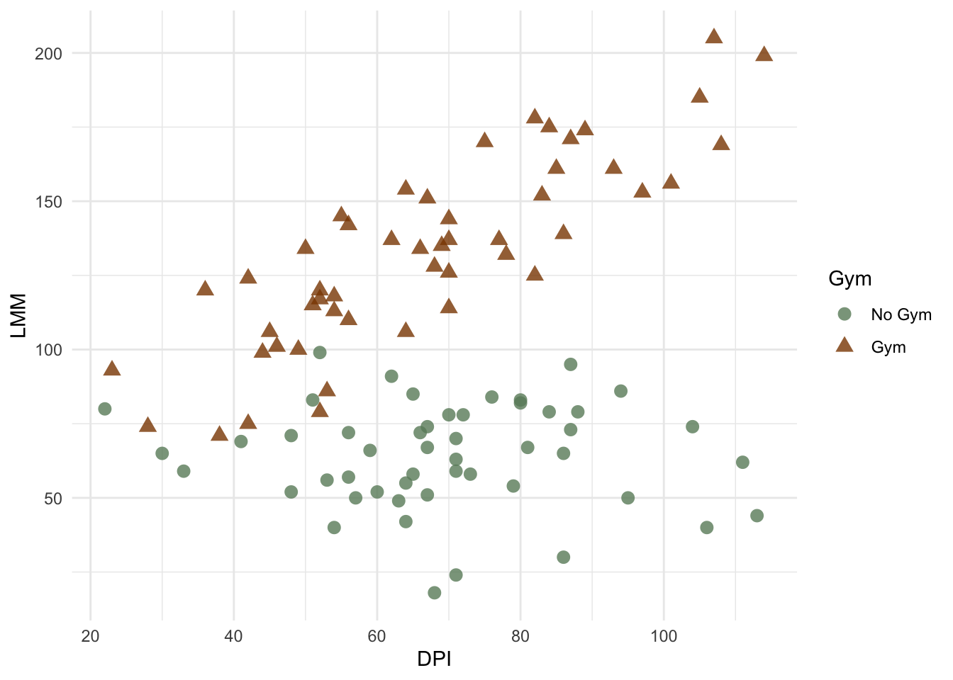
After looking at the plot, do you notice anything? Look closely at the potential relationship between DPI and LLM; does it differ for gym goers versus non-gym goers?
Let’s work out the equation for gym goers and non-gym goers separately using the results of the regression. Recall that this is our model:
\(y_{lmm}=b_o+b_{dpi}(x_{i1})+b_{gym}(x_{i2})+e_i\)
And these are our results:
Regression results using LMM as the criterion


   Predictor       b       b_95%_CI sr2 sr2_95%_CI             Fit
 (Intercept)  17.72*  [1.55, 33.89]
         DPI  0.67**   [0.45, 0.88] .10 [.03, .17]
      GymGym 70.45** [61.66, 79.23] .67 [.55, .79]
                                                       R2 = .743**
                                                   95% CI[.65,.80]


Note. A significant b-weight indicates the semi-partial correlation is also significant.
b represents unstandardized regression weights.
sr2 represents the semi-partial correlation squared.
Square brackets are used to enclose the lower and upper limits of a confidence interval.
* indicates p < .05. ** indicates p < .01.
The equation for non-gym goers is:
- Non-gym Goers (\(x_2=0\))
- \(y_{lmm}=17.72+0.67(x_{i1})+ 70.45(0)+e_i\)
- \(y_{lmm}=17.72+0.67(x_{i1})+e_i\)
While the equation of gym goers is:
- Gym Goers (\(x_2=1\))
- \(y_{lmm}=17.72+0.67(x_{i1})+70.45(1)+e_i\)
- \(y_{lmm}=88.17+0.67(x_{i1})+e_i\)
Let’s plot those lines on our previous figure:
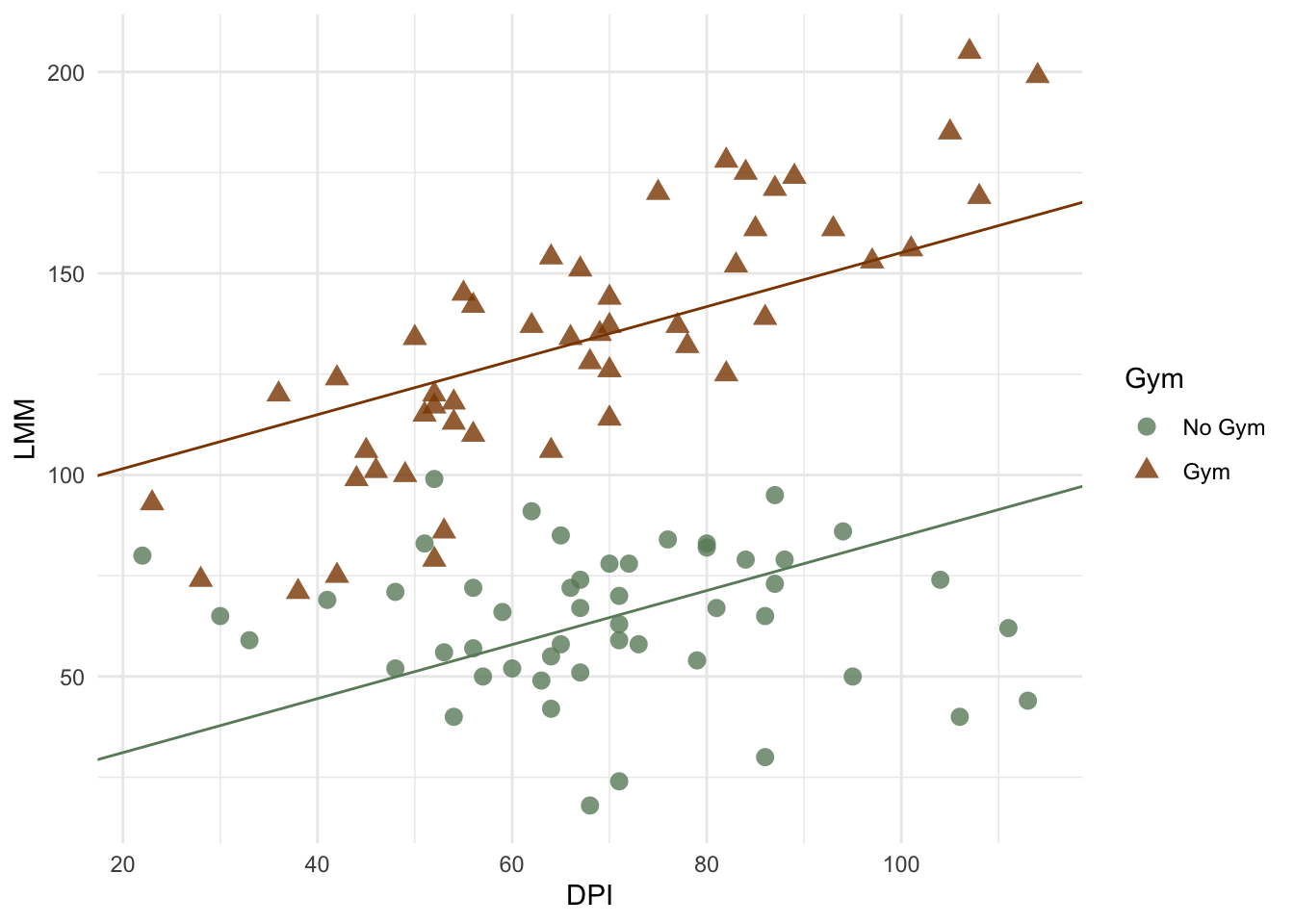
So, when we inspect the lines of best fit for each level of our gym variable, we notice something strange happening. The points on the no gym line seem to be above the line for lower DPI, but below the line for the higher DPI. The reverse trend may be evident in the ‘gym’ line. Thus, if we allowed these lines to have different slopes, perhaps they would fit better. Modelling an interaction (or moderation) allows us to do this.
16.4 Moderation
But first…
16.4.1 Multicollinearity
Remember that an assumption of multiple regression is the independence of our independent variables. To REDUCE multicollinearity, we must center our continuous predictors. You can center predictors by calculating the mean of a variable and then subtracting the mean from each individual’s score.
For example, imagine we measure confidence in five people and get these scores:
| Name | Confidence |
|---|---|
| Jessica | 17 |
| Haley | 8 |
| Letyraial | 13 |
| Alec | 10 |
| Zainab | 10 |
The mean of the confidence scores is 11.6. Thus, we will subtract each score by 11.6 to get the mean centered variable.
| Name | Confidence | Confidence Centered |
|---|---|---|
| Jessica | 17 | 5.4 |
| Haley | 8 | -3.6 |
| Letyraial | 13 | 1.4 |
| Alec | 10 | -1.6 |
| Zainab | 10 | -1.6 |
Let’s see how using centered predictors impacts the correlations between variables and reduces multicollinearity. Consider two different variables, x1 and x2, that are correlated:
    x1  x2
x1 1.0 0.2
x2 0.2 1.0
You can see they correlated, \(r=.20\). Let’s multiply them together to create an interaction term (x3, which is \(x_3=x_1\times x_2\)) and see how correlated each predictor is with the interaction term.
             x1      x2     x1_x2
x1    1.0000000 0.20000 0.9108277
x2    0.2000000 1.00000 0.5719200
x1_x2 0.9108277 0.57192 1.0000000
Now, let’s center x1 and x2 and create a new interaction term.
            x1         x2      x1_x2
x1    1.000000 0.20000000 0.21388102
x2    0.200000 1.00000000 0.06792511
x1_x2 0.213881 0.06792511 1.00000000
Notice how the correlations between the interaction term and each original term is reduced, or attenuated. For example, the correlation between x2 and the interaction term, x1_x2, was about \(r=.572\). The correlation between the centered x2 and the interaction term was \(r=.068\). Also notice that the correlation between centered and uncentered independent variables (not the interaction term) does not change!
So, for our main DPI and LMM example, we would center all continuous independent variables: DPI. We would model an interaction by creating a new variable (\(x_3\)=interaction) that is the product of the other variables (\(x_1=DPI\), \(x_2=gym\)) - \(x_3=(x_1)(x_2)\)
Let’s run our new model with centered interaction terms.
| Observations | 100 |
| Dependent variable | LMM |
| Type | OLS linear regression |
| F(3,96) | 166.84 |
| R² | 0.84 |
| Adj. R² | 0.83 |
| Est. | 2.5% | 97.5% | t val. | p | VIF | |
|---|---|---|---|---|---|---|
| (Intercept) | 64.27 | 59.32 | 69.21 | 25.80 | 0.00 | NA |
| DPI_Centered | -0.06 | -0.31 | 0.20 | -0.44 | 0.66 | 2.25 |
| GymGym | 70.27 | 63.28 | 77.27 | 19.95 | 0.00 | 1.00 |
| DPI_Centered:GymGym | 1.31 | 0.97 | 1.66 | 7.57 | 0.00 | 2.24 |
| Standard errors: OLS |
Let’s work out the equations again using the new model:
- No Gym (\(x_2=0\))
- \(y_{lmm}=64.27-0.06(x_{i1cent})+70.27(x_{i2})+1.31(x_{i1cent})(x_{i2})+e_i\)
- \(y_{lmm}=64.27-0.06(x_{i1cent})+70.27(0)+1.33(x_{i1cent})(0)+e_i\)
- \(y_{lmm}=64.27-0.06(x_{i1cent})+e_i\)
- Gym (\(x_2=1\))
- \(y_{lmm}=64.27-0.06(x_{i1cent})+70.27(x_{i2})+1.31(x_{i1cent})(x_{i2})+e_i\)
- \(y_{lmm}=64.27-0.06(x_{i1cent})+70.27(1)+1.31(x_{i1cent})(1)+e_i\)
- \(y_{lmm}=(64.27+70.27)-(0.06(x_{i1cent})+1.31(x_{i1cent}))+e_i\)
- \(y_{lmm}=134.54+1.25(x_{i1cent})+e_i\)
And a new visualization of our plot:
Notice how the new lines, with each group having their own intercept and slope seem to fit better. This is corroborated by the formal analysis, which resulted in the interaction being statistically significant (\(p<.001\)).
There is also a package in R that allows for 3D models of interactions. Have a look (you can interact with this figure) and try to understand what’s happening (note that the line of best fit becomes a ‘plane’ of best fit):
16.4.2 Continuous x Continuous Variable Interaction
We often will deal with multiple continuous variables that may interact. Fortunately, the process is similar. However, we will now need to center all predictors in the interaction.
Let’s stick to a similar example. Assume we want to determine if LMM regresses on DPI. But, we think that average hours in the gym per week will interact with protein intake to predict lean muscle mass. So, our previous categorical predictor of being a gym goer versus not is not a continuous predictor of average hours in the gym per week. So, we reach out to people and ask to now consider the average gym hours per week.
Our specific hypotheses are as follow:
16.5 Our Hypotheses
- DPI will predict LMM
- \(H1: \beta_{1}\ne0\)
- Average gym hours will predict LMM
- \(H2: \beta_{2}\ne0\)
- There will be an interaction between DPI and gym hours on LMM. Specifically, the relationship between DPI and LMM will be stronger for those who average more gym hours per week.
- \(H3: \beta_{3}\ne0\)
16.5.1 Our Data
Click to reveal the data
| ID | DPI | Gym | LMM |
|---|---|---|---|
| 31 | 27 | 5 | 198 |
| 38 | 29 | 3 | 165 |
| 24 | 36 | 4 | 183 |
| 1 | 39 | 5 | 192 |
| 39 | 39 | 4 | 157 |
| 7 | 42 | 1 | 141 |
| 26 | 42 | 7 | 309 |
| 9 | 45 | 7 | 337 |
| 22 | 45 | 6 | 289 |
| 28 | 45 | 3 | 201 |
| 40 | 45 | 5 | 219 |
| 5 | 47 | 3 | 139 |
| 34 | 47 | 3 | 213 |
| 49 | 47 | 6 | 228 |
| 35 | 48 | 6 | 257 |
| 36 | 48 | 3 | 198 |
| 3 | 49 | 4 | 241 |
| 33 | 49 | 2 | 185 |
| 4 | 50 | 3 | 200 |
| 27 | 50 | 6 | 240 |
| 16 | 52 | 4 | 268 |
| 23 | 52 | 5 | 315 |
| 42 | 52 | 5 | 213 |
| 12 | 53 | 7 | 294 |
| 18 | 54 | 6 | 329 |
| 44 | 54 | 10 | 402 |
| 6 | 55 | 7 | 393 |
| 21 | 55 | 4 | 176 |
| 41 | 55 | 6 | 295 |
| 48 | 55 | 6 | 360 |
| 19 | 56 | 2 | 178 |
| 14 | 57 | 2 | 192 |
| 25 | 57 | 6 | 271 |
| 32 | 57 | 6 | 260 |
| 13 | 58 | 7 | 319 |
| 8 | 60 | 4 | 285 |
| 10 | 63 | 3 | 192 |
| 17 | 63 | 5 | 298 |
| 2 | 64 | 5 | 255 |
| 15 | 66 | 4 | 271 |
| 20 | 66 | 5 | 358 |
| 43 | 66 | 1 | 191 |
| 29 | 70 | 5 | 347 |
| 46 | 70 | 5 | 323 |
| 37 | 72 | 6 | 399 |
| 30 | 73 | 4 | 246 |
| 11 | 74 | -1 | 5 |
| 45 | 76 | 7 | 396 |
| 50 | 76 | 6 | 298 |
| 47 | 98 | 5 | 430 |
16.6 Our Results
Our analysis results in the following:
| Observations | 50 |
| Dependent variable | LMM |
| Type | OLS linear regression |
| F(3,46) | 67.30 |
| R² | 0.81 |
| Adj. R² | 0.80 |
| Est. | 2.5% | 97.5% | t val. | p | VIF | |
|---|---|---|---|---|---|---|
| (Intercept) | 256.62 | 246.04 | 267.20 | 48.82 | 0.00 | NA |
| DPI_Centered | 2.75 | 1.92 | 3.57 | 6.69 | 0.00 | 1.01 |
| Gym_Centered | 31.73 | 26.14 | 37.33 | 11.41 | 0.00 | 1.04 |
| DPI_Centered:Gym_Centered | 0.70 | 0.22 | 1.18 | 2.93 | 0.01 | 1.05 |
| Standard errors: OLS |
Remember, the intercept here is for when all other variables are 0. However, we have centered our variables, so 0 carries a different meaning. Because we mean-centered, a score of 0 on a mean-centered variable is equal to the mean. So, the intercept in these results reflect the expected LMM score for an individual with an average DPI and Gym hours. We could expect someone who consumes the mean amount of protein and who goes to the gym an average amount of time to be 256.6237554.
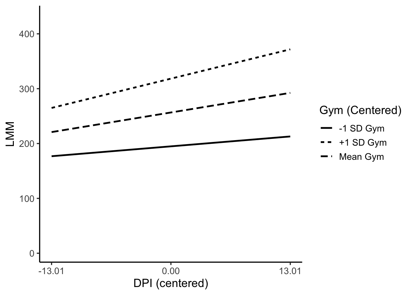
Let’s visualize the new interaction.
Or in 3D:
16.7 Our Write up
Let’s write up the results of this last model.
We regressed individual’s lean muscle mass (LMM) onto their daily protein intake (DPI), average hours or gym per week, and the interaction between DPI and Gym hours. The results suggest that DPI was a statistically significant predictor and accounted for 18% of the variance in LMM, \(b=2.75, p<.001, sr^2=.18, 95\%CI[.06, .30]\). Gym hours was a statistically significant predictor of and accounted for an addition 53% of the variance in LMM, \(b=31.73, p<.001, sr^2=.53, 95\%CI[.33, .72]\). Finally, the interaction between DPI and Gym hours was statistically significant and accounted for an addition 3% of the variance in LMM, \(b=0.70, p=.01, sr^2=.03, 95\%CI[-.01, .08]\).
16.8 Simple Slopes
Simple slopes analysis tests whether the slope (coefficient) of one predictor (i.e., one IV) differs from 0 at given levels or values of the moderator (i.e., another IV). Although we can you any level of value on the moderator, the typically convention if to test at -1SD, 0, and +1SD on the moderator. Thus, if a variable has a mean of 20 and SD of 10, then our simple slopes analysis will test if the slope for the IV and DV is statistically significant for the values 10, 20, and 30 on the moderator.
These analyses can be used to provide additional information about a potential interaction. Let’s use the data from our last example and run a simple slopes analysis.
SIMPLE SLOPES ANALYSIS

Slope of DPI when Gym = 2.715778 (- 1 SD):

  Est.   S.E.   t val.      p
------ ------ -------- ------
  1.39   0.59     2.36   0.02

Slope of DPI when Gym = 4.660000 (Mean):

  Est.   S.E.   t val.      p
------ ------ -------- ------
  2.75   0.41     6.69   0.00

Slope of DPI when Gym = 6.604222 (+ 1 SD):

  Est.   S.E.   t val.      p
------ ------ -------- ------
  4.11   0.65     6.31   0.00
As is seen from the output, we are given a separate analysis for each value of the simple slopes analysis. In this specific example, the relationship between DPI and LMM was statistically significant at all tested levels (-1SD, mean, and +1SD) of gym hours.