14 Simple Regression

14.1 Background Information

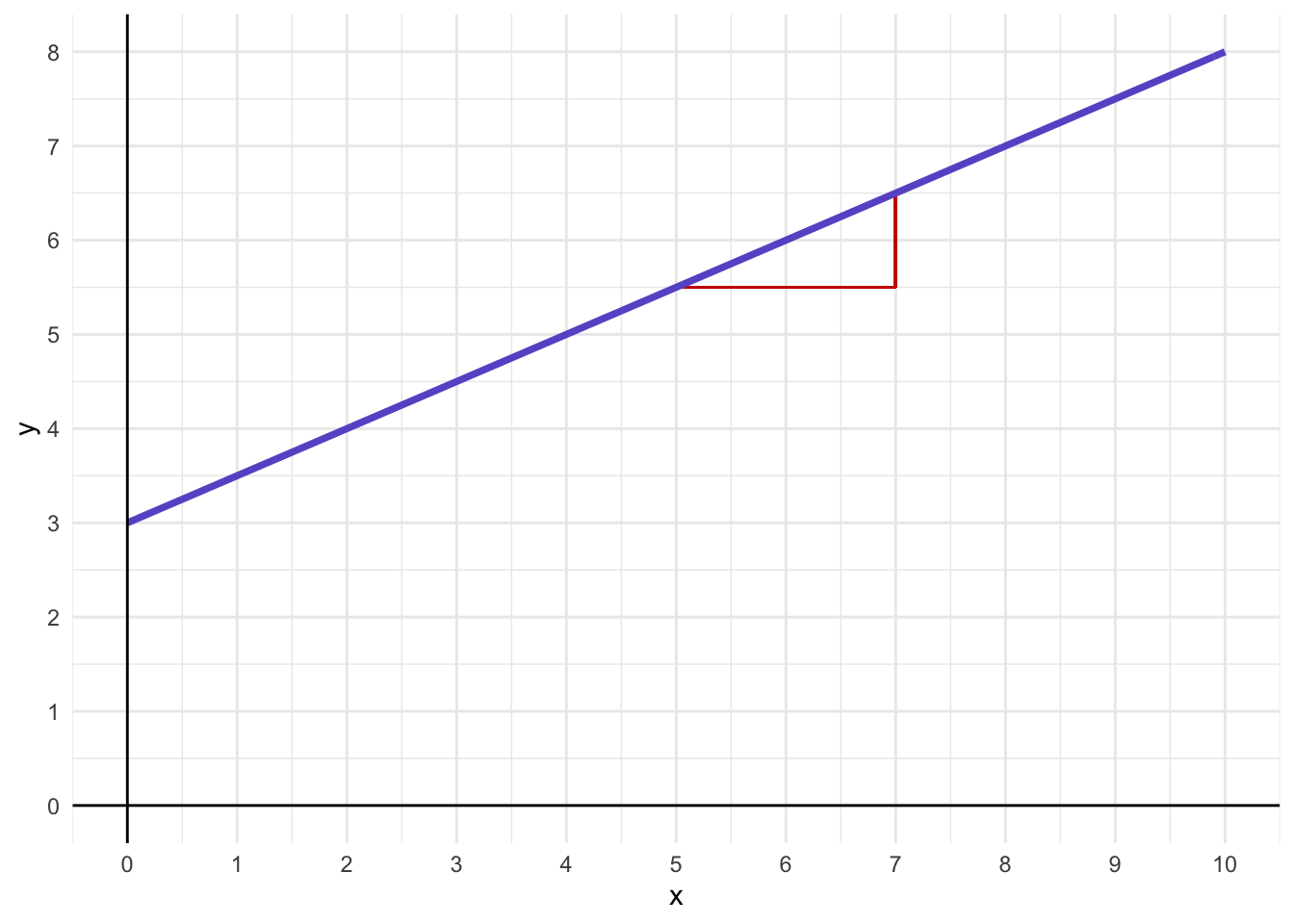
Prior to diving into the data, let’s revisit some high school math! You likely recall \(y=mx+b\), the function of a line. Recall that we can determine the y-position of a line by knowing the x position, the slope, and the y-intercept of that line. Consider the following:

Hopefully, you can see that the line crosses the y-axis at 3. Furthermore, the slope can be calculated by \(\frac{y_2-y_1}{x_2-x_1}\) or, rise over run. This is represented by the red lines. Using rise over run, we get: \(\frac{6.5-5.5}{7-5}=\frac{1}{2}=0.5\). Thus, the above line is represented by \(y=0.5x+3\). We can readily predict what the value of y would be by knowing the value of x. For example, by knowing that \(x=3\), we could determine that \(y\) is \(y=0.5x+3=0.5(3)+3=4.5\).

Practice Question

Determine the equation for the following line:

Answer

\(y = -1x+9\)

You may be thinking, “STOP TYLER”, but this is relevant. This equation maps nicely onto our more general linear model that we use for our analyses:

\(y_i = model+e_i\)

Where \(y_i\) is the outcome for individual i, the model is based on our hypotheses and resulting analyses, and \(e_i\) is the error for individual i (i.e., what the model does not explain).

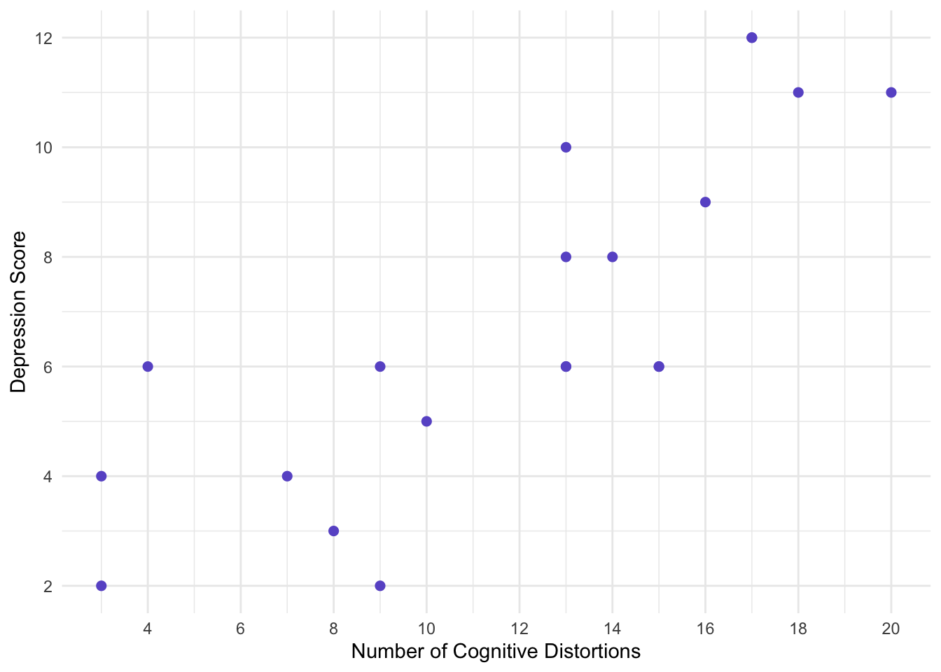
Imagine that instead of x and y, we had a independent and a dependent variable. Say, we wanted to predict someones depression score (y; and measured on a scale of 1-14) by knowing the number of cognitive distortions they have on average each day. It might look like the following:

We can try to fine a straight line that fits all those points, but it won’t be able to. For example, maybe we can guess that that y-intercept is around 2.5, and the slope is about 0.5. This would result in:

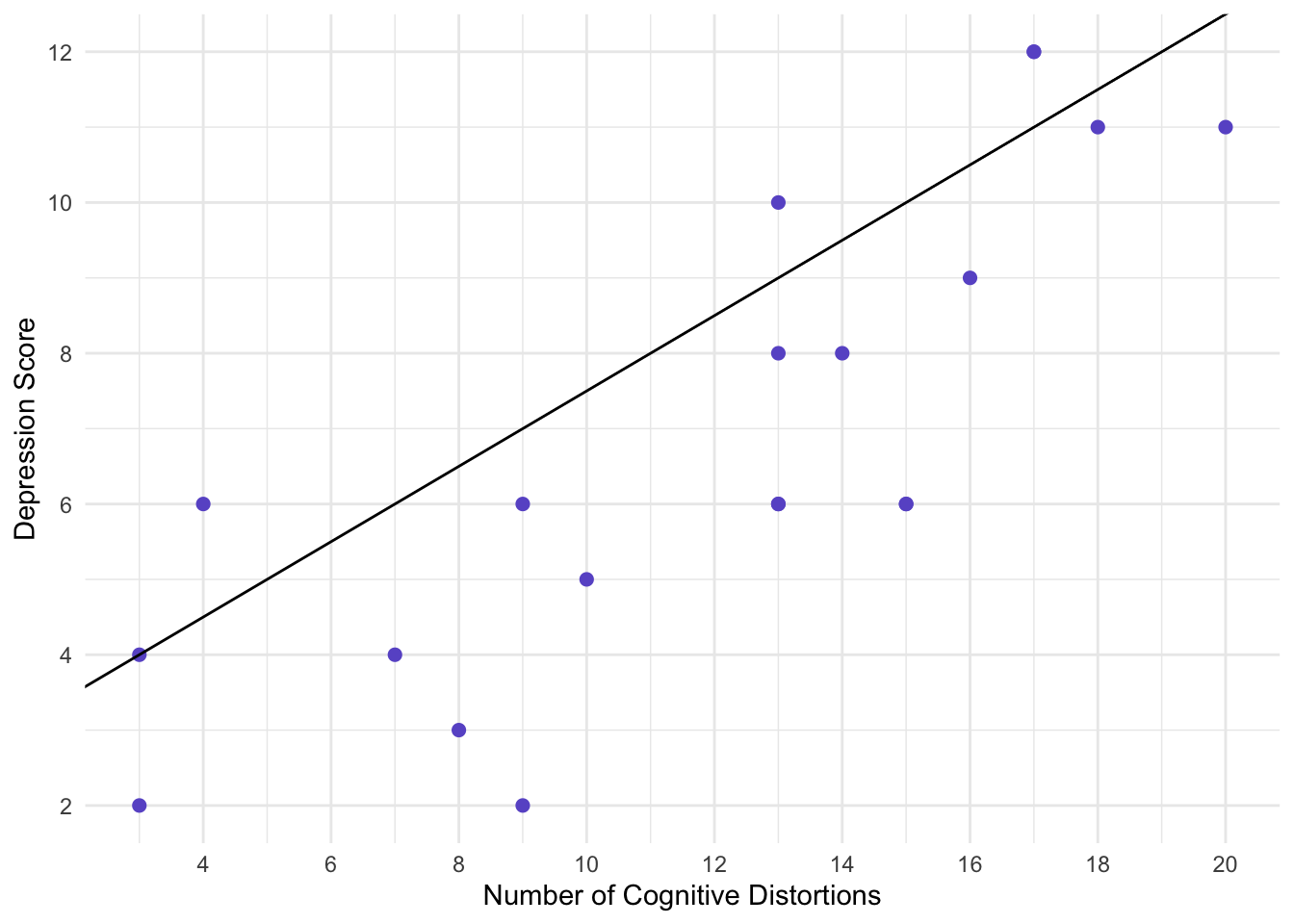
That’s not too bad of a guess…but what it seems to have a lot of error.

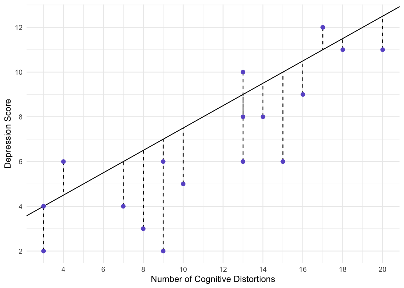
Here, error is represtned by the dotted lines. That is, we guessed that:

\(dep=2.5+0.5(Distortions)\)

But that would mean that the points fall directly on the line. Thus, the distance between each point and the line is the error. Let’s consider person 1 (circled below).

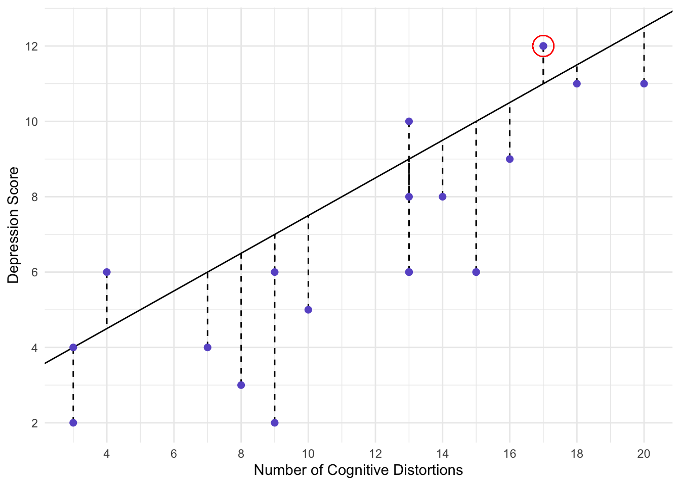
This person had, on average, 17 cognitive distortions per day and had a depression score of 12. Our line would not predict a depression score of 12.

\(depression=2.5+0.5(distortions)=2.5+0.5(17)=11\)

The difference between 12 and 11 is the error for individual 1. We typically call this a residual. The residual for individual 1 is 1.

\(y_i=2.5+0.5(x_i)+e_i\)

For person 1:

\(12=2.5+0.5(17)+1\)

Hmmm. I wonder if we could find a better fitting line, that would minimize the errors across all the observations? That is, if we calculated the error for every person, as we did for person 1, the total of the squared errors would be 115.75. We can get this number lower.

14.1.1 Ordinary Least Squares

Ordinary Least Squares (OLS) is an algebraic way to get the best possible solution for our regression line. It minimizes the error of the line. Typically in psychology we write a simple regression as the following:

\(y_i=b_0+b_1x_i+e_i\)

Where \(\hat{y}\) is the predicted score on y, the dependent variable, \(b_0\) is the intercept, \(b_1\) is the slope, \(x_1\) is the score of individual i on the independent variable, and \(e_i\) is the residual for individual i.

The following are solutions to OLS simple regression:

\(b_1=\frac{cov_{(x, y)}}{s^2_{x}}\)

Where \(cov_{(x, y)}\) is the covariance between x and y, and \(s^2_x\) is the variance of x. For us:

\(b_1=\frac{12.87105}{25.29211}=0.50889\)

And the intercept solution is:

\(b_0=\overline{y}-b_1\overline{x}\)

Therefore:

\(b_0=6.85-0.50889(11.85)=0.81965\)

You did it! Our best possible fitting line is:

\(y_i=0.81965+0.50889(x_i)+e_i\)

If we were to calculate the sum or the squared residuals for each person, we would get 66.1. This is much lower than the line that was built on our best guess.

Typically, when using regression, research reference trying to predict some variable using another variable. The predictor is often the independent variable (x), and the outcome/criterion variable is the dependent variable (y). When we have only one predictor, we refer to this as a simple regression. Note: this is not way implies that x causes y. Consider prediction much like a relationship or association, as discussed in the last chapter on correlations.

14.2 Our Data

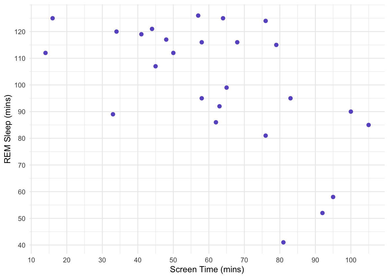
You are a psychologist investigating the impact of technology use at night and sleep quality. Specifically, you believe that the amount of screen time within two hours of bedtime will negatively impact the total time in REM sleep. You recruit students and ask them to measure both screen time before bed (IV) and access their Apple Watch data to assess the amount of time in REM sleep during the night (DV).

14.2.1 Power

You review the literature and believe that the link between screen time and sleep is negative. Specifically, your best guess at the population parameter is \(R^2=.25\), which can be converted to \(f^2=.3333\) (\(f^2=\frac{R^2}{1-R^2}\). We will conduct a power analysis. For simple regression, the degrees of freedom for the numerator is \(n_b-1\). Note that you must include the intercept! So our \(df_{numerator}=2-1=1\). The power analysis is as follows:

pwr.f2.test(f2=.3333, 
            power=.8,
            u=1)


     Multiple regression power calculation 

              u = 1
              v = 23.6195
             f2 = 0.3333
      sig.level = 0.05
          power = 0.8

So, the results suggest that \(v=23.62\). We will round to \(24\). But what does this mean? The degrees of freedom, v, can is: \(df_{denominator}=N-n_b\). Thus:

\(24=N-2\) can be rearranged to \(N=24+2=26\). Thus, we recruit 26 individuals. Our data is as follows:

Click to reveal/hide

Screen Time	REM Sleep
64	125
79	115
50	112
83	95
48	117
45	107
63	92
14	112
57	126
92	52
62	86
16	125
34	120
68	116
76	124
100	90
41	119
76	81
105	85
58	116
33	89
81	41
65	99
44	121
58	95
95	58

14.3 Our Hypothesis

Regression will focus on \(b\)s (betas), which are regression coefficients. Thus, our hypothesis (we will use two-tailed) is:

\(H_0:b=0\); and

\(H_A:b\neq0\)

14.4 Our Model

Recall that we started by relating our regression to \(y=mx+b\), specifically:

\(outcome_i=(model)+error_i\)

And we are hypothesizing that the outcome is the function of some variables, so we can now say:

\(y_i=b_0+b_1(x_{1i})+e_i\)

Where \(y_i\) is the DV for individual i, \(b_0\) is the intercept, \(b_1\) is the coefficient for the IV, and \(e_i\) is the residual for individual i.

14.5 Our Analysis

We can use the formulas above to solve the regression equation. We will need the mean of the IV (Screen Time), mean of the DV (REM Sleep), their covariance, and the variances. These are as follows:

Mean_Screen	Mean_REM	Var_Screen	Var_REM	Cov
61.80769	100.6923	572.4015	548.8615	-321.3015

Thus:

\(b_1=\frac{cov_{(ST, REM)}}{s^2_{ST}}= \frac{-321.3015}{572.4015}=-0.5613\)

We interpret this as, for every unit change in Screen Time (which was in minutes), we would predict a 0.5613 unit decrease in REM sleep. Thus, for every minute more of screen time, we would predict 0.5613 less minutes of REM sleep.

We must also solve for \(b_0\).

\(b_0=\overline{y}-b_1\overline{x} = 100.6923 -61.80769 (-0.5613)=135.385\)

The interpretation of this is: we would predict someone with NO screen time before bed (\(x=0\)) to get 135.34 minutes of REM sleep. Note: sometimes it makes no sense to interpret the intercept. For example, imagine regression weight onto height. We would interpret an intercept as ’we would predict a height of XXX for someone with NO weight; that doesn’t make sense!

We have our final equation!

\(y_i=135.39+(-0.561)(x_i)+e_i\)

14.5.1 Effect Size

Effect size for simple regression is \(R^2\), which is interpreted as teh amount of variance in the outcome that is explained by the model. Since we have only one predictor, \(R^2\) is simply the squared coreraltion between the one IV and the DV. The correlation between Screen Time and REM Sleep is -0.5732328. Thus:

\(R^2=(r)^2=(-0.5732328)^2=0.329\)

Therefore, the model explains 32.9% of the variance in REM Sleep.

14.5.2 Analysis in R

Regression and ANOVAs fall under the ‘general linear model’, which indicates that an outcome (e.g., \(y_i\), DV) is the function of some linear combination of predictors (e.g., \(b_1(x_i)\)). We can use the lm() (linear model) function to write out our regression equation.

lm(REM ~ ScreenTime, data=sr_data)

Note that here, I have a data frame called sr_dat with two variables called ScreenTime and REM. The ~ symbol is the same as ‘equal’ or predicted by. So, we have REM is predicted by ScreenTime. R will automatically include an intercept and the error term.

The results of lm(REM ~ ScreenTime, data=sr_data) should be passed into a summary() argument. So, first, let’s create our model!

our_model <- lm(REM ~ ScreenTime, data=sr_dat)

And then pass that into the summary function:

summary(our_model)


Call:
lm(formula = REM ~ ScreenTime, data = sr_dat)

Residuals:
    Min      1Q  Median      3Q     Max 
-48.919 -10.800   4.189  10.637  31.274 

Coefficients:
            Estimate Std. Error t value Pr(>|t|)    
(Intercept) 135.3863    10.8277  12.504 5.31e-12 ***
ScreenTime   -0.5613     0.1638  -3.427   0.0022 ** 
---
Signif. codes:  0 '***' 0.001 '**' 0.01 '*' 0.05 '.' 0.1 ' ' 1

Residual standard error: 19.59 on 24 degrees of freedom
Multiple R-squared:  0.3286,    Adjusted R-squared:  0.3006 
F-statistic: 11.75 on 1 and 24 DF,  p-value: 0.002205

14.5.3 Another Way

The apaTables package also has a lovely output, and can save a word document with the output.

library(apaTables)
apa.reg.table(our_model)



Regression results using REM as the criterion
 

   Predictor        b         b_95%_CI  beta    beta_95%_CI sr2 sr2_95%_CI
 (Intercept) 135.39** [113.04, 157.73]                                    
  ScreenTime  -0.56**   [-0.90, -0.22] -0.57 [-0.92, -0.23] .33 [.05, .55]
                                                                          
                                                                          
                                                                          
      r             Fit
                       
 -.57**                
            R2 = .329**
        95% CI[.05,.55]
                       

Note. A significant b-weight indicates the beta-weight and semi-partial correlation are also significant.
b represents unstandardized regression weights. beta indicates the standardized regression weights. 
sr2 represents the semi-partial correlation squared. r represents the zero-order correlation.
Square brackets are used to enclose the lower and upper limits of a confidence interval.
* indicates p < .05. ** indicates p < .01.

While the regular lm() function gives exact p-values, the apa.reg.table() function gives more info such as CIs, r, sr, and effect size.

14.6 Our Results

We fitted a linear model to predict REM Sleep with Screen Time. The model explains a statistically significant and substantial proportion of variance, \(R^2 = 0.33\), \(F(1, 24) = 11.75\), \(p = 0.002\). Screen Time was a statistically significant and negative predictor of REM sleep, \(b = -0.56\), \(95\%CI[-0.90,-0.22]\), \(t(24) = -3.43\), \(p = 0.002\).

14.7 Our Assumptions

There are a few basic assumptions:

Homoscedasticity

The residual variance is constant across different levels/values of the IV. R can produce a plot of residuals across each fited value of \(y\).

plot(our_model, 1)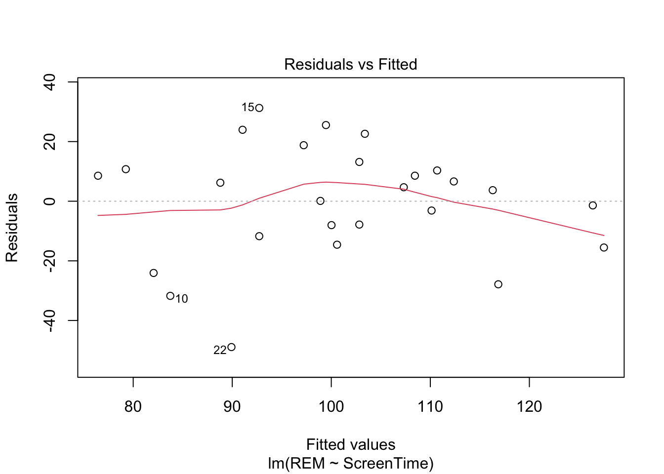

Here, we want a relatively straight line around 0, indicating an mean residual of 0. Furthermore, we want the dots to be dispersed equally around each fitted value. It’s hard to determine with our data because there are so few points.

Independence

Each observation is independent; thus, each residual is independent. You must ensure this as a researcher. For example, if you had repeated measures (e.g., two observation from each person), then these would not be independent.

Linearity

The relationship between IV and DV is linear. We can visually assess this using a scatterplot. We hope that the points seem to follow a straight line. We can fit our line of best fit from OLS to help with this.

`geom_smooth()` using formula 'y ~ x'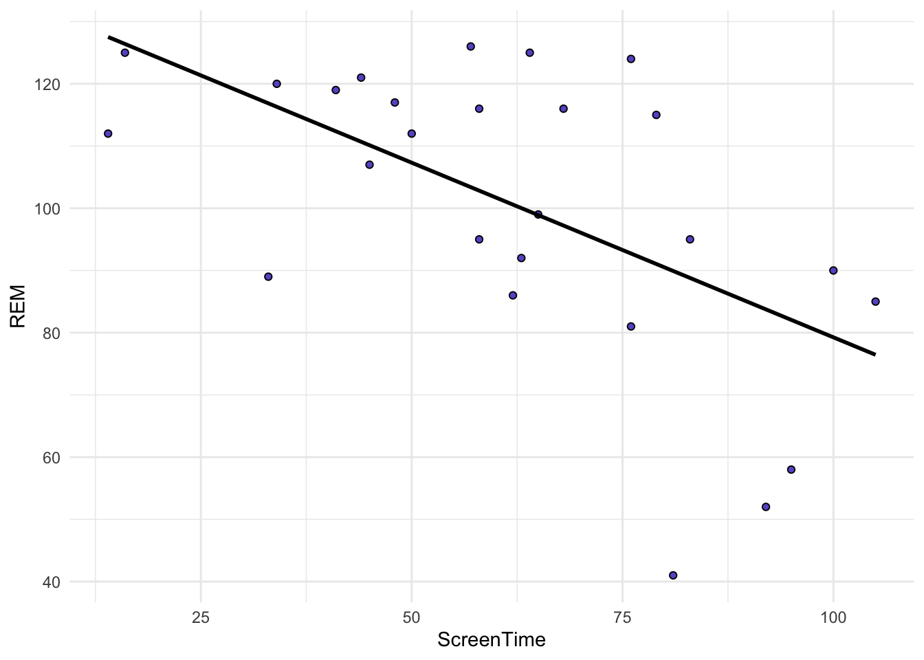

Our data appear quite linear. Some examples of non-linear plots:

Quadratic

`geom_smooth()` using formula 'y ~ x'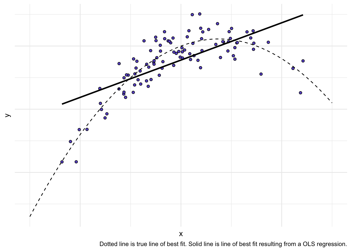

Normality of residuals

We can asses using Q-Q plots and Shapiro-Wilk, which was covered in a previous chapter. Remember, the null hypothesis of the SW test is that the data are normally distributed.

qqnorm(our_model$residuals)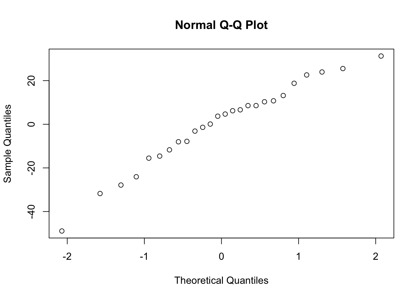

shapiro.test(our_model$residuals)


    Shapiro-Wilk normality test

data:  our_model$residuals
W = 0.96592, p-value = 0.5211

14.8 Practice Question

Practice Question

Generate the regression equation for the following data that investigating the Graduate Record Exams ability to predict GPA in graduate school.
Interpret the intercept and coefficient for GRE.
Write the hypotheses.
Write up the results.

Student	GRE	GPA
1	163	1.6
2	171	1.9
3	173	1.8
4	139	3.1
5	174	3.9
6	139	1.7
7	162	1.6
8	141	3.6

Answers


Call:
lm(formula = GPA ~ GRE, data = dat_prac)

Residuals:
    Min      1Q  Median      3Q     Max 
-0.9105 -0.7439 -0.3900  0.6201  1.6824 

Coefficients:
            Estimate Std. Error t value Pr(>|t|)
(Intercept)  4.17081    3.94968   1.056    0.332
GRE         -0.01123    0.02493  -0.450    0.668

Residual standard error: 1.028 on 6 degrees of freedom
Multiple R-squared:  0.03268,   Adjusted R-squared:  -0.1285 
F-statistic: 0.2027 on 1 and 6 DF,  p-value: 0.6683

\(y_i=b_0+b_1(x_{1i})+e_i\)

\(y_i=-4.17+(-0.011)(x_{1i})+e_i\)

Intercept: Someone with a score of 0 on the GRE would be predicted to have a score GPA of 4.17 (this is impossible).

Slope: For every one unit increase in GRE score, we would predict a 0.011 unit dencrease in GPA.

\(H_0: b_1=0\)

\(H_A: b_1\neq0\)

We fitted a linear model to predict GPA with GRE. The model did not explain a statistically significant proportion of variance \(R^2 = 0.03\), \(95\%CI[.00,.41]\), \(F(1, 6) = 0.20\), \(p = 0.668\). The effect of GRE is statistically non-significant, \(b = -0.01\), \(95\% CI [-0.07, 0.05]\), \(t(6) = -0.45\), \(p = 0.668\).