6 NHST and Power

6.1 Null Hypothesis Significant Testing

Null hypothesis significance testing (NHST) is a controversial approach to testing hypotheses. It is the more employed approach in psychological science.

Simply, NHST begins with an assumption, a hypothesis, about some effect in a population. Data is collected that is believes to be representative of that population. Should the data not align with the null hypothesis, it is taken as evidence against the null hypothesis.

There are several concepts related to NHST and misconceptions that need to be addressed to facilitate your research.

6.2 p-values

Prior to exploring p-values, let’s ensure you have a basic understanding of probability notation. First, the notation:

$p (x)$ which would indicate the probability of $x$ .

For example, the probability of flipping a coin and getting a heads, $p (h e a d s) = .5$ . This indicates a 50% probability of getting a heads. Probability ranges from 0 (no chance), to 1 (guarantee). For example, the probability that you, the person reading this, is in Grenfell’s PSYC 3950 class is high. Thus, my best guess right now is that $p (3950 s t u d e n t) > .95$ . Hypothetically, if I could survey everyone who has read this sentence, I would expect 19 out of 20 of them to be in PSYC 3950. I would expect one of them not to be (e.g., someone randomly stumbled on this page…lucky you!).

Additionally, I could use the notation:

$p (x | y)$ which would indicate the probability of $x$ , given $y$ .

For example, what if I provided more details in the previous coin example: I say now that the coin is not a fair coin. Well, the original probability will only hold if the coin is fair. That is, p(heads|fair coin) = .5. However, with the new information, p(heads|unfair coin) $\neq$ .5.

Reserve probabilities are not equal. That is, $p (x | y) \neq p (y | x)$ . Consider the following: what is the probability that someone is Canadian, given that they are the prime minister of Canada: p(Canadian|Prime Minister)? Do you think this is equal to the probability that someone is the Prime Minister of Canada, given that they are Canadian: p(Prime Minister|Canadian)? I would argue that the former is $p = 1.00$ , while the later is not. In fact, the later can be calculated. Given there are about $38, 000, 000$ Canadians, and there is only one current Prime Minister, than the probability that someone is Prime Minister, given that they are Canadian p(Prime Minister|Canadian)= $\frac{1}{38, 000, 000}$ =.0000000263. So:

p(Canadian|Prime Minister) = 1.00
p(Prime Minister|Canadian)=.0000000263

A key feature of NHST is that the null hypothesis is assumed to be true. Given this assumption, we can estimate how likely a set of data are. This is what a p-value tells you.

The p-value is the probability of obtaining data as or more extreme than you did, given a true null hypothesis. We can use our notation:

$p (D | H_{0})$

Where D is our data (or more extreme) and $H_{0}$ is the null hypothesis.

When the p-value meets some predetermined threshold, it is often referred to as statistical significance. This threshold has typically, and arbitrarily been $α = .05$ . Should data be so unlikely that is crosses the threshold, we take it as evidence against the null hypothesis and reject it. If it is below the threshold, we fail to reject it. Note: we do not accept the null hypothesis. Liken this to a courtroom verdict, which is that someone is guilty or not guilty. A not guilty verdict does not mean that someone is innocent, it means there is not enough evidence to convict.

…beginning with the assumption that the true effect is zero (i.e., the null hypothesis is true), a p-value indicates the proportion of test statistics, computed from hypothetical random samples, that are as extreme, or more extreme, then the test statistic observed in the current study.

(Spence & Stanley, 2018)

or, stated another way:

The smaller the p-value, the greater the statistical incompatibility of the data with the null hypothesis, if the underlying assumptions used to calculate the p-value hold. This incompatibility can be interpreted as casting doubt on or providing evidence against the null hypothesis or the underlying assumptions.

(Wesserstein & Lazar, 2016)

Simply, a p-values indicates the probability of your, or more extreme, test statistic, assuming the null: $p (d a t a | n u l l)$ . For ease, consider the following table:

		Reality
		No Effect ( $H_{o}$ True)	Effect ( $H_{1}$ True)
Research Result	No Effect ( $H_{o}$ True)	Correctly Fail to Reject $H_{o}$	Type II Error ( $β$ )
	Effect ( $H_{1}$ True)	Type I Error ( $α$ )	Correctly Reject $H_{o}$

When we conduct NHST, we are assuming that the null hypothesis is indeed true, despite never truly knowing this. As noted, a p-value indicates the likelihood of your or more extreme data given the null.

6.2.1 If the null hypothesis is true, why would our data be extreme?

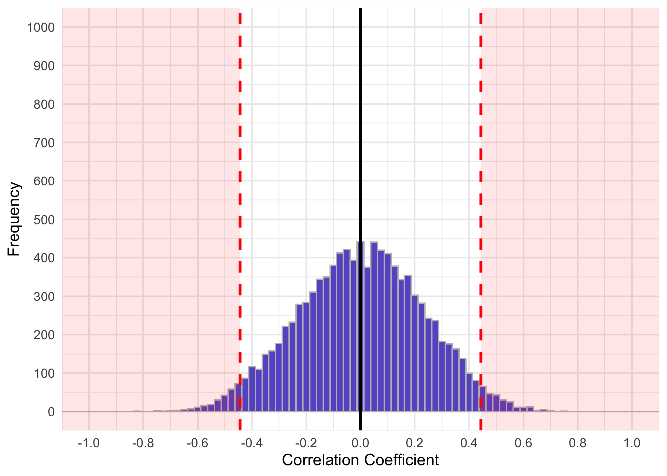
In inferential statistics we make inferences about population-level parameters based on sample-level statistics. For example, we infer that a sample mean is indicative of a population mean. In, NHST, we assume that population-level effects or associations (i.e., correlations, mean differences, etc.) are zero, null, nothing at a population level (note: this is not always the case). If we sampled from a population whose true effect or association was $0$ an infinite number of times, our sample statistics would form a distribution around the population parameter. Consider a population correlation of $ρ = 0$ . If we took infinite samples of size $n$ from this population, let’s say 20 people, we would get a distribution that looks something like:

The above shows the distribution of 10,000 correlation coefficients derived from simulated samples from a population that has $ρ = 0$ . Although not quite an infinity number of samples, I hope you get the idea. The red shaded region shows the two tails that encompass 5% of the samples (2.5% per tail). These extreme 5% are at the correlation coefficients, $r \geq .444$ or $r \leq - .444$ . Thus, there is a low probability of getting a correlation beyond $+ / - .444$ when the null hypothesis is true. If we ran a correlation test with sample $n = 20$ and $α = .05$ , a correlation of $r = .444$ would result in approximately $p = .05$ (the actual value of $p$ for $n = 20$ and $r = .44377$ is $p = .049996$ , but there are rounding errors). Because the probability of this data is quite low, given $H_{0} = 0$ , we often reject the null hypothesis. Our data is very unlikely given a true null hypothesis, therefore we reject the null.

The magnitude of the tails is arbitrary, for the most part, but has been set to a standard of 5% (corresponding $α = .05$ ) since the early 20th century, which is a further criticism of NHST. However, we set our $α$ threshold/criteria, and as show in the previous paragraph, our $α$ level influences the correlation coefficient we would consider statistically significant. Imagine we wanted to reduce out criteria, such that $α = .01$ . What do you think would happen to the red shaded region in the above graph and the critical correlation coefficient? If we wanted to adjust what we consider extreme so that it is less conservative, which is essentially what we are doing when we reduce our alpha, we would shift the red regions outward and our critical correlation coefficients would be larger in absolute magnitude. In this case, our graph would be:

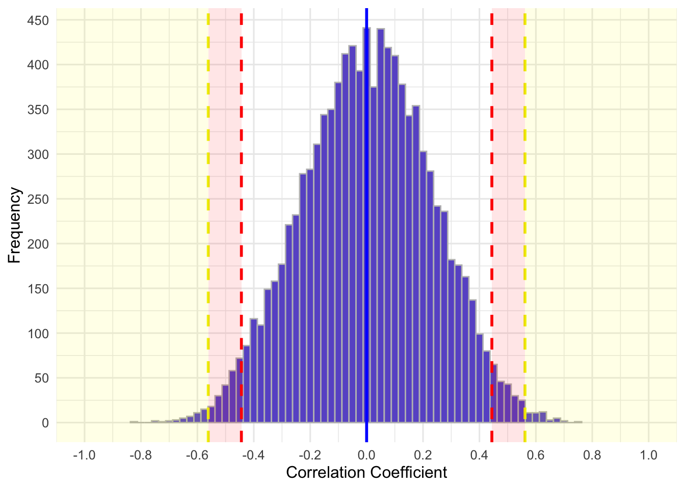
The yellow region represents the extreme 1% of the distribution (0.5% per tail). The red region is where the original regions were for $α = .05$ .The proportion of samples in the red region is? You guessed it, 4%. These 4% of samples have correlations, $.561 > r \geq .444$ . Remember, these are for a sample of $n = 20$ . The critical correlation coefficients differ based on sample size because they influence the standard errors (i.e., it gets skinnier or fatter).

So, we set the criterion of $α$ a priori and our resultant p-value let us decide if our data are probable given $H_{0}$ . If it’s lower than our criterion we can reject $H_{0}$ , suggesting only that the population effect is not zero. It is often called statistically significant. Otherwise, if our p-value is larger than our criterion, we decide that our data is not that unlikely and fail to reject that $H_{0}$ .

In short, p-values are the probability of getting a set of data or more extreme given the null. We compare this to a criterion cut-off, $α$ . If our data is very improbable given the null, so much that is is less than our proposed cutoff, we say it is statistically significant.

6.2.2 Misconceptions

Many of these misconceptions have been described in detail elsewhere (e.g., Nickerson, 2000). I visit only some of them.

6.2.2.1 Odds against chance fallacy

The odds against chance fallacy suggests that a p-value indicates the probability that the null hypothesis is true. For example, someone might conclude that if their $p = .04$ , there is a 4% chance that the null hypothesis is true. Above you learned that p-values indicate $p (D | H_{0})$ and that you cannot simply flip the conditional probabilities so that $p (H_{0} | D)$ . The p-value tells you nothing about the probability of a null hypothesis other than it is assumed true. Under a p-value, $p (H_{0}) = 1.00$ .

Jacob Cohen outlines a nice example wherein he compares $p (D | H_{0})$ to the probability of obtaining a false positive on a test of schizophrenia. Given his hypothetical example, the prevalence of schizophrenia and the sensitivity and specificity of assessment tests for schizophrenia, an unexpected result (a positive test) is more likely to be a false positive than a true negative. You can read his paper here.

If you want $p (H_{0} | D)$ , you may need another route such as Bayesian Statistics.

6.2.2.2 Odds the alternative is true

In NHST, no likelihoods are attributed to hypotheses. All p-values are predicated on $p (H_{0}) = 1.00$ . Thus, statements such as ‘1-p indicates the probability $H_{A}$ is true’ is itself false.

6.2.2.3 Small p-values indicate large effects

This is not the case. P-values depend on other things, such as sample size, that can lead to statistical significance for minuscule effect sizes. For example, one can achieve a high degree of statistical power (discussed below) for a population effect of $d = .01$ (Cohen’s d; this would be considered an extremely small effect).

Power ( $1 - β$ )	d ( $d$ )	Alpha ( $α$ )	Required Sample to Achieve Power	Cohen’s Effect Size Classification
.8	.02	.05	39,245	<Small
.8	.05	.05	6,280	<Small
.8	.2	.05	393	Small
.99	.02	.05	91,863	<Small

From the table above, if the true population effect was TINY, $d = .02$ , we would find a statistically significant effect 99% of the time if we sampled about 91,000 people. Thus, with a large enough sample we will obtain statistical significance for even tiny effects.

6.3 Power

Whereas p-values rest on the assumption that the null hypothesis is true, the contrary assumption, that the null hypothesis is false (i.e., an effect exists), is important for determining statistical power. Statistical power is defined as the probability of correctly rejecting the null hypothesis given an true population effect size and sample size, or more formally:

Statistical power is the probability that a study will find p < $α$ IF an effect of a stated size exists. It’s the probability of rejecting $H_{0}$ when $H_{1}$ is true. (Cumming & Calin-Jageman, 2016)

See the following figure for a depiction, where alpha= $α$ and 1-beta = $1 - β$ = power:

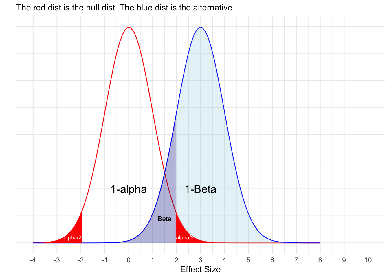
We can conclude from this definition that if your statistical power is low, you will not likely reject $H_{0}$ regardless of if there is a population-level effect (i.e., $H_{0} \neq 0$ ). As will be shown, underpowered studies are doomed from the start. Conversely, if a study is overpowered (i.e., extremely large sample size), you can get a statistically significant result for what might be a infinitesimal or meaningless effect size.

Before proceeding to the next example, please note that you will often see the symbol ‘rho’, which is represented by the Greek symbol $ρ$ (it’s a blend of r and o). This is the population parameter of a correlation. This is the not the same as a p-value, which is represented by the letter $p$ . It may get confusing it you mix up these symbols, so be sure you know the difference between the two.

Consider a researcher who is interested in the association substance use (SU) and suicidal behaviors (SB) in Canadian high school students. Let’s assume that the true association between SU and SB is $ρ = .3$ ; we do not know that this is the true value. The population data might look like this:

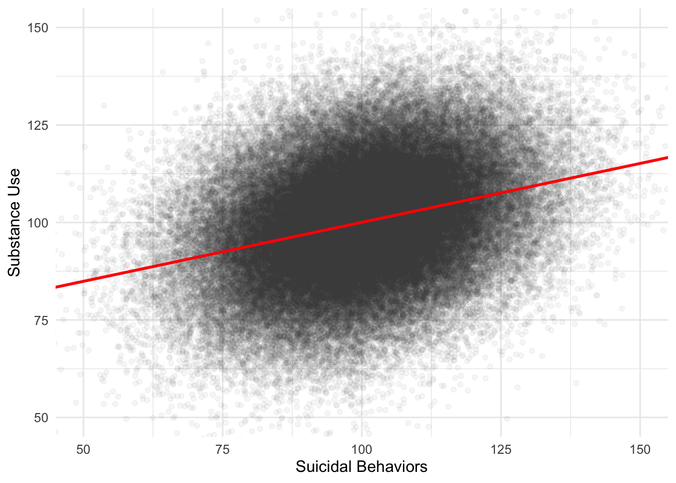
So, it appears that as substance use increases, so do suicidal behaviors. Although we aren’t so omniscient in the real world, the population correlation here is $ρ = .300$ . Note, “rho”, the population correlation uses the symbol $r h o$ , which is not the same as $p$ . We will use this known population correlation to determine the probability that our proposed study will correctly reject a null hypothesis, which, as you remember, states there is no relationship between SU and SB.

Before conducting our study, we will conduct a power analysis to determine an appropriate sample size required to adequately power our study. We want to have a good probability of rejecting the null, if it were false (here, we know this is the case). To calculate our required sample size, we require: i) our $α$ criterion level, ii) our desired power ( $1 - β$ ), and iii) our hypothesied effect size. We will use the standard for our $α$ criterion and power, i) $α = .05$ , ii) 1- $β$ = .8, and we know our true effect, iii) $ρ$ = .300. Although we know the population correlation, in real-world research we would need to find a good estimate of the effect size, which is typically through reading the literature for effect sizes in similar populations. We can use the pwr package to conduct our power analysis. This package is very useful; you can insert any three of the required four pieces of information to calculate the missing piece. More details on using pwr are below. For our analysis, we get:


     approximate correlation power calculation (arctangh transformation) 

              n = 84.07364
              r = 0.3
      sig.level = 0.05
          power = 0.8
    alternative = two.sided

The results of this suggest that we need a sample of about 84 people (n = 84.07) to achieve our desired power ( $1 - β = 0.8$ ), using our known population correlation ( $ρ = .3$ ) and $α = .05$ ) value. What does this mean? It means that if the true population effect/association/relationship was $ρ = .3$ , then 80% of all hypothetical studies using a sample size of n = 84 drawn from this population, will yield $p < α$ .

We can create a histogram that plots the results of many random studies drawn from our population to determine which meet $p < α$ . However, this doesn’t tell us anything about p-values. We can calculate the required correlation coefficient that would results in $p < α = .05$ . You can use a critical correlation table to find associated correlation values, or a website such as here. Once we fill in our values, we see that a correlation of at least $r = | .215 |$ is required to obtain $p < α = .05$ when $n = 84$ .

First, we will will plot a histogram of all of our calculated p-values.

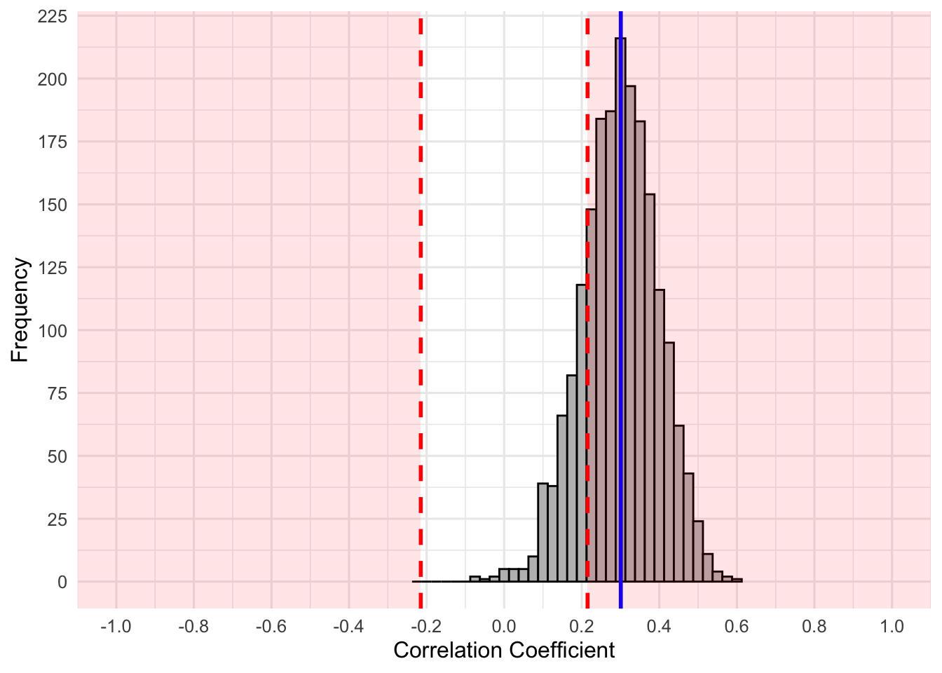
This graph represents the distribution of correlation coefficients for each of our random samples, which were drawn from the 100,000 high schoolers. Notice how they form a seemingly normal distribution around our true population correlation coefficient, $ρ = .300$ . Although it may seem normal, it is actually skewed because of the bounds of the correlation (i.e., -1 to 1). The red lines and shaded regions represent correlation coefficients that are beyond the r = .215 cut-off, which would result in $p < .05$ . Thus, these are statistically significant results in our test of the null hypothesis (i.e., $ρ = 0$ ). The blue line represents the true population correlation coefficient ( $ρ = .300$ ). Just how many samples scored at or beyond the critical correlation value of $r = .215$ ?

The results of our correlations suggest that 1610 correlation coefficients were at or beyond the critical value. Do you have any guess what proportion of the total samples that was? Recall that power is the probability that any study will have $p < α$ . Approximately eighty percent (80.5%) of these studies met that criteria: this was our power! Why is it 80.5 and not 80% exactly? Remember, power refers to a hypothetically infinite number of samples drawn from the population, for any given sample size, effect size, and $α$ . Had we drawn $\infty$ samples, we would have 80% having $p < α$ . Also, our power analysis suggested a sample size of $n = 84.07$ , which is just impossible.

6.3.1 What if we couldn’t recruit 84 participants?

Perhaps we sampled from one high school in a small Canadian city and could only recruit 32 participants. How do you think this would affect our power? Consider that smaller sample sizes are likely to give less precise estimations of population parameters (i.e., the histogram above may be more spread out). However, this influences our critical correlation coefficient, so the red regions shift outward. This will reduce power. Let’s rerun our simulation with 2000 random samples of $n = 32$ to see how it affects out power.

set.seed(372837)
correlations_32 <- pmap(.l=list(sims=1:2000,
                             ss=rep(32, times=2000)),
                      .f=function(sims, ss){
                        df <- sample_n(tbl=data, size=ss, replace = F)
                        r <- cor.test(df$SU, df$SB)$estimate

                        return(r)
                      })

correlations_32 <- do.call(rbind, correlations_32) %>% 
  as.data.frame()

Next we can plot the resultant correlation coefficients. Note that the critical correlation coefficient value for $n = 32$ is larger than for $n = 84$ . The new critical value is $r = 349$ . The following figure is update for the smaller sample:

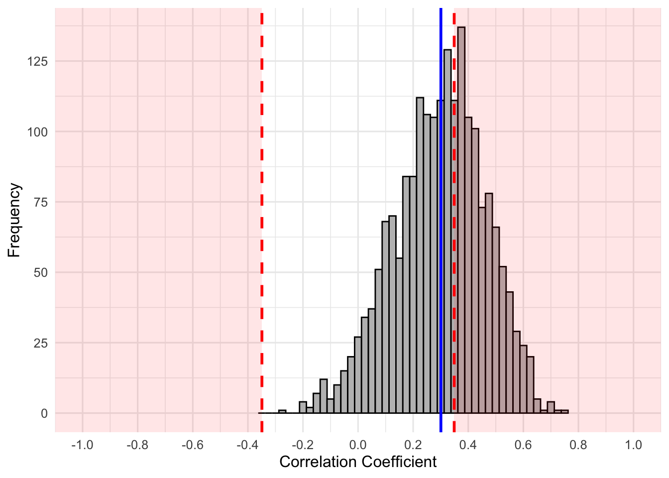
Hopefully, you can see that despite the distribution still centering around the population correlation of $.3$ , the distribution has spread out more. We are less precise in our estimate. Furthermore, the red region (critical r region) is shifted outward due to a smaller $n$ . This would mean that fewer of the samples result in correlation coefficients that fall in the red regions (i.e., power is lower). Would a formal calculation agree? First, let’s find out how many studies resulted in $p < α = .05$ and then do a formal power analysis to determine if they are equal.


   0    1 
1208  792

Our of the 2000 simulated studies, 792 studies yielded statistically significant results ( $792 / 2000 = 39.6 %$ ). Would our power align?

Formal Power Test


     approximate correlation power calculation (arctangh transformation) 

              n = 32
              r = 0.3
      sig.level = 0.05
          power = 0.3932315
    alternative = two.sided

Whoa! Close enough for me. Let’s take it one step further and assume we could only get 20 participants.

Next we can plot the resultant correlation coefficients. Note that the critical correlation coefficient value for $n = 20$ is larger than for $n = 32$ (remember that the null distribution or samples would be spread out more for smaller sample sizes). The new critical value is $r = 444$ . The following is adjusted for 20 participants:

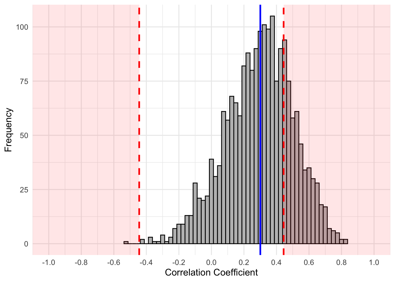
Hopefully, you can see that despite the distribution still centering around our population correlation of .3, the red regions are further outward than the previous two examples. Again, let’s see how many studies resulted in $p < α = .05$ and then do a formal power analysis to determine if they are equal.


   0    1 
1504  496

So, 496 studies yielded statistically significant results ( $496 / 2000 = 24.8 %$ ). Would our power align?


     approximate correlation power calculation (arctangh transformation) 

              n = 20
              r = 0.3
      sig.level = 0.05
          power = 0.2559237
    alternative = two.sided

So, out of 2000 random samples from our population, 24.8% had $p < α = .05$ and our power analysis suggests that 25.6% would. Again, given infinite samples, there would be 25.59237…% with $p < α = .05$ . In sum, as sample size decreases and all other things are held constant, our power decreases. If your sample is too small, you will be unlikely to reject $H_{o}$ even if a true effect exists. Thus, it is important to ensure you have an adequately powered study. More, you may even notice that in the previous figure, a statistically significant result occured in the opposite direction (look in the left red region). Plan ahead. Otherwise, even if a population effect exists, you may not conclude that through NHST’. Or, maybe a non-NHST approach is best ;).

6.4 Increasing Power

Power is the function of three components: sample size, hypothesized effect, $a l p h a$ . Thus, power increases 1. when the hypothesized effect is larger; 2. when you can collect more data (increase $n$ ); 3. or by increasing your alpha level (i.e., making it less strict). This relationship can be seen in the following table:

Population (rho)	Sample Size	Alpha	Power (1-beta)
.1	20	.05	.0670
.1	32	.05	.0845
.1	84	.05	.1482
.1	200	.05	.2919
.3	20	.05	.2559
.3	32	.05	.3932
.3	84	.05	.9776
.3	200	.05	.9917
.6	20	.05	.8306
.6	32	.05	.9657
.6	84	.05	.9999
.6	200	.05	1.000
…	…	…	…
.1	782	.05	.8000
.05	3136	.05	.8000

6.4.1 Effect Size

As the true population effect reduces in magnitude, your power is also reduced, given constant $n$ and $α$ . So, if the population correlation between substance abuse and suicidal behaviors was $ρ = .1$ , we would require approximately $n = 782$ to achieve power of $1 - β = .8$ . In other words, 80% of hypothetically infinite number of samples of $n = 782$ would give statistically significant results, $p < α$ , when $ρ = .1$ . If the population correlation was $ρ = .05$ , we would require approximately $n = 3136$ to achieve the same power. This is the basis of the argument that large enough sample sizes result in statistically significant results, $p < α$ , that are meaningless (from a practical/clinical/real world perspective). If $ρ = .05$ , which is a very small and potentially meaningless effect, large samples will likely detect this effect and result in statistical significance. Hypothetically, 80% of the random samples of $n = 3136$ will result in $p < α = .05$ for a population correlation of $ρ = .05$ . Despite the statistical significance, there isn’t much practical or clinical significance. Statistical significance $\neq$ practical significance.

6.4.2 Estimating Population Effect Size

There are many ways to estimate the population effect size. Here are some common examples in order of recommendation (i.e., try the higher one’s first):

Existing meta-analysis results: some recommend using the lower-bound estimate of presenting CI.
Existing studies that have parameter estimates: some recommend using the lower-bound estimate of the presented CI or halving the effect size of a single study.
Consider the smallest meaningful effect size based on extant theory.
Use general effect size determinations that are considered small, medium, and large. Use the one that makes more sense for your theory.

6.4.3 $α$ level

Recall from above that our alpha level is a criterion that we select to compare our p-values. Reducing our alpha level will result in a larger correlation coefficient criterion that we deem extreme and, thus, smaller red areas. In short, reducing alpha (i.e., more strict criterion) will decrease power, holding all other things constant.

6.5 Power in R

We will focus on two packages for conducting power analysis: pwr and pwr2.

library(pwr)
library(pwr2)

6.5.1 Correlation

Correlation power analysis has four pieces of information. You need any three to calculate the other:

n is the sample size
r is the population effect, $ρ$
sig.level is you alpha level
power is power

So, if we wanted to know the required sample size to achieve a power of .8, with a alpha of .05 and hypothesized population correlation of .25:

## You simply leave out the piece you want to calculate
pwr.r.test(r = .25,
           power = .8,
           sig.level = .05)


     approximate correlation power calculation (arctangh transformation) 

              n = 122.4466
              r = 0.25
      sig.level = 0.05
          power = 0.8
    alternative = two.sided

6.5.2 t-test

With same sized groups we use pwr.t.test. We now need to specify the type as one of ‘two.sample’, ‘one.sample’, or ‘paired’ (repeated measures). You can also specify the alternative hypothesis as ‘two.sided’, ‘less’, or ‘greater’. The function defaults to a two sampled t-test with a two-sided alternative hypothesis. It uses Cohen’s d population effect size estimate (in the following example I estimate population effect to be $d = .3$ :

pwr.t.test(d = .3,
           sig.level = .05,
           power = .8)


     Two-sample t test power calculation 

              n = 175.3847
              d = 0.3
      sig.level = 0.05
          power = 0.8
    alternative = two.sided

NOTE: n is number in *each* group

6.5.3 One way ANOVA

One way requires Cohen’s F effect size, which is kind of like the average Cohen’s d across all conditions. Because it is more common for researchers to use $η_{2}$ , you may have to convert something reported fro another study. You can convert $η_{2}$ to $F$ with the following formula:

Cohen’s F $= \sqrt{\frac{η^{2}}{1 - η^{2}}}$

pwr.1way.test() requires the following:

k = number of groups
f = Cohen’s F
sig.level is alpha, defaults to .05
power is your desired power

pwr.anova.test(k = 3,
               f = .4,
               power = .8,
               sig.level = .05)

6.5.4 Alternatives for Power Calculation

6.5.5 G*Power

You can download here.

6.5.6 Simulations

Simulations can be run for typical designs, which you have seen above through our own simulations to demonstrate the general idea of power. For example, we can repeatedly run a t-test on two groups with a specific effect size at the population level. Knowing that Cohen’s d is:

$d = \frac{{\overset{―}{x}}_{1} - {\overset{―}{x}}_{2}}{s_{p o o l e d}}$

We can use rnorm() to specify two groups where the difference in means is equal to Cohen’s d and when we keep the SD of both groups to 1.

# One time
sample_size <- 20
cohens_d <- .4 ## our hypothesized effect is .4
t.test(rnorm(sample_size), 
       rnorm(sample_size, mean=cohens_d), var.equal = T)


    Two Sample t-test

data:  rnorm(sample_size) and rnorm(sample_size, mean = cohens_d)
t = 0.039978, df = 38, p-value = 0.9683
alternative hypothesis: true difference in means is not equal to 0
95 percent confidence interval:
 -0.6019724  0.6262270
sample estimates:
mean of x mean of y 
0.2923802 0.2802529

We can use various R capabilities to simulate 10,000 simulations and determine the proportion of studies that conclude that $p < α$ .

library(tidyverse)

sample_size <- 20
n_simulations <- 10000
cohens_d <- .4 ## our hypothesized effect is .4
dat_sim <- pmap(.l=list(sims=1:n_simulations),
                .f=function(sims){
                  t.test(rnorm(sample_size), 
       rnorm(sample_size, mean=cohens_d), var.equal = T)$p.value})

## convert to data frame
dat_sim2 <- do.call(rbind, dat_sim) %>% 
  as.data.frame() %>% 
  rename("p"="V1")

This returned a data.frame will 10,000 pvalues from simulations. The results suggest that 2360 samples were statistically significant, indicating 23.6% were statistically significant.

You may be thinking, why do this when I have pwr.t.test? Well, the rationale for more complex designs is the same. For more complicated designs, it can be difficult to determine the best power calculation to use (e.g., imagine a 4x4x4x3 ANOVA or a SEM). Sometimes it makes sense to run a simulation.

Simulation of SEM in R, which can help with power analysis.

Companion shiny app regarding statistical power can be found here.

6.6 Recommended Readings:

Cohen, J. (1994). The Earth is round (p < .05).American Psychologist, 49, 997-1003.
Nickerson, R. S. (2000). Null hypothesis significance testing: A review of an old and continuing controversy. Psychological Methods, 5(2), 241–301. https://doi.org/10.1037/1082-989x.5.2.241
Pritchard, T. R. (2021). Visualizing Power.

6.1 Null Hypothesis Significant Testing

6.2 p-values

6.2.1 If the null hypothesis is true, why would our data be extreme?

6.2.2 Misconceptions

6.2.2.1 Odds against chance fallacy

6.2.2.2 Odds the alternative is true

6.2.2.3 Small p-values indicate large effects

6.3 Power

6.3.1 What if we couldn’t recruit 84 participants?

6.4 Increasing Power

6.4.1 Effect Size

6.4.2 Estimating Population Effect Size

6.4.3 α level

6.5 Power in R

6.5.1 Correlation

6.5.2 t-test

6.5.3 One way ANOVA

6.5.4 Alternatives for Power Calculation

6.5.5 G*Power

6.5.6 Simulations

6.6 Recommended Readings:

6.4.3 $α$ level