| Observations | 100 |
| Dependent variable | y |
| Type | OLS linear regression |
| F(1,98) | 4.67 |
| R² | 0.05 |
| Adj. R² | 0.04 |
| Est. | 2.5% | 97.5% | t val. | p | |
|---|---|---|---|---|---|
| (Intercept) | 44.75 | 28.38 | 61.12 | 5.42 | 0.00 |
| x | 0.17 | 0.01 | 0.33 | 2.16 | 0.03 |
| Standard errors: OLS |
Mediation is a commonly implemented analysis. You already have a wonderful background that can easily be applied to mediation analysis. Mediation is related to the work we have done before, largely linked to \(sr^2\)
Quite simply, we are seeking to understand whether the association between two variables is mediated by a third variable. That is, is the association between \(x_1\) and \(y\) THROUGH \(x_2\). We can visualize this as:
Much mediation research seeks to answer questions – or at least makes it seem like it’s answer– research questions about causality. That is, one thing causes changes in another thing, which causes changes in a third thing. However, regarding causality, running a mediation analysis is no different than running a multiple regression. Causality requires the appropriate research design.
Despite this, mediation is useful for explain mechanisms of association - the why things seem to be related. We will use the famous (maybe infamous) steps by Baron and Kenny (1986), which are often used (and often misinterpreted).
We will focus on basic mediation where there is:
We believe that x is related to y THROUGH m
There are three major steps to our mediation approach.
Is the predictor associated with the criterion?
We first run a regression model with y regressed on x
| Observations | 100 |
| Dependent variable | y |
| Type | OLS linear regression |
| F(1,98) | 4.67 |
| R² | 0.05 |
| Adj. R² | 0.04 |
| Est. | 2.5% | 97.5% | t val. | p | |
|---|---|---|---|---|---|
| (Intercept) | 44.75 | 28.38 | 61.12 | 5.42 | 0.00 |
| x | 0.17 | 0.01 | 0.33 | 2.16 | 0.03 |
| Standard errors: OLS |
This tells use that x is a statistically significant predictor of y. This is analogous to simple regression.
Is the predictor associated with the mediator?
Second, we run a new regression model with m regressed on x:
| Observations | 100 |
| Dependent variable | m |
| Type | OLS linear regression |
| F(1,98) | 22.04 |
| R² | 0.18 |
| Adj. R² | 0.18 |
| Est. | 2.5% | 97.5% | t val. | p | |
|---|---|---|---|---|---|
| (Intercept) | 31.44 | 14.83 | 48.05 | 3.76 | 0.00 |
| x | 0.38 | 0.22 | 0.55 | 4.70 | 0.00 |
| Standard errors: OLS |
This tells use that x is a statistically significant predictor of m. This is also analogous to simple regression.
Is the predictor (x) still associated with the criterion (y) after the mediator (m) is included in the model?
Our last step is slightly more complicated. We will run a regression model with:
\(y\sim x + m\)
\(y_i=b_o+b_3(x)+b_4(m)+e\)
Please note the coefficients above are different from steps 1 and 2 because they will be different when all three variables are in the model.
| Observations | 100 |
| Dependent variable | y |
| Type | OLS linear regression |
| F(2,97) | 15.83 |
| R² | 0.25 |
| Adj. R² | 0.23 |
| Est. | 2.5% | 97.5% | t val. | p | |
|---|---|---|---|---|---|
| (Intercept) | 30.55 | 14.90 | 46.19 | 3.87 | 0.00 |
| x | 0.00 | -0.16 | 0.16 | 0.01 | 0.99 |
| m | 0.45 | 0.28 | 0.63 | 5.08 | 0.00 |
| Standard errors: OLS |
So, what does this tell us? Although in step 1 x was a statistically significant predictor or y, it is no longer when m is included in the model. And since x predicts m, and m predicts y, it would seem that any association between x and y is through m. Please note that I have not used causal language.
A basic mediation (as we have done) figure typically included a few different subscripts. It will typically look like:

In this figure:
We conducted a mediation analysis to determine the extent to which the association between x and y is mediated by m (see Figure 1). Means, SD, and correlations between variables are presented in Table 1.
Table 1

Means, standard deviations, and correlations with confidence intervals


  Variable M      SD    1          2
  1. x     101.36 13.78

  2. m     70.38  12.36 .43**
                        [.25, .58]

  3. y     62.42  11.27 .21*       .50**
                        [.02, .39] [.33, .63]


Note. M and SD are used to represent mean and standard deviation, respectively.
Values in square brackets indicate the 95% confidence interval.
The confidence interval is a plausible range of population correlations
that could have caused the sample correlation (Cumming, 2014).
 * indicates p < .05. ** indicates p < .01.
We used Baron and Kenny’s recommended steps to determine a potential mediation. In step 1, we used x as a predictor of y. Here, x was a statistically significant predictor of y, \(b=.17, p=.003, sr^2=.045, 95\%CI[.00, .015]\). Thus, x accounted for 4.5% of the unique variance in y.
Second, we ran a separate regression model to determine if x was a suitable predictor of m. The results suggest that x is a statistically significant predictor of m, \(b=.38, p<.001, sr^2=.18, 95\%CI[.06, .31]\).
Third, and subsequently, we ran a second block on our first regression model, adding m as a predictor of y. The results indicate that m was a statistically significant predictor of y, \(b=.45, p<.001, sr^2=.20, 95\%CI[.06, .34]\). Importantly, x was no longer a significant predictor of y after m was included in the model, \(b<.00, p=.99, sr^2=.00, 95\%CI[-.00, .00]\). The full model of x and m predicting y accounted for 24.6% of the variance in y, \(R^2=.246\). Thus, m appears to fully mediate the association between x and y (see Figure 1 and Table 2).
Figure 1
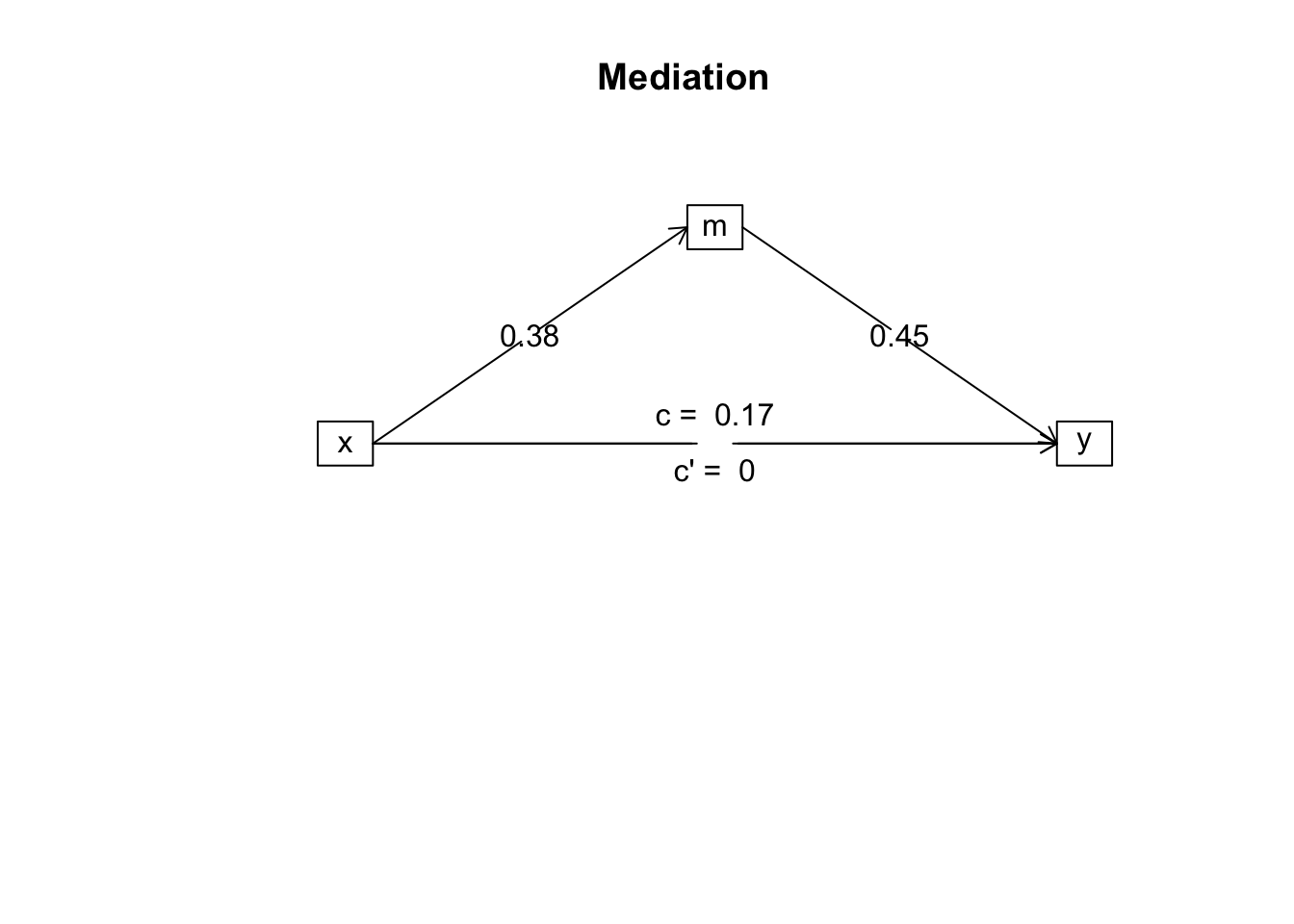
Table 2

Regression results using y as the criterion


   Predictor       b       b_95%_CI beta   beta_95%_CI sr2  sr2_95%_CI     r
 (Intercept) 44.75** [28.38, 61.12]
           x   0.17*   [0.01, 0.33] 0.21  [0.02, 0.41] .05  [.00, .15]  .21*


 (Intercept) 30.55** [14.90, 46.19]
           x    0.00  [-0.16, 0.16] 0.00 [-0.19, 0.19] .00 [-.00, .00]  .21*
           m  0.45**   [0.28, 0.63] 0.50  [0.30, 0.69] .20  [.06, .34] .50**


             Fit        Difference


      R2 = .045*
 95% CI[.00,.15]


     R2 = .246** Delta R2 = .201**
 95% CI[.10,.37]  95% CI[.06, .34]


Note. A significant b-weight indicates the beta-weight and semi-partial correlation are also significant.
b represents unstandardized regression weights. beta indicates the standardized regression weights.
sr2 represents the semi-partial correlation squared. r represents the zero-order correlation.
Square brackets are used to enclose the lower and upper limits of a confidence interval.
* indicates p < .05. ** indicates p < .01.
The following flowchart may also help you in your mediation analysis.
