| ID | Age 4 | Age 6 | Age 8 |
|---|---|---|---|
| 1 | 3 | 5 | 7 |
| 2 | 4 | 3 | 8 |
| 3 | 3 | 5 | 5 |
| 4 | 3 | 3 | 8 |
| 5 | 4 | 4 | 7 |
| 6 | 4 | 4 | 9 |
| 7 | 1 | 4 | 7 |
| 8 | 2 | 3 | 8 |
10 Repeated Measures ANOVA
In progress. Check back soon.
10.1 Our Data
You are hired by the Reach Out Center for Kids (ROCK) as a developmental researcher as part of their cognitive development team. You are tasked with conducting research investigating the changes in memory processes across early childhood. Specifically, you believe that the amount of ‘chunks’ of memory a child can retain increases as children grow. You decide to develop a memory test to assess any changes over time. The test scores range from 0-10 (higher scores indicating better memory). As such, you hypothesize that children’s scores on the test will improve as they grow over time. You recruit eight 4-year olds and follow them over 4 years. You re-assess their memory every two years (i.e., age 4, 6, and 8).
You obtain the following data:
10.2 Our Model
In previous examples of ANOVA, we have had different individuals for each level or condition. Recall that in the one way ANOVA example, each individual received one type of therapy. However, sometimes it makes sense to put the same individuals in each condition to assess change or differences within the individuals. Repeated measures do just that.
As such, our model will look similar:
\(memory = age + error\)
and for each individual:
\(y_i=age_i+e_i\)
10.3 Assumptions
Importantly, one of the major assumptions of the ANOVA is that the observations or independent. This is automatically violated in repeated measures. Despite repeated measures being a strength because it helps us attribute changes to experimental conditions, it is a violation of the assumptions under which our F test was based.
10.3.1 Sphericity
To allows us to continue with F-tests, we must introduce an additional assumption: sphericity and compound symmetry. In short, this assumption purports that the variance of the differences between all conditions is the same and covariances between individuals between conditions is also similar.
An easy way to visualize this is by plotting difference scores. In our example, we will have three difference scores (i.e., age 4 - age 6; age 6 - age 8; age 4 - age 8).
| ID | Age 4 | Age 6 | Age 8 | 4 - 6 | 6 - 8 | 4 - 8 |
|---|---|---|---|---|---|---|
| 1 | 3 | 5 | 7 | -2 | -2 | -4 |
| 2 | 4 | 3 | 8 | 1 | -5 | -4 |
| 3 | 3 | 5 | 5 | -2 | 0 | -2 |
| 4 | 3 | 3 | 8 | 0 | -5 | -5 |
| 5 | 4 | 4 | 7 | 0 | -3 | -3 |
| 6 | 4 | 4 | 9 | 0 | -5 | -5 |
| 7 | 1 | 4 | 7 | -3 | -3 | -6 |
| 8 | 2 | 3 | 8 | -1 | -5 | -6 |
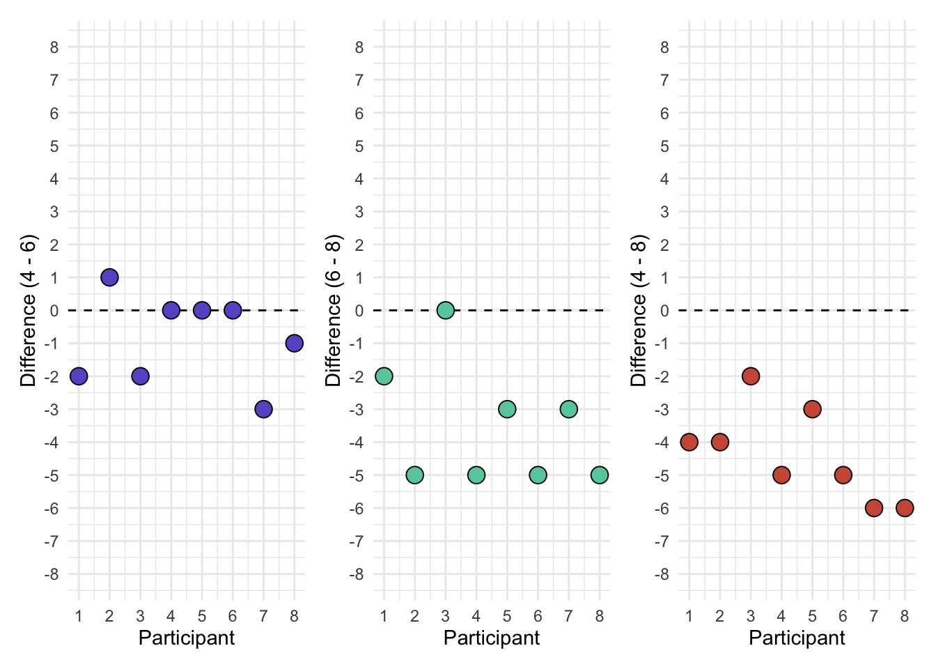
In the visualization we want to look at the dispersion along the y-axis. It should appear similar across the group differences. The variance of each of the differences is:
- Four - Six: 1.839
- Six - Eight: 3.429
- Four - Eight: 1.982
We can test the assumption using Mauchly’s test of Sphericity, which hypothesizes (for a three condition repeated measures deign):
\(H0: \sigma^2_{A-B}=\sigma^2_{A-C}=\sigma^2_{B-C}\)
\(H1:\) var not all equal.
We will not be concerned with the formal calculations of Mauchly’s test; rather, our statistical software can conduct it for us.
For our data:
  Effect         W         p p<.05
2    Age 0.8235094 0.5584776
Recall that the null hypothesis is that the variances are equal; thus, we want p>.05 for Mauchly’s test, although it’s not a complete deal-breaker if we violate this assumptions.
Regardless, our results indicate that we have not violated this assumption and can proceed as intended.
Our data:
We used Mauchly’s test to check the assumption of sphericity and the results indicate that the assumption is not violated, \(p = .558\).
What if I violate the assumption
You can apply two corrections to the data that account for violations of sphericity. These are the Greenhouse-Geisser or Huynh-Feldt corrections.
10.4 Our Analysis
As we have done in the last two chapters, we will partition the various into various subcomponents to determine the appropriate F statistic. The following holds:
You may recall that for independent ANOVAs the individuals in each condition were different. For repeated measures, the individuals will cut across all conditions. So why would they score differently on the same dependent variable? From the figure above, some of the differences may be due to the experiment, while others are just error. It may be helpful to re-conceptualize how we consider variance as the variance between and the variance within an individual. Because all people are in all conditions, changes within an individual can be attributed to the experimental condition and some error.
Let’s calculate some of these and it may help them make sense.
10.4.1 SST
Our total sum of squares is no different than a one way ANOVA.
\(SST=\sum_{i=1}^n(x_i-\overline{x}_{grand})^2\) with \(N-1\) degrees of freedom.
Also, if you know the variance, it can be calculated as:
\(SST=s_{overall}^2(N-1)\)
Our variance in all scores is 4.717 with \(n=24\). Thus:
\(SST=4.717(24-1)=108.49\)
10.4.2 SSW
Here we will depart from our independent ANOVA method. We will calculate the SSW by looking at the deviations within individuals (rather than within groups, which was error in the independent ANOVAs). Recall our data:
| ID | Age 4 | Age 6 | Age 8 |
|---|---|---|---|
| 1 | 3 | 5 | 7 |
| 2 | 4 | 3 | 8 |
| 3 | 3 | 5 | 5 |
| 4 | 3 | 3 | 8 |
| 5 | 4 | 4 | 7 |
| 6 | 4 | 4 | 9 |
| 7 | 1 | 4 | 7 |
| 8 | 2 | 3 | 8 |
So, let’s consider individual \(1\). Their mean score is \(\frac{3+5+7}{3}=5\). And their deviations are:
\(SS_{x_{i=1}}=(3-5)^2+(5-5)^2+(7-5)^2=8\)
We do this across all individuals! The resulting formula is expressed as:
\(SSW=\sum_{i=1,t=1}^n(x_{it}-\overline{x}_{i})^2\)
where \(x_{it}\) is the score for individual \(i\) at time \(t\) and \(\overline{x}_{i}\) is the mean for individual \(i\) across all conditions. If you can quickly get the variances, you could also use the formula:
\(SSW=\sum_{i=1}^ns_{i}^2({n_{t}-1)}\)
For us, we have:
| ID | Variance |
|---|---|
| 1 | 4.000000 |
| 2 | 7.000000 |
| 3 | 1.333333 |
| 4 | 8.333333 |
| 5 | 3.000000 |
| 6 | 8.333333 |
| 7 | 9.000000 |
| 8 | 10.333333 |
and thus, because each individual has three time points:
\(SSW=4(2)+7(2)+1.33(2)+8.33(2)+3(2)+8.33(2)+9(2)+10.33(2)=102.64\)
10.4.3 SSM
The variance of the model, SSM, which is between groups (i.e., experimental conditions) is calculated the same way as before).
\(SSM = \sum_{j=1}^{n_j}{n_j}(\overline{x}_j-\overline{x}_{overall})^2\)
For us, the means are:
| Age | Mean | n |
|---|---|---|
| Mem_4 | 3.000 | 8 |
| Mem_6 | 3.875 | 8 |
| Mem_8 | 7.375 | 8 |
Therefore, because we know our grand mean is 4.75:
\(SSM=8(3.00-4.74)^2+8(3.875-4.74)^2+8(7.375-4.74)^2=85.74\)
10.4.4 SSE
Our error is calculated by removing the SS from the model from within individuals. Remember, individual scores vary because of the experimental conditions (i.e., SSM) and due to error (i.e., random individual fluctuations). Thus, the error can be calculated by subtracting SSM from SSW.
\(SSE=SSW-SSB\)
\(SSE=102.64-85.74=16.90\)
Perhaps now you see an added benefit to repeated measures designs. We have effectively reduced our error term.
10.4.5 Mean Squares
Our mean squares are calculated the same as before. However, our \(df_{e}\) is calculated by \(df_{e}=df_{w}-df_{b}\), where \(df_{w}=n_i(df_{b})\). We have eight individuals with \(df_b=2\), therefore \(df_w=8(2)=16\) and \(df_e=16-2=14\)
\(MSB = \frac{SSB}{df_b}\)
\(MSB = \frac{85.74}{2}=42.87\)
and
\(MSE = \frac{SSE}{df_e}\)
\(MSE = \frac{16.90}{14}=1.207\)
10.4.6 F Statistic
Our F statistic is calculated the same way as before, a ratio of MSB and MSE.
\(F=\frac{MSB}{MSE}=\frac{42.87}{1.207}=35.52\)
We can use an F-distribution table to find out our approximate \(p\)-value. We determine that \(F_{crit}(2, 14)=3.7389\).
However, remember, an ombinus ANOVA does not tell us where the differences are. We have three groups, so we must conduct post-hoc analysis. We looked at this in the one way and factorial ANOVA, so please refer there.
  Tukey multiple comparisons of means
    95% family-wise confidence level

Fit: aov(formula = Memory ~ Age, data = dat_child_long)

$Age
             diff        lwr      upr     p adj
Mem_6-Mem_4 0.875 -0.4367463 2.186746 0.2355710
Mem_8-Mem_4 4.375  3.0632537 5.686746 0.0000001
Mem_8-Mem_6 3.500  2.1882537 4.811746 0.0000034
As you can see, it seems that memory at age eight (\(\overline{x}_{age8}=7.38\), \(SD=1.19\)) is higher than both ages four (\(\overline{x}_{age4}=3.00\), \(SD=1.07\), \(p<.001\)) and six (\(\overline{x}_{age4}=3.88\), \(SD=0.84\), \(p<.001\)). However, memory at age four did not differ than at age six (\(p=.236\)).
10.5 Effect Size
Effect sizes for repeated measures ANOVA are more difficult to calculate by hand. Specifically, we may use generalized eta squared (\(\eta_g^2\)) to account for our repeated measures.
We can get this from statistical software. For this example:
# Effect Size for ANOVA (Type I)

Group  | Parameter | Eta2 (generalized) |       95% CI
------------------------------------------------------
Within |       Age |               0.79 | [0.57, 1.00]

- Observed variables: All
- One-sided CIs: upper bound fixed at [1.00].
Thus, age appears to have a large effect on memory, \(\eta_g^2=.79\), \(95\%CI[.57, 1.00]\).
10.6 Our Results
Recall your hypothesize from above.
you hypothesize that children’s scores on the [memory] test will improve as they grow over time. (You, moments ago).
We conducted an ANOVA to test whether age has an affect on a child’s memory. We used Mauchly’s test to check the assumption of sphericity and the results indicate that the assumption is not violated, \(p = .558\). The results of our omnibus ANOVA suggest that age has a strong and statistically significant effect on a child’s memory, \(F(2, 14)=35.48\), \(\eta_g^2=.79\), \(95\%CI[.63, 1.00]\), \(p<.001\).
Post-hoc results indicated that memory at age eight (\(\overline{x}_{age8}=7.38\), \(SD=1.19\)) is higher than both ages four (\(\overline{x}_{age4}=3.00\), \(SD=1.07\), \(p<.001\)) and six (\(\overline{x}_{age4}=3.88\), \(SD=0.84\), \(p<.001\)). However, memory at age four did not differ than at age six (\(p=.236\)).
10.7 Repeated Measures ANOVA in R
We can use the same ez library to conduct our repeated measures ANOVA in R. Our data will need to be in long format, with each measurement having a row as opposed to each individual. The following data is in long format.
kbl(dat_child_long, caption = "A long dataset.") %>%
kable_styling(full_width = F)| ID | Age | Memory |
|---|---|---|
| 1 | Mem_4 | 3 |
| 1 | Mem_6 | 5 |
| 1 | Mem_8 | 7 |
| 2 | Mem_4 | 4 |
| 2 | Mem_6 | 3 |
| 2 | Mem_8 | 8 |
| 3 | Mem_4 | 3 |
| 3 | Mem_6 | 5 |
| 3 | Mem_8 | 5 |
| 4 | Mem_4 | 3 |
| 4 | Mem_6 | 3 |
| 4 | Mem_8 | 8 |
| 5 | Mem_4 | 4 |
| 5 | Mem_6 | 4 |
| 5 | Mem_8 | 7 |
| 6 | Mem_4 | 4 |
| 6 | Mem_6 | 4 |
| 6 | Mem_8 | 9 |
| 7 | Mem_4 | 1 |
| 7 | Mem_6 | 4 |
| 7 | Mem_8 | 7 |
| 8 | Mem_4 | 2 |
| 8 | Mem_6 | 3 |
| 8 | Mem_8 | 8 |
As you can see, each individual has three rows, one for each time of assessment.
The ezANOVA() function will be used. It will automatically conduct Mauchly’s test because it picks up we have a ‘within’ factor:
ezANOVA(data = dat_child_long, #our data
                 wid = ID, #the ID column;so R knows which rows are the same individuals
                 dv = Memory, #dependent variables
                 within = Age) #independent variable (within)
Warning: Converting "ID" to factor for ANOVA.Warning: Converting "Age" to factor for ANOVA.$ANOVA
Effect DFn DFd F p p<.05 ges
2 Age 2 14 35.48276 3.297595e-06 * 0.7903226
$`Mauchly's Test for Sphericity`
Effect W p p<.05
2 Age 0.8235094 0.5584776
$`Sphericity Corrections`
Effect GGe p[GG] p[GG]<.05 HFe p[HF] p[HF]<.05
2 Age 0.8499856 1.525556e-05 * 1.094312 3.297595e-06 *10.8 Practice Question
You are a educational psychologist testing the efficacy of a new reading program for children who are at-risk for developing a reading disorder. Because assessments are time-consuming, expensive, and with a long waitlist, you are asked to implement a program ASAP and determine it’s efficacy. You develop a program based in the literature and hypothesize a significant improvement in reading ability. You measure reading ability (a measurement that uses t-scores) prior to starting the program, 1 month after being in place, 2 months after being in place (the conclusion of the program), and 3 months (one month after conclusion).
You recruit 6 individual for the program and obtain the following data:
| ID | T0_Month | T1_Month | T2_Month | T3_Month |
|---|---|---|---|---|
| 1 | 38 | 46 | 42 | 42 |
| 2 | 44 | 51 | 52 | 47 |
| 3 | 48 | 53 | 50 | 51 |
| 4 | 39 | 42 | 45 | 35 |
| 5 | 40 | 42 | 41 | 39 |
| 6 | 37 | 42 | 42 | 43 |
Click for the answers.
Warning: Converting "ID" to factor for ANOVA.Warning: Converting "Time" to factor for ANOVA.$ANOVA
Effect DFn DFd F p p<.05 ges
2 Time 3 15 6.656051 0.004470667 * 0.1668966
$`Mauchly's Test for Sphericity`
Effect W p p<.05
2 Time 0.3771464 0.6150885
$`Sphericity Corrections`
Effect GGe p[GG] p[GG]<.05 HFe p[HF] p[HF]<.05
2 Time 0.6226175 0.01702152 * 0.9798512 0.004796211 *Warning: Converting "ID" to factor for ANOVA.
Warning: Converting "Time" to factor for ANOVA.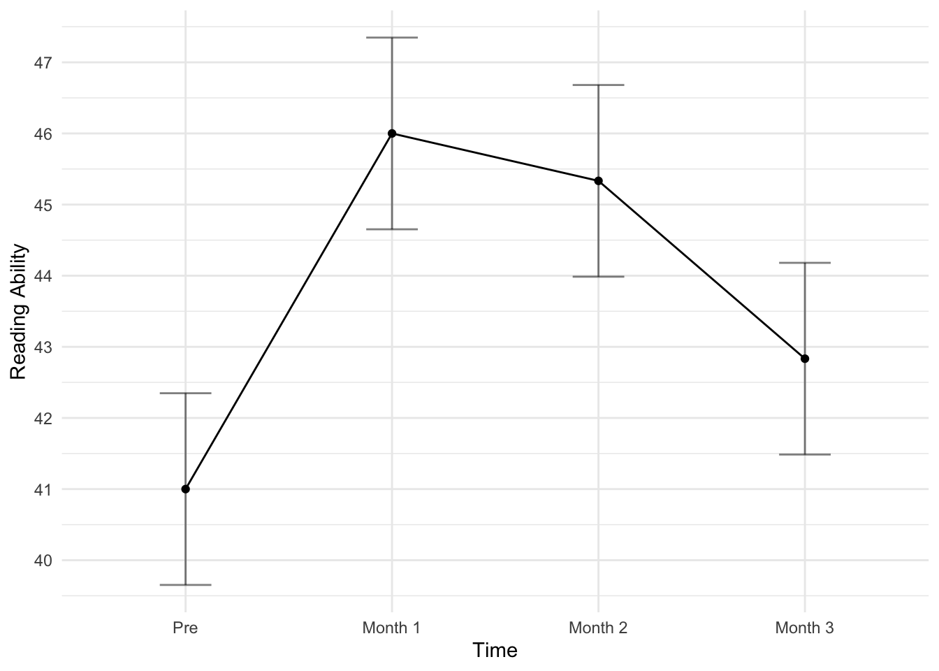
10.9 Additional Readings
- Lakens, D. (2013). Calculating and reporting effect sizes to facilitate cumulative science: A practical primer for T-tests and ANOVAS. Frontiers in Psychology, 4. https://doi.org/10.3389/fpsyg.2013.00863
- Olejnik, S., & Algina, J. (2003). Generalized eta and omega squared statistics: Measures of effect size for some common research designs. Psychological Methods, 8(4), 434–447. https://doi.org/10.1037/1082-989x.8.4.434