| Bag_ID | Flavour | Weight |
|---|---|---|
| 1 | Ketchup | 203.46 |
| 2 | Ketchup | 202.53 |
| 3 | Ketchup | 189.37 |
| 4 | Ketchup | 190.32 |
| 5 | Ketchup | 203.45 |
| 6 | Ketchup | 199.86 |
| 7 | Ketchup | 200.60 |
| 8 | Ketchup | 197.85 |
| 9 | Ketchup | 191.77 |
| 10 | Ketchup | 186.04 |
| 11 | Ketchup | 193.80 |
| 12 | Ketchup | 194.04 |
| 13 | Ketchup | 194.23 |
| 14 | Ketchup | 189.66 |
| 15 | Ketchup | 198.12 |
| 16 | Regular | 206.96 |
| 17 | Regular | 201.44 |
| 18 | Regular | 209.53 |
| 19 | Regular | 195.01 |
| 20 | Regular | 204.16 |
| 21 | Regular | 206.17 |
| 22 | Regular | 198.25 |
| 23 | Regular | 200.89 |
| 24 | Regular | 197.88 |
| 25 | Regular | 198.52 |
| 26 | Regular | 191.28 |
| 27 | Regular | 205.95 |
| 28 | Regular | 191.04 |
| 29 | Regular | 201.97 |
| 30 | Regular | 213.08 |
8 Independent sample t-test
This chapter will cover the t-test, including the distribution, assumptions, hypothesis testing, and equations.
The t-test is used to compare two groups, which is a categorical (independent) variable such as male versus female, time 1 versus time 2, or treatment versus control condition, on some outcome (dependent variable).
In typical experiments, we want to not only randomly sample from the population, but also randomly assign to groups. This procedures allows us to assume that the groups are analogous and that any differences in the outcome are due to the grouping variable. That is, any difference in the DV is attribued to the IV.
If you recall, the null hypothesis typically (and unrealistically) purports that there is no difference/association. Thus, imagine we are comparing two groups: 1 and 2. The null hypothesis states:
\(H0: \mu_1 = \mu_2\)
and the alternative hypothesis states (for a two-sided test)
\(H1: \mu_1 \neq \mu_2\)
In the last chapter we learned about the z-test, which carries a somewhat unrealistic assumptions: that we know some variance-related parameter. Most times we do not know the population standard deviation or variance, so we must estimate using our sample data. Furthermore, in last chapter we simulated the distribution of sample means. We are not longer looking at one mean, but two. We also have two potential standard deviations, but that will come up later.
Let’s use another example similar to the last one. We have a new theory: that Lays purposely puts less chips in a bag of Ketchup Chips than Regular Chips because the seasoning in ketchup chips costs more to produce. From this, we hypothesis that Ketchup Chips (200g) weigh less than Regular Chips (200g). Note that the 200g represents how much the bags supposedly weigh. We annoyingly emailed the company and got the similar response: “All our bags of chips weigh on average 200g, regardless of flavour! Stop email me!”
We decide to purpose two cases of chips (15 bags each) directly from Lays: one Ketchup and one Regular. We get the following data.
And we can summarize the data:
# A tibble: 2 × 5
  Flavour Mean      Min   Max    SD
  <chr>   <chr>   <dbl> <dbl> <dbl>
1 Ketchup 195.673  186.  203.  5.62
2 Regular 201.475  191.  213.  6.36
Let’s visualize the data:
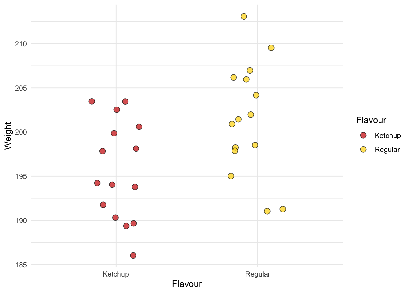
Again, it’s not looking good for lays.
8.1 t distribution
So, if you recall the distribution of sample means, you know that we are going to get some differences in sample means, even if they are drawn from the same population. So, we must somehow make the determination that these two means are different enough to be unlikely if they came from the same distribution.
So, here are the means of our chips from the distribution of sample means:
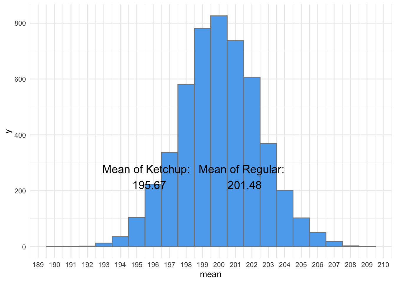
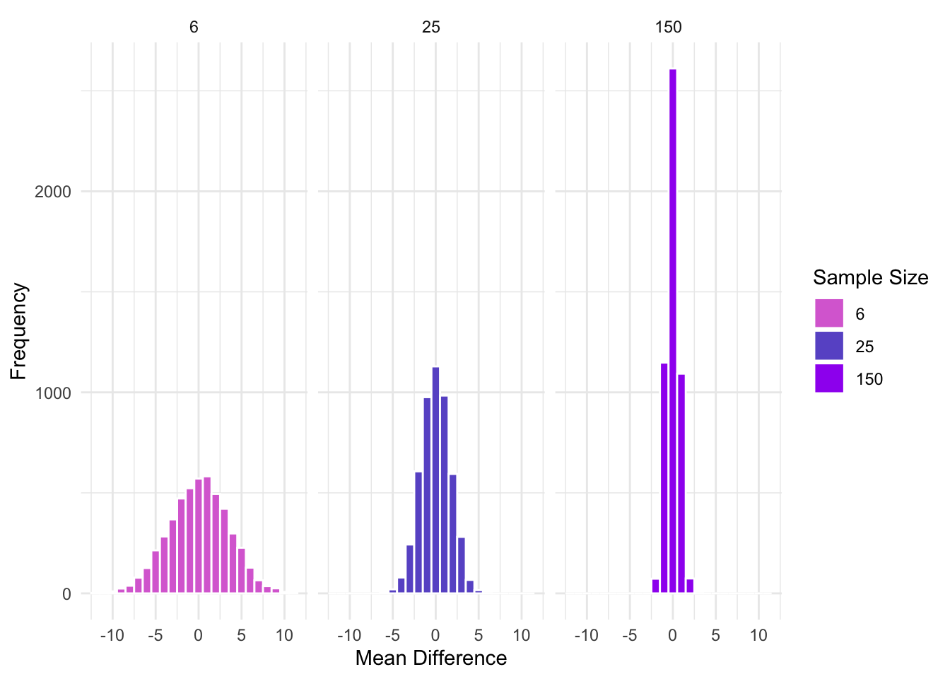
To test our hypothesis, we can build on this distribution. Imagine we subtracted the means of two sample drawn from the distribution above, over, and over, and over. We can model this distribution as well:
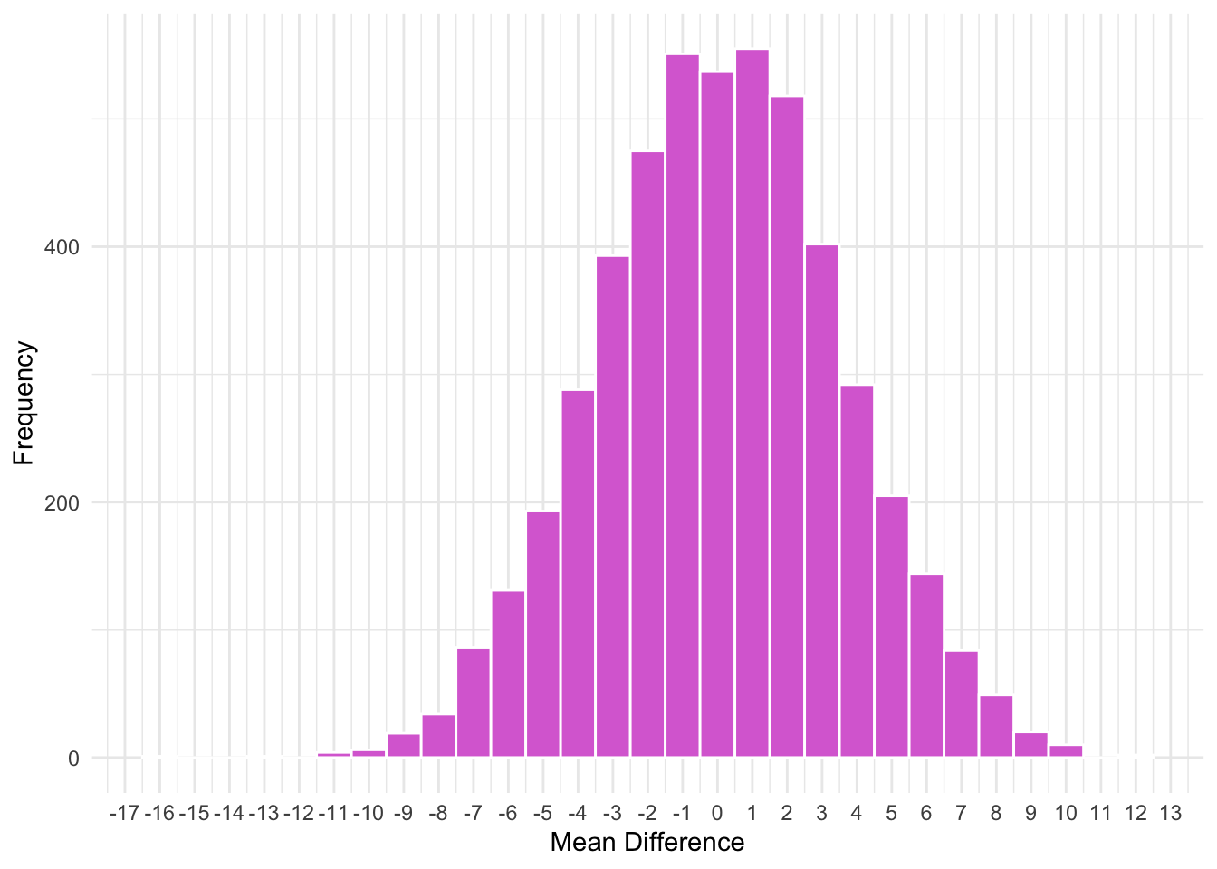
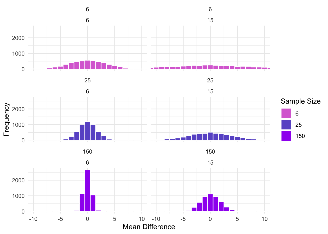
So, when we subtract two means from two sample drawn from the same population, they vary quite a bit. Sometimes one mean is higher, sometimes the other is, and most times they are about the same. However, this will also vary depending on the sample size used for each of the means. For example, let’s compare various sample sizes:
What about when the variance of the samples changes?
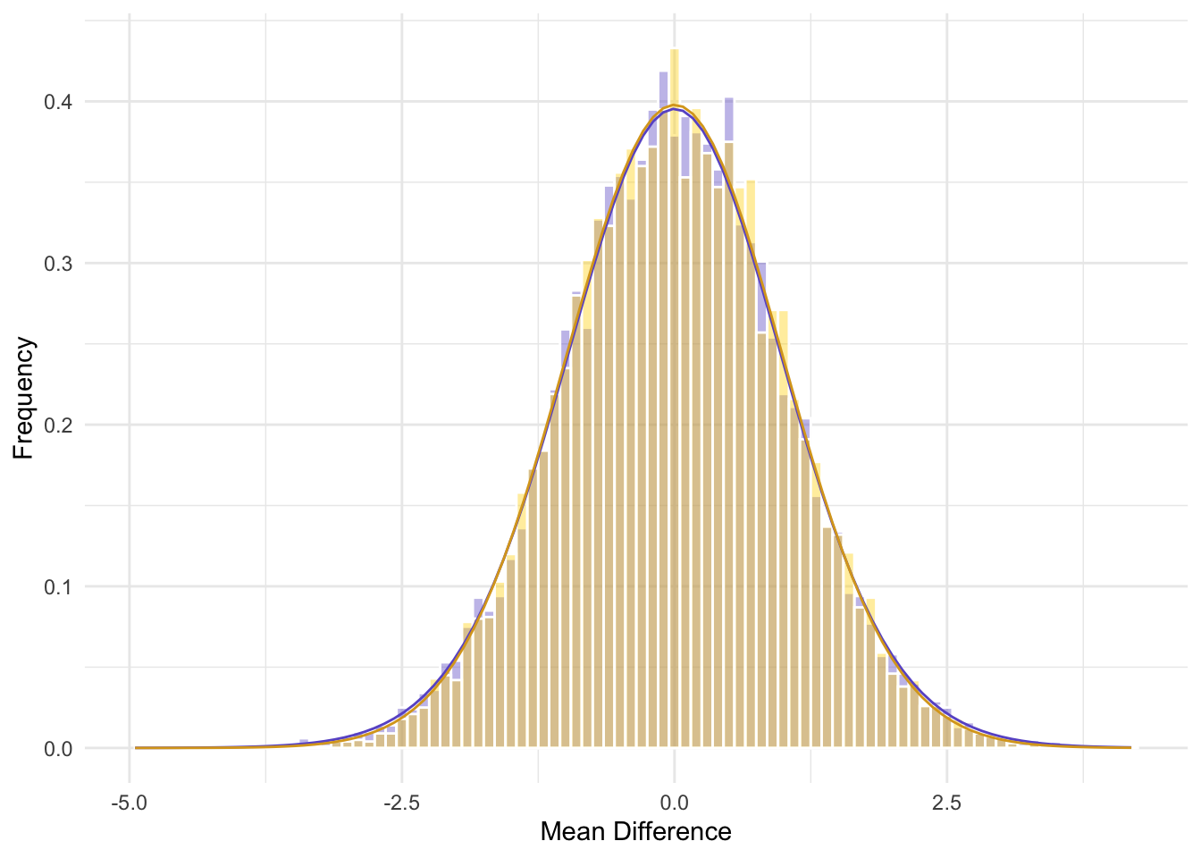
What happens when we divide the mean differences by the standard error of the mean differences? For the t-distribution, the standard error of the mean differences is, for equal sample sizes, \(\sigma_\bar{x} = \frac{\sigma}{\sqrt{n}}\).
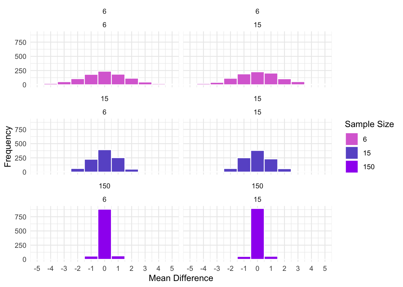
Hopefully, you can see that by dividing by the SE of the mean differences, the distributions are now similar. That is, the differences in the figures based on the difference SD (see above) are not longer present. The above figures represent t-distributions! Using the t distribution, we call determine how likely our sample mean differences if the null hypothesis, that the groups come from the same population with the same mean, is true.
8.2 Assumptions
There are several assumptions we must have when testing from the t distribution.
- First, the data are continuous. For our purposes, this will be interval or ratio data.
- Second, the data are randomly sampled.
- And third, the variance of each group is similar.
8.3 Formulas
The t-test allows you to calculate the t-statistic, which can be compared to the t distribution to determine the probability of the data given the null hypothesis (i.e., p value). The following formulas are relevant.
t-statistic:
\(t = \frac{\bar{x_1} - \bar{x_2}} {\sqrt{\frac{s^2_p}{n_1}+\frac{s^2_p}{n_2}}}\);
where
\(\bar{x_{1}}\) is the mean of group 1;
\(\bar{x_{2}}\) is the mean of group 2;
\(s^2_p = \frac{\Sigma(x_{i1}-\bar{x_1})^2+\Sigma(x_{i2}-\bar{x_2})^2}{n_1+n_2-2}\) is the pooled variance;
and where
\(x_{i1}\) is an individual’s score from group 1; and
\(x_{i2}\) is an individual’s score from group 2.
8.4 Welch’s t-test
There are alternative to Student’s t-test. Specifically, Welch’s t-test is more robust to unequal group variances and smaller sample sizes. Welch’s alters the denominator in the equation to:
\(\sqrt{s^2_{\bar{x1}}+s^2_{\bar{x2}}}\) where
\(s^2_{xi}=\frac{s_i}{\sqrt{n_i}}\)
Furthermore, Welch’s t-test alters the degrees of freedom (v) to:
\(v \approx \frac{\left(\frac{s^2_1}{n_1}+\frac{s^2_2}{n_2}\right)^2}{\frac{s^4_1}{n_1^2v_1}+\frac{s^4_2}{n_2^2v_2}}\)
Importantly, there are no major disadvantages to using Welch’s versus Student’s and you should probably use it in your own research. R’s function t.test() automatically uses Welch’s t-test.
For the purposes of this course, we will use Student’s t-test for our hand calculations. However, you can use Welch’s t-test for any analyses conducted using statistical software.
8.5 Effect Size
Cohen’s d is the standard effect size estimate for a t-test. It is:
\(d=\frac{\overline{x}_1-\overline{x}_2}{s_{pooled}}\)
This is a standardized effect size that be compared across groups of metrics. Cohen suggested the following cut-offs; however, effect size significance is a controversial topic.
- Small - \(d = .2\)
- Medium - \(d = .5\)
- Large - \(d = .8\)
8.6 Ketchup a rip-off?
Let’s go back to our example of ketchup versus regular chips.
We have all the data to calculate our t-statistic.
| Flavour | Mean | Min | Max | SD |
|---|---|---|---|---|
| Ketchup | 195.6733 | 186.04 | 203.46 | 5.615633 |
| Regular | 201.4753 | 191.04 | 213.08 | 6.359418 |
We calculate our squared differences between each bag and the mean of that group, which will be needed later:
| Bag_ID | Flavour | Weight | x_minus_mean_square |
|---|---|---|---|
| 1 | Ketchup | 203.46 | 60.6321778 |
| 2 | Ketchup | 202.53 | 47.0138778 |
| 3 | Ketchup | 189.37 | 39.7320111 |
| 4 | Ketchup | 190.32 | 28.6581778 |
| 5 | Ketchup | 203.45 | 60.4765444 |
| 6 | Ketchup | 199.86 | 17.5281778 |
| 7 | Ketchup | 200.60 | 24.2720444 |
| 8 | Ketchup | 197.85 | 4.7378778 |
| 9 | Ketchup | 191.77 | 15.2360111 |
| 10 | Ketchup | 186.04 | 92.8011111 |
| 11 | Ketchup | 193.80 | 3.5093778 |
| 12 | Ketchup | 194.04 | 2.6677778 |
| 13 | Ketchup | 194.23 | 2.0832111 |
| 14 | Ketchup | 189.66 | 36.1601778 |
| 15 | Ketchup | 198.12 | 5.9861778 |
| 16 | Regular | 206.96 | 30.0815684 |
| 17 | Regular | 201.44 | 0.0012484 |
| 18 | Regular | 209.53 | 64.8776551 |
| 19 | Regular | 195.01 | 41.8005351 |
| 20 | Regular | 204.16 | 7.2074351 |
| 21 | Regular | 206.17 | 22.0398951 |
| 22 | Regular | 198.25 | 10.4027751 |
| 23 | Regular | 200.89 | 0.3426151 |
| 24 | Regular | 197.88 | 12.9264218 |
| 25 | Regular | 198.52 | 8.7339951 |
| 26 | Regular | 191.28 | 103.9448218 |
| 27 | Regular | 205.95 | 20.0226418 |
| 28 | Regular | 191.04 | 108.8961818 |
| 29 | Regular | 201.97 | 0.2446951 |
| 30 | Regular | 213.08 | 134.6682884 |
Let’s fill in the missing data to compute our t-statistic. We have:
\(\bar{x_1} =\) 195.67;
\(\bar{x_2} =\) 201.48;
\(s^2_p = \frac{\Sigma(x_{i1}-\bar{x_1})^2+\Sigma(x_{i2}-\bar{x_2})^2}{n_1+n_2-2} = \frac{441.49+556.19}{15+15-2} = \frac{1007.67}{28} = 35.99\)
and, therefore:
\(t = \frac{195.6733 - 201.4753} {\sqrt{\frac{35.99}{15}+\frac{35.99}{15}}} = \frac{-5.802}{2.190586} = -2.6486\)
We could easily find out the probability of obtaining a t-statistics this low using the distribution:
pt(q=-2.6486, df=28)*2 #We multiple by two because we are using a two-tailed test[1] 0.01313088And a formal t-test should give us the same result:
    Two Sample t-test

data:  Weight by Flavour
t = -2.6487, df = 28, p-value = 0.01313
alternative hypothesis: true difference in means is not equal to 0
95 percent confidence interval:
 -10.289135  -1.314865
sample estimates:
mean in group Ketchup mean in group Regular
             195.6733              201.4753
Thus, the differences in weight between our groups of Ketchup and Regular chips is unlikely given a true null hypothesis, t = -2.65, 95%CI[-10.29, -1.31], p = .013.
8.6.1 Cohen’s D
Recall that:
\(d=\frac{\overline{x}_1-\overline{x}_2}{s_{pooled}}\)
From our above means and pooled variance, we have:
\(d=\frac{195.67-201.48}{\sqrt{35.99}}=-0.968\)
8.6.2 Cohen’s D in R
The effsize package has a function for cohen’s d: cohen.d(). You write your model and specify your data. Essentially the model is “DV ~ IV”. Furthermore, it specifies the CI. For example:
library(effsize)
# our data is called df_chips
cohen.d(Weight ~ Flavour, data = df_chips)
Cohen's d

d estimate: -0.9671509 (large)
95 percent confidence interval:
     lower      upper
-1.7576424 -0.1766594
8.7 Conclusion
From these results, we now have:
| Test | Used for | Hypothesis | Formula |
|---|---|---|---|
| t-test | Testing if two group means are the same | \(H0: \mu_1 = \mu_2\) | \(t = \frac{\bar{x_1} - \bar{x_2}} {\sqrt{\frac{s^2_p}{n_1}+\frac{s^2_p}{n_2}}}\) |
8.8 Practice Questions
Practice Question: Calculate the degree of freedom that would be used in Welch’s t-test on the chip data.
Practice Question: Calculate Student’s t statistics for the following data comparing Sour Cream and Onion (SCO) chips to Salt and Vinegar (SV).
| Bag_ID | Flavour | Weight |
|---|---|---|
| 1 | SCO | 198.3 |
| 2 | SCO | 192.1 |
| 3 | SCO | 204.8 |
| 4 | SCO | 201.6 |
| 5 | SCO | 198.3 |
| 6 | SCO | 196.6 |
| 7 | SV | 193.7 |
| 8 | SV | 197.4 |
| 9 | SV | 199.2 |
| 10 | SV | 198.3 |
| 11 | SV | 213.0 |
| 12 | SV | 205.8 |