15 Multiple Regression
In progress. Check back soon.
Please see here for an additional resource that you may find beneficial: * https://dstanley4.github.io/psyc4780bookdown/multiple-regression.html
15.1 Types of Correlations
15.1.1 \(r\)
We have already explored correlation r in a previous chapter. Recall that when we square the correlation we get the coefficient of determination, indicating the proportion of variance in one variable that is accounted for/explained by (not to be confused with CAUSED BY) the other. Review that chapter is you need to.
15.1.2 \(r_{12.3}\)
15.1.3 \(sr\)
sr is the partial correlation.
15.2 Our data
You are working with Taylor Swift on her new album. She is interested in knowing whether certain characteristics of music are more likely to get played on Spotify. Taylor is specifically interested in the valence (happy to sad) and danceability. You collect a random sample of songs from Spotify and use a computer to estimate the valence and danceability of the songs. These are both measured as continuous variables. You decide to use a regression to determine the effects of both variables, and their interaction, on a song’s popularity (number of plays). All variables are continuous (although regression can handle most variable types; ANOVA is just a special case of regression). Our data is as follows:
| track_artist | track_name | Popularity | Valence | Danceability |
|---|---|---|---|---|
| Camila Cabello | My Oh My (feat. DaBaby) | 208 | 13 | 2 |
| Tyga | Ayy Macarena | 95 | 17 | 7 |
| Maroon 5 | Memories | 200 | 23 | 4 |
| Harry Styles | Adore You | 62 | 9 | 9 |
| Sam Smith | How Do You Sleep? | 189 | 22 | 4 |
| Tones and I | Dance Monkey | 87 | 19 | 7 |
| Lil Uzi Vert | Futsal Shuffle 2020 | 140 | 1 | 5 |
| J Balvin | LA CANCIÓN | 144 | 14 | 5 |
| Billie Eilish | bad guy | 129 | 6 | 7 |
| Dan + Shay | 10,000 Hours (with Justin Bieber) | 141 | 8 | 5 |
| Regard | Ride It | 191 | 13 | 3 |
| Billie Eilish | bad guy | 175 | 19 | 5 |
| The Weeknd | Heartless | 126 | 13 | 4 |
| Y2K | Lalala | 112 | 18 | 5 |
| Future | Life Is Good (feat. Drake) | 36 | 16 | 8 |
| Lewis Capaldi | Someone You Loved | 76 | 17 | 6 |
| Anuel AA | China | 185 | 22 | 4 |
| Regard | Ride It | 162 | 17 | 5 |
| Dua Lipa | Don't Start Now | 144 | 7 | 4 |
| Anuel AA | China | 144 | 12 | 5 |
| Regard | Ride It | 133 | 13 | 5 |
| Bad Bunny | Vete | 107 | 13 | 6 |
| Roddy Ricch | The Box | 142 | 7 | 2 |
| Juice WRLD | Bandit (with YoungBoy Never Broke Again) | 109 | 12 | 7 |
| Roddy Ricch | The Box | 247 | 25 | 4 |
| Regard | Ride It | 133 | 14 | 5 |
| Trevor Daniel | Falling | 149 | 11 | 4 |
| Anuel AA | China | 190 | 15 | 3 |
| Shawn Mendes | Señorita | 140 | 8 | 4 |
| Travis Scott | HIGHEST IN THE ROOM | 186 | 10 | 3 |
| Juice WRLD | Bandit (with YoungBoy Never Broke Again) | 164 | 21 | 4 |
| Camila Cabello | My Oh My (feat. DaBaby) | 135 | 22 | 6 |
| Sam Smith | How Do You Sleep? | 113 | 12 | 5 |
| Harry Styles | Adore You | 129 | 10 | 4 |
| Don Toliver | No Idea | 53 | 20 | 7 |
| Billie Eilish | everything i wanted | 133 | 20 | 5 |
| Lil Uzi Vert | Futsal Shuffle 2020 | 65 | 21 | 7 |
| DaBaby | BOP | 111 | 16 | 5 |
| Lil Uzi Vert | Futsal Shuffle 2020 | 18 | 23 | 8 |
| blackbear | hot girl bummer | 166 | 17 | 4 |
| Tones and I | Dance Monkey | 198 | 13 | 2 |
| Tyga | Ayy Macarena | 87 | 13 | 6 |
| Selena Gomez | Lose You To Love Me | 113 | 11 | 5 |
| Dalex | Hola - Remix | 106 | 15 | 5 |
| The Black Eyed Peas | RITMO (Bad Boys For Life) | 100 | 11 | 8 |
| Arizona Zervas | ROXANNE | 116 | 11 | 6 |
| The Black Eyed Peas | RITMO (Bad Boys For Life) | 111 | 4 | 6 |
| Arizona Zervas | ROXANNE | 101 | 14 | 6 |
| Roddy Ricch | The Box | 57 | 13 | 8 |
| MEDUZA | Lose Control | 119 | 23 | 6 |
15.3 Our (Taylor’s) Hypotheses
In regression you hypothesize about coefficients, typically referred to as \(\beta\)s (beta). For example:
\(H_0:\beta=0\)
\(H_A:\beta\neq0\)
Taylor believes that both both positive and danceable songs will be more popular, but that there will be an interaction between them. Specifically, the more positive, the stronger the relationship between danceability and popularity. We will use two-sided tests for these hypotheses.
15.4 Our Model
Our model can be represented as follows:
\(y_i=\beta_0+x_{1i}\beta_1+x_{2i}\beta_2+x_{1i}x_{2i}\beta_3+e_i\)
Where \(x_{1i}\) is individual \(i\)s score on valence, \(x_{2i}\) is individual \(i\)s score on danceability. \(\beta_0\) is the intercept of the model, \(\beta_1\) is the coefficient for valence, \(\beta_2\) is the coefficient for danceability, and \(\beta_3\) is the coefficient for valence x danceability interaction. \(e_i\) is the error for individual i.
15.5 Our Analysis
15.5.1 A note on ‘centering’
When working in multiple regression, we must consider the multicollinearity of the predictors, which occurs when predictors are highly correlated. When predictors are highly correlated (vague, I know), the standard errors of the \(b\) increase and the estimate is less stable.
Consider how we will interpret a \(b\) coefficient: ‘for 1-unit change in the predictor, we expect a X-unit change in the criterion, holding all other predictors constant.’ But if the predictors are correlated, ‘holding one constant’ seems difficult.
We will talk about diagnosing multicollinearity later, but to be proactive, we can consider centering our predictors. This may have little benefit when not considering interactions, but will be needed when we modelling interactions.
To create an interaction term, we simple multiple the variables we wish to model. We can avoid multicollinearity by first centering these variables. We can subtract each score from the mean of that variable.
Consider our Taylor data:
| track_artist | track_name | Popularity | Valence | Danceability |
|---|---|---|---|---|
| Camila Cabello | My Oh My (feat. DaBaby) | 208 | 13 | 2 |
| Tyga | Ayy Macarena | 95 | 17 | 7 |
| Maroon 5 | Memories | 200 | 23 | 4 |
| Harry Styles | Adore You | 62 | 9 | 9 |
| Sam Smith | How Do You Sleep? | 189 | 22 | 4 |
| Tones and I | Dance Monkey | 87 | 19 | 7 |
To model an interaction, we could create two centered variables for our two predictors (remember, popularity is the criterion). We will need the mean of both valence (\(\overline{x}_{valence}\)=14.48) and danceability (\(\overline{x}_{dance}\)=5.2).
We create a new variable that subtracts each from the mean. The interaction will just be the product of both:
| track_artist | track_name | Popularity | Valence_centered | Danceability_centered | V_D_Interaction |
|---|---|---|---|---|---|
| Camila Cabello | My Oh My (feat. DaBaby) | 208 | -1.48 | -3.2 | 4.736 |
| Tyga | Ayy Macarena | 95 | 2.52 | 1.8 | 4.536 |
| Maroon 5 | Memories | 200 | 8.52 | -1.2 | -10.224 |
| Harry Styles | Adore You | 62 | -5.48 | 3.8 | -20.824 |
| Sam Smith | How Do You Sleep? | 189 | 7.52 | -1.2 | -9.024 |
| Tones and I | Dance Monkey | 87 | 4.52 | 1.8 | 8.136 |
Note that some programs will automatically do this for you; however, you should know why and how it is done.
When we do center our variables, it does change the interpretation of the intercept of the model. Pause here and think about what the intercept represents when the predictors are centered.
We will not use matrix algebra to solve our regression coefficients in this class. However, we could using the following (see here for more information):
\((X^′X)^{−1}X^′Y\)
Where \(X\) is a \(n\) by \(v\) matrix of scores, where n is the number of observations and v is the number of IVs (note: the first column will be 1s to represent the link to the intercept). \(Y\) is a \(n\) by \(1\) vector of scores on the DV.
Here, X is:
And Y is:
\[\begin{bmatrix} 208.00 \\ 95.00 \\ 200.00 \\ 62.00 \\ 189.00 \\ 87.00 \\ 140.00 \\ 144.00 \\ 129.00 \\ 141.00 \\ 191.00 \\ 175.00 \\ 126.00 \\ 112.00 \\ 36.00 \\ 76.00 \\ 185.00 \\ 162.00 \\ 144.00 \\ 144.00 \\ 133.00 \\ 107.00 \\ 142.00 \\ 109.00 \\ 247.00 \\ 133.00 \\ 149.00 \\ 190.00 \\ 140.00 \\ 186.00 \\ 164.00 \\ 135.00 \\ 113.00 \\ 129.00 \\ 53.00 \\ 133.00 \\ 65.00 \\ 111.00 \\ 18.00 \\ 166.00 \\ 198.00 \\ 87.00 \\ 113.00 \\ 106.00 \\ 100.00 \\ 116.00 \\ 111.00 \\ 101.00 \\ 57.00 \\ 119.00 \\ \end{bmatrix}\]The results would work out to:
\[\begin{bmatrix} 75.07 \\ 13.15 \\ 7.54 \\ -2.31 \\ \end{bmatrix}\]Where each row is \(\beta_0\) to \(\beta_3\). Thus, the equation would be:
\(y_i=53.94+x_{1i}(15.18)+x_{2i}(11.50)+x_{1i}x_{2i}(-0.68)+e_i\)
When we had one variable, we could effectively visualize a line of best fit. We can visualize a ‘plane’ of best fit when we have two predictors. When we model the interaction, the plane will have potential curvature. For example, our data is represented as (you should be able to rotate this figure!):
As we now have more variables, the visualization becomes difficult. We struggle to interpret anythign beyond 3D visualization!
15.6 SST
Like simple regression, SST represents the difference between the observed variables and the mean.
\(SST=\sum(y_i-\overline{y})^2\)
15.7 SSR
Like simple regression, SSR represents the difference between the observed variables and the predicted values.
\(SSR=\sum(y_i-\hat{y_i})^2\)
15.8 SSM
Like simple regression, SSM represents the difference between the predicted values and the mean.
\(SSM=\sum(\hat{y_i}-\overline{y})^2\)
Although the main R output does not provide the SS for our model, knowing the above allows you to manually calculate them. For us:
taylors_model2 <- lm(Popularity~Valence_centered*Danceability_centered, data=taylor2)
# Here, my model is 'taylors_model2', which uses the data 'taylor2'
##sse
sse <- round(sum((fitted(taylors_model2) - taylor2$Popularity)^2), 2)
# ssr
ssr <- round(sum((fitted(taylors_model2) - mean(taylor2$Popularity))^2), 2)
#find sst
sst <- round(ssr + sse, 2)

print(paste("SSE = ",sse, ". SSR = ", ssr, ". SST = ",sst,".", sep=""))
[1] "SSE = 16223.73. SSR = 91564.69. SST = 107788.42."Given these, we can calculate the MSR (mean square of the regression; with \(p-1\) degrees of freedom; p being the number of \(b\) coefficients) and MSE (mean square error; with \(n-p\) degrees of freedom) and calculate the appropriate F-statistic.
\(MSR=\frac{91564.69}{3}=30521.56\)
and
\(MSE=\frac{16223.73}{46}=352.69\)
and
\(F=\frac{MSR}{MSE}={30521.56}{352.69}=86.54\)
Given the F-distribution with 3 and 46 degrees of freedom:
x <- seq(0, 10, 1)
ggplot(data.frame(x=x), aes(x))+
  stat_function(fun=df,
                args = list(df1=3,
                              df2=46),
                geom="line")+
  theme_minimal()+
  scale_x_continuous(breaks = seq(0, 100, 1))+
  labs(x="F", y="")+
  theme(axis.text.y = element_blank())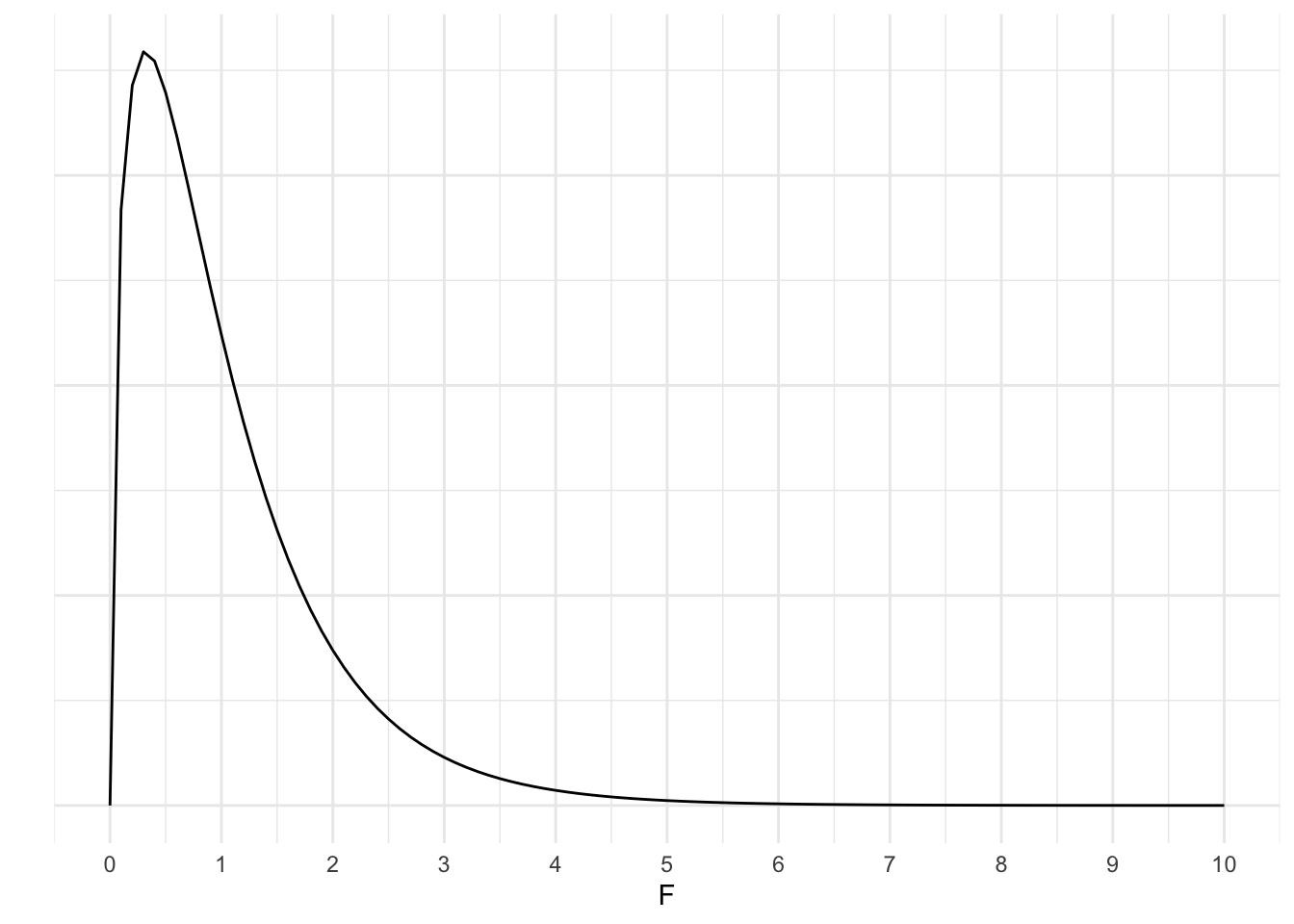
As you can see, our F is extreme in the tail. How extreme?
x <- seq(0, 100, 1)

ggplot(data.frame(x=x), aes(x))+
  stat_function(fun=df,
                args = list(df1=3,
                              df2=46),
                geom="line")+
  theme_minimal()+
  scale_x_continuous(breaks = seq(0, 100, 5))+
  geom_segment(aes(x=86.54, xend=86.54, y=.001, yend=.1))+
  annotate(geom="label", x=75, y=.13, label=paste("Our sample. Less than 0.000001%\n of samples are this or more extreme.", sep=""))+
  labs(x="F", y="")+
  theme(axis.text.y = element_blank())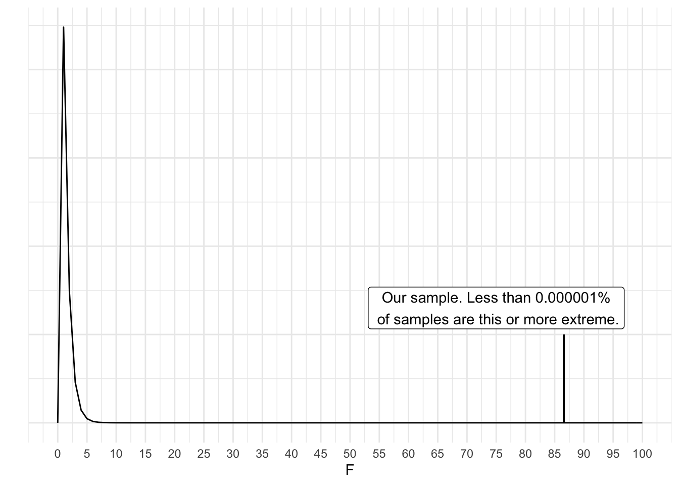
15.8.1 Formal Analysis
There are multiple ways we can run a regression in R. We will use the basic lm() function that we used in the simple regression chapter.
taylors_model <- lm(Popularity ~ Valence_centered +Danceability_centered+V_D_Interaction, data=taylor2)and the summary of that model:
summary(taylors_model)
Call:
lm(formula = Popularity ~ Valence_centered + Danceability_centered +
    V_D_Interaction, data = taylor2)

Residuals:
    Min      1Q  Median      3Q     Max
-32.659 -12.412  -1.021  13.906  43.582

Coefficients:
                      Estimate Std. Error t value Pr(>|t|)
(Intercept)           131.0714     2.6651  49.181  < 2e-16 ***
Valence_centered        1.1600     0.4960   2.339   0.0238 *
Danceability_centered -25.8571     1.6665 -15.516  < 2e-16 ***
V_D_Interaction        -2.3064     0.3332  -6.921  1.2e-08 ***
---
Signif. codes:  0 '***' 0.001 '**' 0.01 '*' 0.05 '.' 0.1 ' ' 1

Residual standard error: 18.78 on 46 degrees of freedom
Multiple R-squared:  0.8495,    Adjusted R-squared:  0.8397
F-statistic: 86.54 on 3 and 46 DF,  p-value: < 2.2e-16
R can calculate the interaction term for us if we specified the model using “*” to indicate the interaction terms, such as:
taylors_model2 <- lm(Popularity~Valence_centered*Danceability_centered, data=taylor2)

summary(taylors_model2)
Call:
lm(formula = Popularity ~ Valence_centered * Danceability_centered,
    data = taylor2)

Residuals:
    Min      1Q  Median      3Q     Max
-32.659 -12.412  -1.021  13.906  43.582

Coefficients:
                                       Estimate Std. Error t value Pr(>|t|)
(Intercept)                            131.0714     2.6651  49.181  < 2e-16 ***
Valence_centered                         1.1600     0.4960   2.339   0.0238 *
Danceability_centered                  -25.8571     1.6665 -15.516  < 2e-16 ***
Valence_centered:Danceability_centered  -2.3064     0.3332  -6.921  1.2e-08 ***
---
Signif. codes:  0 '***' 0.001 '**' 0.01 '*' 0.05 '.' 0.1 ' ' 1

Residual standard error: 18.78 on 46 degrees of freedom
Multiple R-squared:  0.8495,    Adjusted R-squared:  0.8397
F-statistic: 86.54 on 3 and 46 DF,  p-value: < 2.2e-16
Also recall that the apaTables() package provides some additional information that is useful for our interpretation.
library(apaTables)
apa.reg.table(taylors_model)
Regression results using Popularity as the criterion


             Predictor        b         b_95%_CI  beta    beta_95%_CI sr2
           (Intercept) 131.07** [125.71, 136.44]
      Valence_centered    1.16*     [0.16, 2.16]  0.13   [0.02, 0.25] .02
 Danceability_centered -25.86** [-29.21, -22.50] -0.90 [-1.02, -0.79] .79
       V_D_Interaction  -2.31**   [-2.98, -1.64] -0.40 [-0.52, -0.29] .16


  sr2_95%_CI      r             Fit

 [-.01, .05]    .06
  [.65, .93] -.82**
  [.05, .26]   -.24
                        R2 = .849**
                    95% CI[.75,.89]


Note. A significant b-weight indicates the beta-weight and semi-partial correlation are also significant.
b represents unstandardized regression weights. beta indicates the standardized regression weights.
sr2 represents the semi-partial correlation squared. r represents the zero-order correlation.
Square brackets are used to enclose the lower and upper limits of a confidence interval.
* indicates p < .05. ** indicates p < .01.
15.8.2 Measures of Fit
15.9 \(R^2\)
Our effect size is similar to simple regression and represents the proportion of variance the model explains in the outcome. It represents the total contribution of all predictors and is multiple \(R^2\) (multiple given multiple predictors).
\(R^2\) can never go down when we add more predictors. Thus, getting large values for models with lots of variables in unsurprising. However, it does not indicate that any single predictor is doing a good job at uniquely predicting the outcome. More to come on this.
15.10 AIC
Akaike Information Criterion (AIC) is a fit statistic we can use for regression models (and more). The major benefit of AIC is that is penalizes models with many predictors.
\(AIC=n\ln(\frac{SSE}{n})+2k\)
For our above model:
\(AIC=50\ln\frac{16224}{50}+2(4)=297.11\)
Is this good? Bad? Medium? Hard to say. The smaller the number the better. It’s likely easier to interpret several different models from the same data.
15.11 Our Results
More coming soon