| ID | Treatment | OCD_Severity |
|---|---|---|
| 1 | CBT | 12 |
| 2 | CBT | 8 |
| 3 | CBT | 12 |
| 4 | CBT | 10 |
| 5 | CBT | 7 |
| 6 | Rx | 10 |
| 7 | Rx | 10 |
| 8 | Rx | 11 |
| 9 | Rx | 11 |
| 10 | Rx | 14 |
| 11 | CBT_Rx | 9 |
| 12 | CBT_Rx | 6 |
| 13 | CBT_Rx | 8 |
| 14 | CBT_Rx | 9 |
| 15 | CBT_Rx | 8 |
| 16 | Placebo | 12 |
| 17 | Placebo | 14 |
| 18 | Placebo | 15 |
| 19 | Placebo | 12 |
| 20 | Placebo | 17 |
11 One-way ANOVA

Thus far we have compared only two means through our t-tests. Sometimes, we may want to compare more than two groups. ANOVAs allow us to test differences in 2+ groups, and to begin to model multiple IVs influence on a DV.
11.1 Our Data
O’Connor et al. (2006) compared the efficacy of treatments for obsessive compulsive disorder. They measured the severity of OCD symptoms, with lower scores indicating better outcomes (i.e., fewer symptoms). Specifically, they compared differences in OCD severity after individuals received one of:
- Cognitive Behavioral Therapy (CBT)
- Medication
- CBT + Medication
- Placebo
We will use research design to conduct a similar analysis using fake data. Our data are as follows:
Click to expand the data
Theoretically, we could do six t-tests:
- CBT versus Medication
- CBT versus CBT + Medication
- CBT versus Placebo
- Medication versus CBT + Medication
- Medication versus Placebo
- CBT + Medication versus Placebo
However, this would result in an inflated Type I error rate. Recall that we typically set our \(\alpha = .05\). Thus, the rate to not get a Type I error is \(.95\). With six independent comparisons our alpha rate actually becomes:
\(1-(1-\alpha)^{n_{comparisons}}=1-(1-.05)^6 = .265\)
Our Type I error rate would go from 5% to 26.5%! This means that if all these comparisons were statistically significant, at least one is likely a Type I error. An analysis of variance (ANOVA) allows us to compare 2+ groups within a single test – and as you will see later, multiple IVs at once. Specifically, we can test an independent variable’s (with two or more levels) association with a dependent variable. Prior to diving into ANOVAs, I would like to explain the F-distribution, which is at the core of ANOVAs.
11.2 F Distribution
I remember hearing about the F-test during my third year undergraduate statistics class. I enjoyed statistics courses, more so than the average psychology student, at least I believed so. I felt comfortable with the equations to calculate SSE, MSB, and so on, but I never gave much thought about why a certain F value was considered statistically significant. In fact, we were never taught about what p-values mean during my undergrad (2012-2015). Well, if you are an undergrad - or anyone really, I won’t discriminate - you are in luck! I will (hopefully) enlighten you about the F-distribution. Before we dive into the F-distribution, we must better understand the underpinning: the chi-square distribution.
11.2.1 The Chi-square Distribution
Consider an independent and normally distributed variable: IQ. Let us take a random sample of four 20-year-olds and measure their IQ. Perhaps their scores are:
| Name | IQ |
|---|---|
| Alicia | 85 |
| Ramona | 108 |
| Marie | 91 |
| Julianna | 108 |
Given that we know the mean IQ is 100 with a standard deviation of 15, we can standardize this variable by converting them to z-scores. To convert to a z-score, we subtract each score from the mean and divide by the standard deviation: \(z = \frac{x_i-\mu}{SD}\). Thus, our z-scores are:
| Name | IQ | z-score |
|---|---|---|
| Alicia | 85 | -1.00 |
| Ramona | 108 | 0.53 |
| Marie | 91 | -0.60 |
| Julianna | 108 | 0.53 |
So, Alicia has a z-score of -1.0 (i.e., 1 SD below the mean) and Ramona about 0.5 (i.e., about 0.5 SD above the mean). We can also call these z-scores standard deviates. They deviate around the mean in standard distribution. These are also known as independent and identically distributed variables (IID). We can calculate the sum of squares, \(SS = \sum_{i=1}^n(x_n-\mu)^2\) for any given number of observations. That is, we take each score, subtract it from the mean, square it, and add them all up. Because the standardized distribution has a mean of \(0\) and a standard deviation of \(1\), the sum of squares of our sample is, simply, our squared z-scores:
\(SS = \sum_{i=1}^n{z_i^2}\)
here:
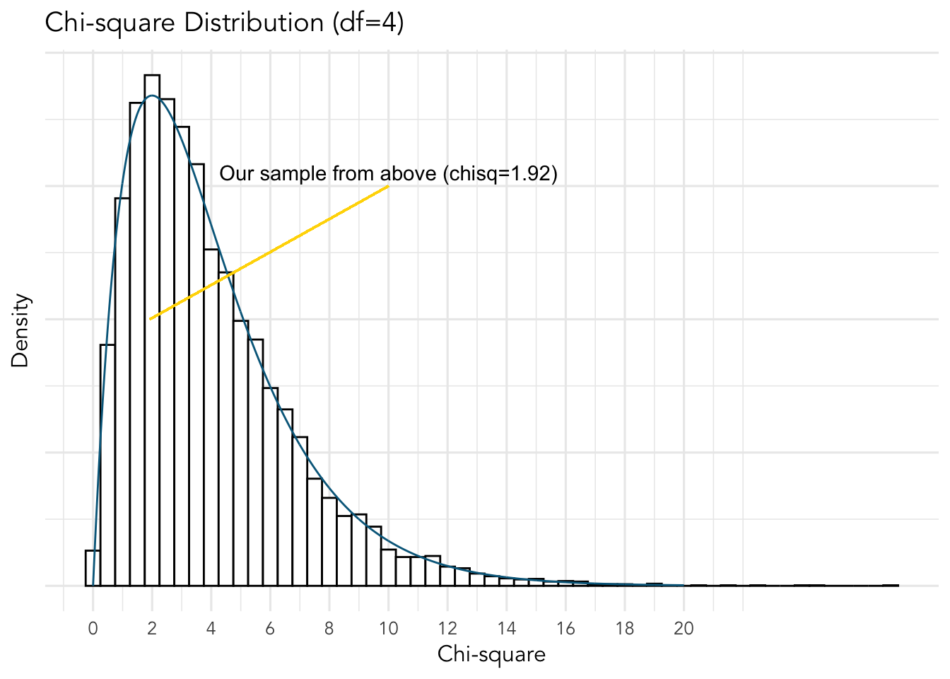
\(SS = (-1)^2+0.53^2+(-0.6)^2+0.53^2 = 1.9218\)
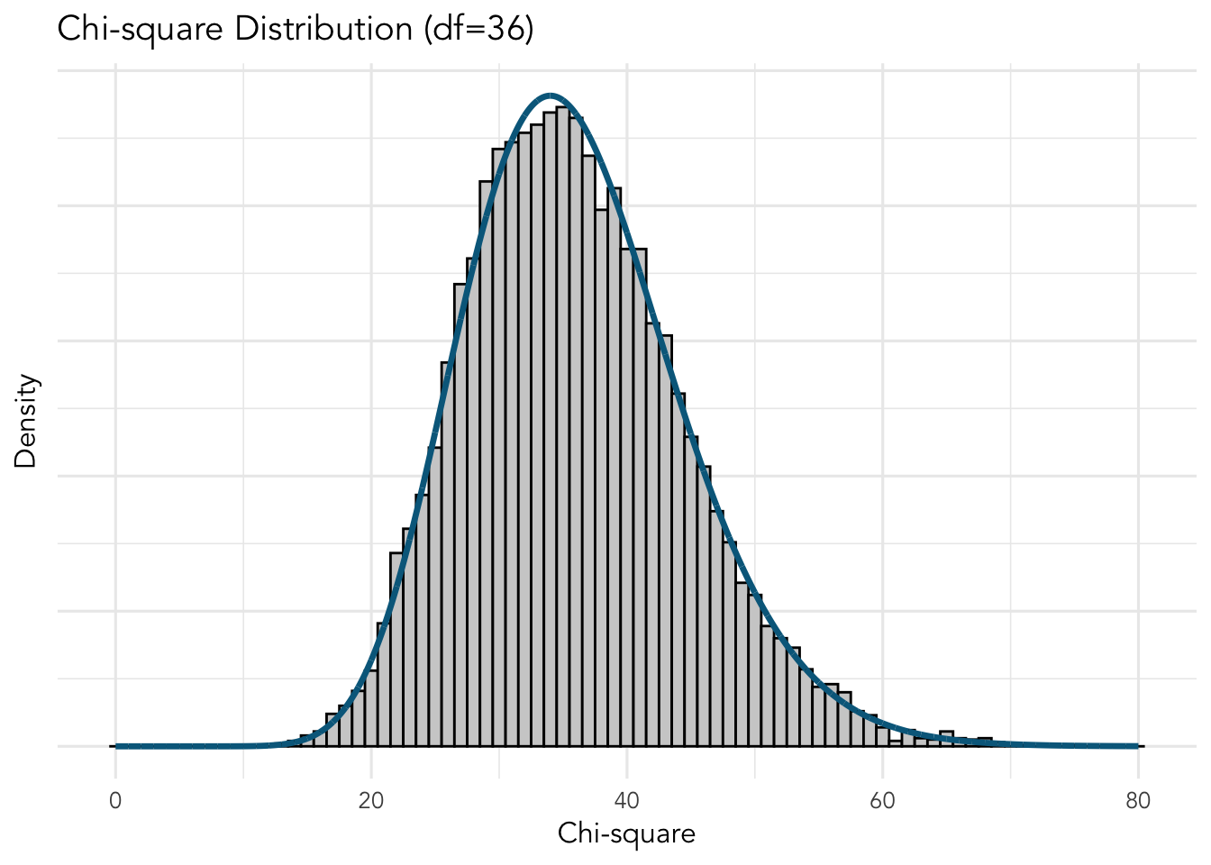
So…why does all this matter? A chi-square value is the sum of squares of standard deviates. The chi-square distribution is the distribution of the sum of squares of a given number of deviates, our df, under repeated (infinite) samples. So, if we randomly sampled four people an infinite number of times, the sum of squared deviates would form a chi-square distribution with four df. Here’s what that would look like”
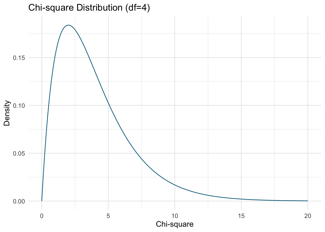
The above is know as a probability density function (PDF). It uses fancy calculus to determine it’s shape. We could also simulate 10,000 random samples of four individuals (using some simple R code). We will calculate the chi-square value for each sample using the sum of their squared standard deviate (i.e., mean of 0 and standard deviation of 1). We will then plot the chi-square values in a histogram; I will overlay the above chi-square PDF over our graph.
The shape of the chi-square distribution depends on one parameter: the number of observations drawn or degrees of freedom (df). The mean of the distribution is equal to its df (i.e., for our above data (the many simulation) the mean is approximately 4. Furthermore, the chi-squared distribution approaches a normal distribution as df increases. Here is the distribution with some other df:
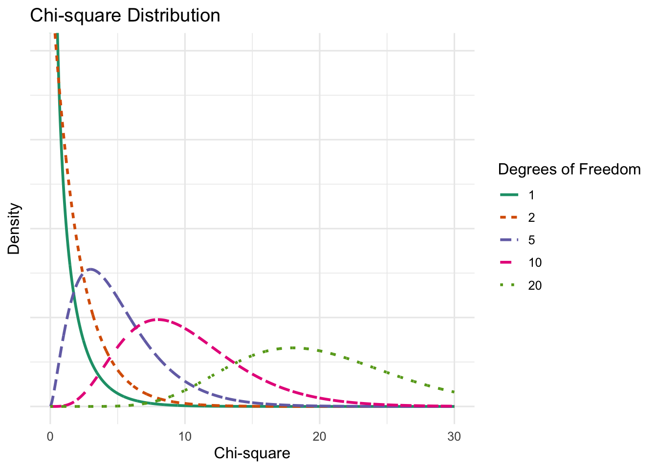
As you can see, the distribution approaches normality as the df increases.
So, recall that the chi-square is the sum of squares deviations (\(SS\)):
\(SS = \sum_{i=1}^n(x_n-\mu)^2\)
We can scale the SS to estimate variance. Recall that variance is the sum of squares divided by number of observations:
\(\sigma^2 = \frac{\sum_{i=1}^n(x_n-\mu)^2}{n}\)
or an unbiased estimate in the sample:
\(s^2 = \frac{\sum_{i=1}^n(x_n-\mu)^2}{n-1}\)
Thus, we can scale the chi-square by dividing by df, which will give us estimate of a variance.
11.3 From Chi to F
The F-distribution is a ratio of two scaled (i.e., divided by their df) chi-square distributions. We can see the similarities between a scaled chi-square:
\(\chi^2 = \frac{\sum_{i=1}^n(z^2)}{n}\)
and the equation for population variance:
\(\sigma^2 = \frac{\sum_{i=1}^n(x_n-\mu)^2}{n}\)
Thus, the F-distribution is approximately the ratio of two variances that some from the same population. If you were to infinitely sample from a population, scale the resulting chi-squares, and get their ratio, you would end up with the F-distribution. What do these variances have to do with ANOVA? Well, ANOVA estimates the ratio of the variance in the means of the IV group(s) (mean squared between; \(MSB\)) to the variance between each individual’s score within a group with that group’s mean (i.e., mean squared error/within; \(MSE/MSW\)). If the groups do not differ (i.e., they are randomly sampled from the sample population), the variances should be approximately equal. Given that they are assumed through the null hypothesis to be from the same population, the resulting F-distribution should be the ratio of chi-squares. An example of an F-distribution with \(df_1=4\) and \(df_2=36\) (i.e., the numerator variance is chi-square with \(df=4\) and the bottom chi-square with \(df=36\)).
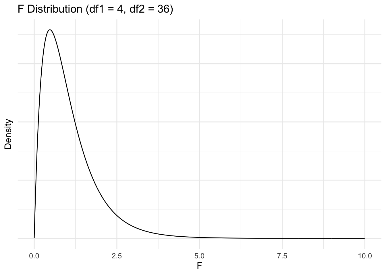
We can recreate this figure. First, we will reuse our extant chi-square distribution that we simulated above (\(df=4\)). Second, we simulate a new chi-square distribution with 36 degrees of freedom. Then, we will divide pairings of each and plot the histogram. Although the actual F-distribution is created using fancy calculus, I will divide 1 of each distribution by 1 of the other. Although this is not an exact estimation, it should be a decent approximation with 10’000 samples each. Here is our simulated chi-square (df=36) distribution:
Let’s combine the data and scale them appropriately by dividing by the number of observations:
\(\frac{\chi^2}{n} = \frac{\sum_{i=1}^n(z^2)}{n}\)
Let’s look at each scaled distribution:
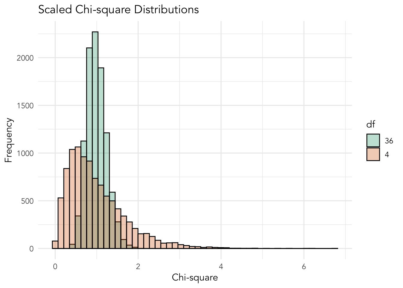
Note how that scaling the chi-square distributions do not create a distribution with \(df=1\).
Let’s divide each 10,000 pairings of the two chi-square distributions to create:
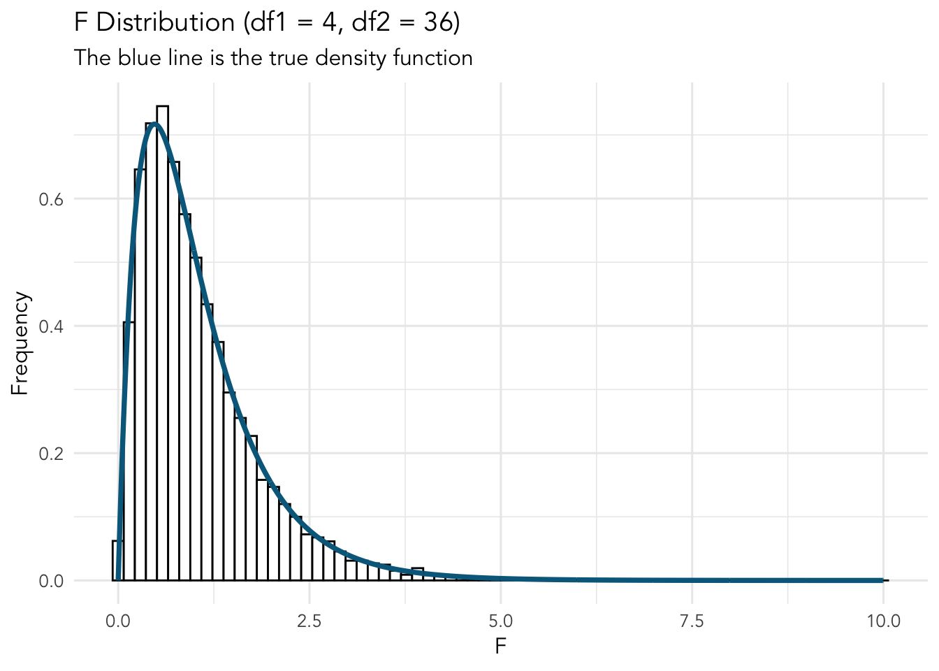
Fantastic. Even with just 10’000 observations, we have approximated the F-distributions density function. Remember, the true distribution would account for an infinite number of ratios of chi-squares of \(df_1=4\) and \(df_2=36\).
11.4 Back to ANOVA Example - OCD Treatment
Above we used z-scores to calculate two scales chi-squares which are used to get an F statistic and compared to the F-distribution. Now, let’s consider the following data, which is based on groups in the study mentioned at the beginning of this chapter, which investigated the efficacy of treatment for OCD.
|
|
11.4.1 Hypothesis
Our most basic null and alternative hypothesis are as follows:
\(H_0: \mu_1=\mu_2=...\mu_n\) (all the means are equal)
\(H_1: \mu_1\neq\mu_2\neq...\mu_n\) (the means are not equal)
This is the general structure of \(H_0\) and \(H_1\) in ANOVA designs.
Furthermore, we way specifically hypothesis that two or more specific group will differ in a specific manner. For example, we may hypothesize that all three treatment groups will have less OCD symptom severity than the placebo group, but that the treatment groups will not differ:
\(H:\mu_{placebo}<\mu_{CBT}=\mu_{Rx}=\mu_{CBT+Rx}\)
Note that this hypothesis would replace \(H_1\) above in this specific study.
We can test these hypotheses through an ANOVA and post-hoc tests.
11.5 Our Model
Using the above hypothesis, we can frame our model as:
\(outcome_i=group+error_i\)
or more specifically, and expanded on below:
\(y_i=\beta_0+x_igroup_i+error_i\)
11.6 Our Analysis
Recall from above when we learned about Chi-square distributions that the standard deviates from above were scores subtracted from the mean (specifically the sum of squared z-scores). We can do the same thing here for two separate components of our data. Essentially, it is the variances of our model (that the groups’ means differ) compared to the variances of the error (each score compared to its group’s mean). Our model will have three total components that we can calculate (we can get by with calculating only two of them), namely, sum of squares total (SST), sum of squares of the model/between groups (SSB), and sum of squares within groups/error (SSE). They are related in the following way:
\(SST = SSB + SSE\)
Descriptions of each follow along with visualizations.
11.6.1 SST
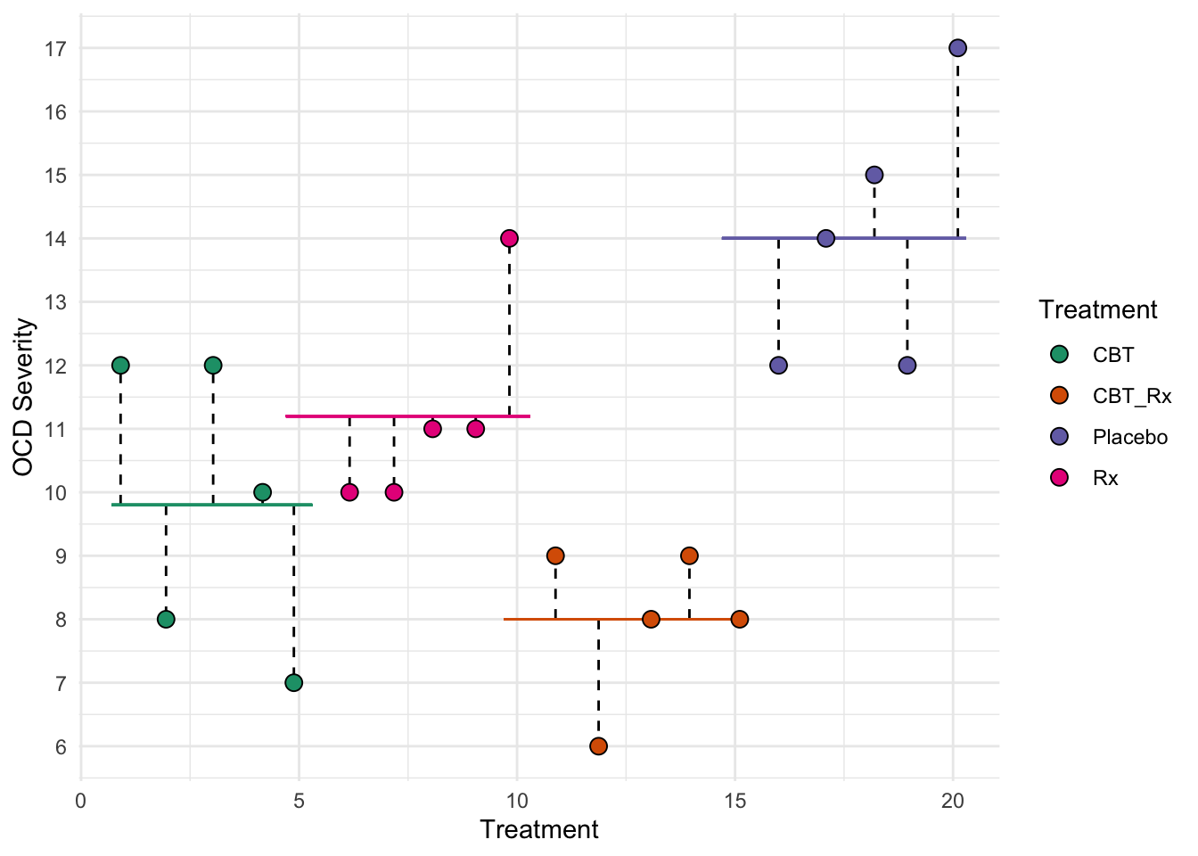
The sum of squares total represents all the deviations of the model. It is each score compared to the overall (grand) mean. Is it represented by:
\(SST = \sum_{i=1}^n(x_i-\overline{x})^2\)
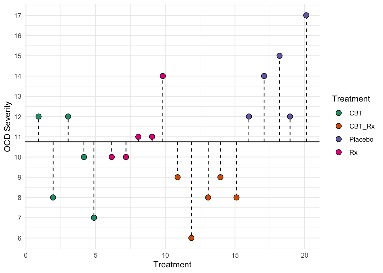
This first figure represents the total deviations used to calculate SST. Each dotted lined represents the difference between each individual and the grand mean (the solid black line). Recall that the grand mean is the mean of all individuals.
11.6.2 SSE
The sum of squares error SSE represents the deviation of each individual from their group mean.
\(SSE = \sum(x_{ij}-\overline{x}_j)^2\)
where \(x_{ij}\) is individual \(i\) in group \(j\) and \(\overline{x}_j\) is the mean of group \(j\). For the above data, for example the CBT group, we can calculate SSE. First, the mean of the CBT group is:
\(\overline{x}_{CBT}=\frac{12+8+12+10+7}{5} = 9.8\)
and, thus:
\(SSE_{CBT}=(12-9.8)^2+(8-9.8)^2+(12-9.8)^2+(10-9.8)^2+(7-9.8)^2 = 55.60\)
We would do this for each group and sum them. This second figure represents SSE. Each dotted lined represents the difference between an individual and their group’s mean. The colored lines represent each groups mean.
You should notice that the length of the dotted lines are smaller than the lengths in the first figure. Thus, the model seems to be doing a good job at explaining our data.
11.6.3 SSB
The sum of squares between groups (SSB) represents the deviation of each group’s mean from the grand mean.
\(SSB = \sum_{j=1}^{n_j}{n_j}(\overline{x}_j-\overline{x}_{overall})^2\)
where \(n_j\) is the sample size for group \(j\); and
\(\overline{x}_{overall}\) is the overall/grand mean.
It can get confusing when different places use different names for these. For example, we called the total sum of squares SST, but some places call the sum of squares between SST (treatments). We will stick to the following for a one way ANOVA:
Sum of squares total (SST)
Sum of squares between groups (SSB)
Sum of squares error (SSE)
SST = SSB + SSE
Our group means are:
| Treatment | Mean |
|---|---|
| CBT | 9.8 |
| CBT_Rx | 8.0 |
| Placebo | 14.0 |
| Rx | 11.2 |
and our overall mean is \(\overline{x}_{overall} = 10.75\). Also, there are five individuals per group. Therefore:
\(SSB = 5(9.8-10.75)^2+5(8.0-10.75)^2+5(14.0-10.75)^2+5(11.2-10.75)^2 = 96.15\)
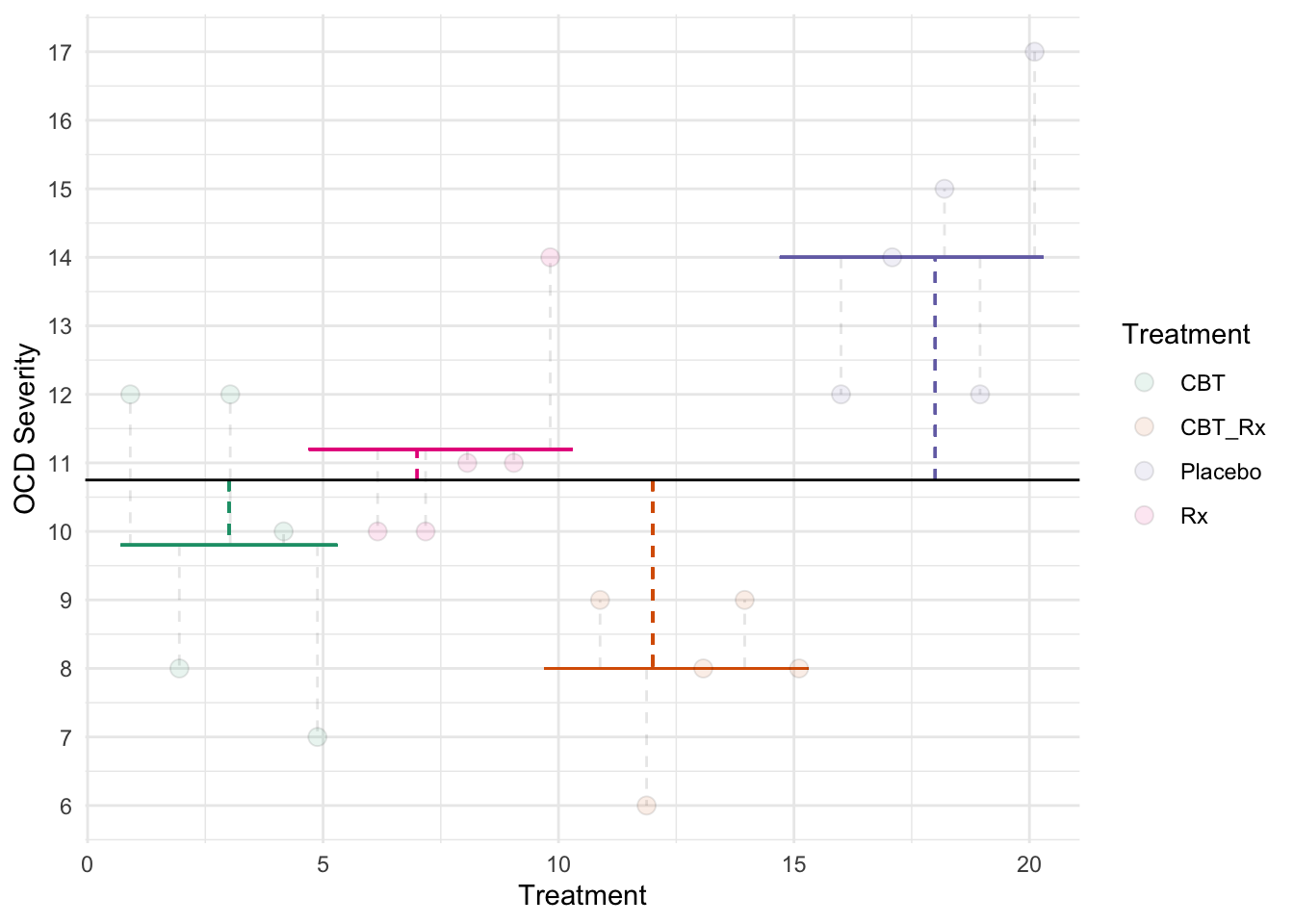
This third figure represents SSB. Each dotted lined represents the difference between a group’s mean and the grand mean. The colored lines represent each groups mean. The black line represents the grand mean.
11.6.4 Mean Squares
We must also scale the sum of squares to become variances by dividing by the degrees of freedom. Our \(df\) are \(df_b=k-1\) (where k is the number of groups) and \(df_e = N-k\). This results in two Mean Squares. These are, essentially, variances.
\(MSB = \frac{SSB}{df_b}\)
and
\(MSE = \frac{SSE}{df_e}\)
If you remember the above regarding the F distribution, you may intuitively relate it to the OCD treatment example, wherein:
\(F = \frac{MSB}{MSE}\)
We can determine how likely or unlikely our data are using the F-distribution of \(df_b\) and \(df_w\) degrees of freedom.
Thus, the above example would results in:
\(MSB = \frac{96.15}{4-1}=32.05\);
\(MSE = \frac{55.6}{20-4}=3.48\); and
\(F=\frac{32.05}{3.48}=9.223\)
We will compare this statistic to the distribution to determine how probable our data are compared to the null hypothesis. If our F is large enough to be unlikely given the null, we would reject it. The F statistic is an omnibus test.
Omnibus Tests
Omnibus tests, or global tests, determine the ratio of variance explained by the model versus error. In our F-test, it tells us that at least two of the means differ, but does not tell us which one. Thus, we need to conduct some form of post-hoc (after the event) tests.
If the omnibus test is not statistically significant, you can stop there. The groups in the IV do not differ.
We can use an F-distribution table to find out our approximate \(p\)-value. The table suggests that critical F for our degrees of freedom is \(F(3, 16)=3.2389\) for an \(\alpha=.05\). Our obtained F is higher (\(F_{obtained} > F_{critical}\); \(9.223>3.239\)). This site can calculate exact p-values. This site returns a p-value of \(p=.00089\).
You can use R to calculate exact p-values as well using the pf() function (probability of F). It requires arguments for your F (q), df1 and df2. Also, be sure to specify that lower.tail=F, indicating you want the probability on the right sid eof the distribution. For example, writing pf(q=9.223, df=3, df2=16, lower.tail=F) returns 8.9002206^{-4} Thus, our data are quite unlikely given a true null hypothesis. We have a statistically significant result.
11.7 Our Results
We conducted a one way ANOVA to determine the association between OCD treatments and OCD severity. The results suggest that the group means for OCD severity are unlikely given a true null hypothesis, \(F(3, 16)=3.24\), \(p<.001\).
11.8 Post-hoc Tests
So our ANOVA revealed a statistically significant results, but it was an omnibus test. Now what? Unfortunately, the results of the omnibus ANOVA test does not inform us which groups differ. It simply tells us at least one group differ from at least one other group.
Recall that our family wise error rate increases as we do more statistical tests. So, while we may have set a criterion of \(\alpha=.5\), it increases as we do more tests.
`geom_smooth()` using method = 'loess' and formula 'y ~ x'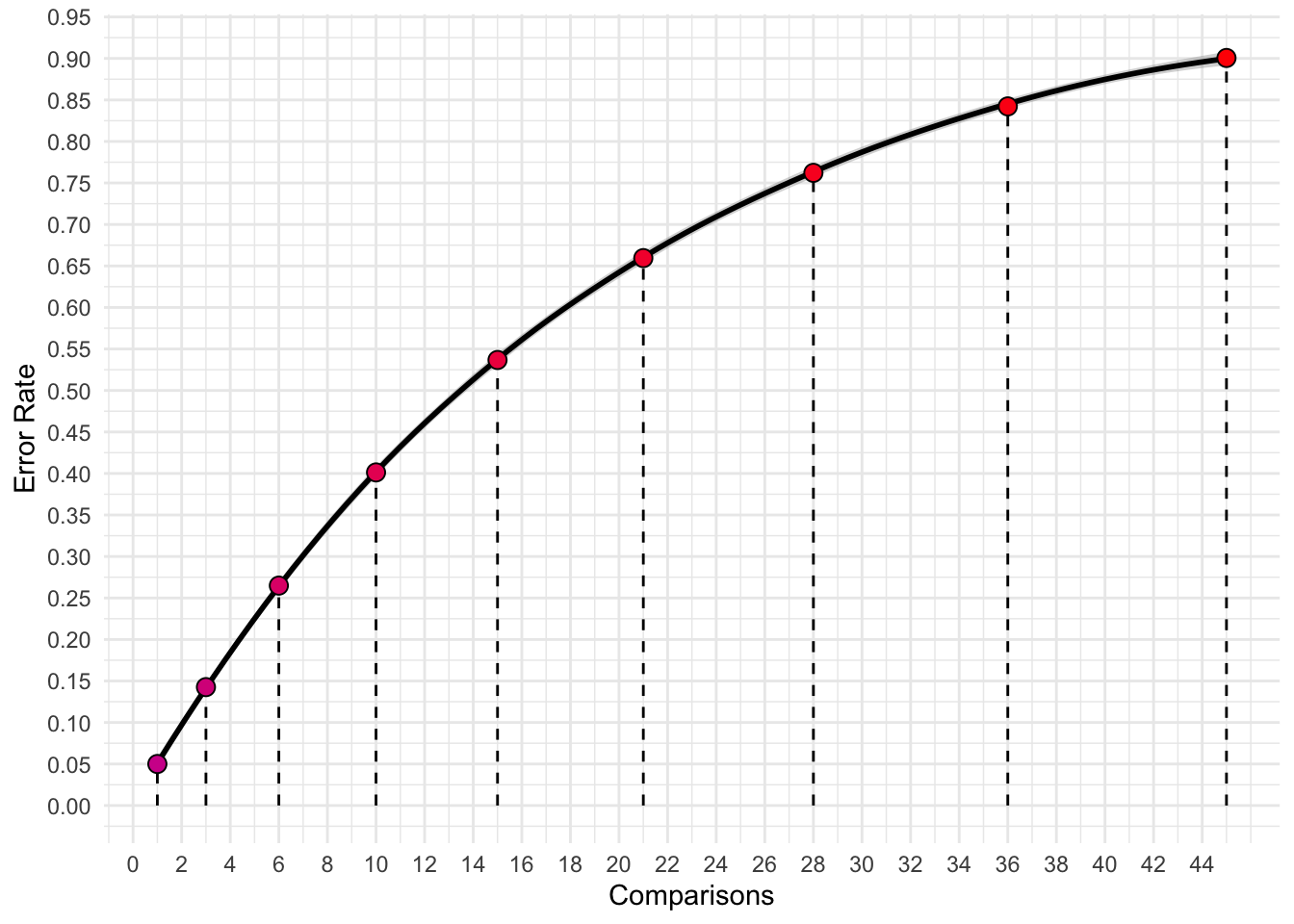
which reflect the following error rates:
| Groups | Number of Comparisons | Error Rate |
|---|---|---|
| 2 | 1 | 0.050 |
| 3 | 3 | 0.143 |
| 4 | 6 | 0.265 |
| 5 | 10 | 0.401 |
| 6 | 15 | 0.537 |
| 7 | 21 | 0.659 |
| 8 | 28 | 0.762 |
| 9 | 36 | 0.842 |
| 10 | 45 | 0.901 |
Initially, we should test only those comparisons with which we hypothesize to be different; doing more increases the likelihood that we commit a Type 1 error. However, sometimes it makes sense to also do exploratory analyses. If we conduct exploratory analyses, we should adjust our error rate to reflect the multiple comparisons.
We will cover one major method of comparing group means: Tukey’s Honestly Significant Difference (HSD).
11.8.1 Tukey’s HSD
Tukey’s HSD provides an efficient ways to compare multiple groups simultaneously to determine if their difference is statistically significant. Basically, Tukey’s HSD provides a number with which to compare differences in group means. If two groups means’ differ by more then Tukey’s HSD, then they are statistically different.
Tukey’s HSD is, essentially, all t-test comparisons using a correction for family-wise error rates.
The formula for Tukey’s HSD is:
\(T = q\times\sqrt{\frac{MSE}{n}}\)
where \(q\) is a critical q value, \(MSE\) is the mean squared error from our ANOVA, \(n\) is the sample size per group. Should the difference between the means of two groups exceed \(T\), they are considered statistically different.
From our ANOVA above, we got \(MSE=3.48\) and \(5\) individuals per group. When we look up the critical \(q\) value (for \(k=4\) and \(df_e = 16\)), we get \(q=4.047\). Thus, Tukey’s HSD would be:
\(T = q\times\sqrt{\frac{MSE}{n}}=4.047\times\sqrt{\frac{3.48}{5}}=3.376\)
Thus, we can classify any mean difference beyond 3.376 as statistically significant. Our groups are as follows:
| Mean Difference | |
|---|---|
| CBT_Rx-CBT | -1.8 |
| Placebo-CBT | 4.2 |
| Rx-CBT | 1.4 |
| Placebo-CBT_Rx | 6.0 |
| Rx-CBT_Rx | 3.2 |
| Rx-Placebo | -2.8 |
Thus, we would conclude that both the CBT group and the CBT + Rx group has statistically significant OCD Severity scores when compared to the Placebo Group. Specifically, the difference between the CBT group’s OCD severity score (\(\overline{x}_{cbt}=9.8\)) and the Placebo group (\(\overline{x}_{placebo}=14.0\)) are unlikely given a true null hypothesis, \(p<.05\). Similarly, the difference between the CBT + Rx group’s OCD severity score (\(\overline{x}_{cbt+rx}=8.0\)) and the Placebo group are unlikely given a true null hypothesis, \(p<.05\). All other groups did not differ.
While our hand calculations only give us an ‘above or below’ \(p<.05\)/\(p>.05\), a statistics program will provide a specific p-value.
11.9 Bonferonni Correction
Sometimes you may wish to do some post-hoc comparisons, but without doing Tukey’s HSD. You may also apply a Bonferonni correction to the \(\alpha\) level to attempt to control for the family wise error. To do so, simply use the following:
\(\alpha_{new}=\frac{\alpha}{n_{comparisons}}\)
So, imagine we decide post-hoc to conduct three exploratory analyses. If our original \(\alpha=.05\), then our new critical value would be \(\alpha_{new}=\frac{\alpha}{n_{comparisons}}=\frac{.05}{3}=.01667\)
11.10 Effect Size
We can calculate \(\eta^2\) (eta squared) as an effect size for our ANOVAs. This is simply the ratio of SSB and SST. That is, deviations explained by the model over all deviations. It is an indicator for fit of our model. It ranges from 0 (nothing explained by the model) to 1 (everything explained by the model).
\(\eta^2 = \frac{SSB}{SST}\)
Typically, the following cut-offs are used:
- \(\eta^2\)= .01 (small effect size)
- \(\eta^2\)= .06 (medium effect size)
- \(\eta^2\)= .14 (large effect size)
Let’s calculate it for our OCD example above. We had \(SSB=96.15\) and \(SST=SSB+SSE=96.15+55.60\). Therefore:
\(\eta^2=\frac{96.15}{151.75}=.634\)
Remember, F
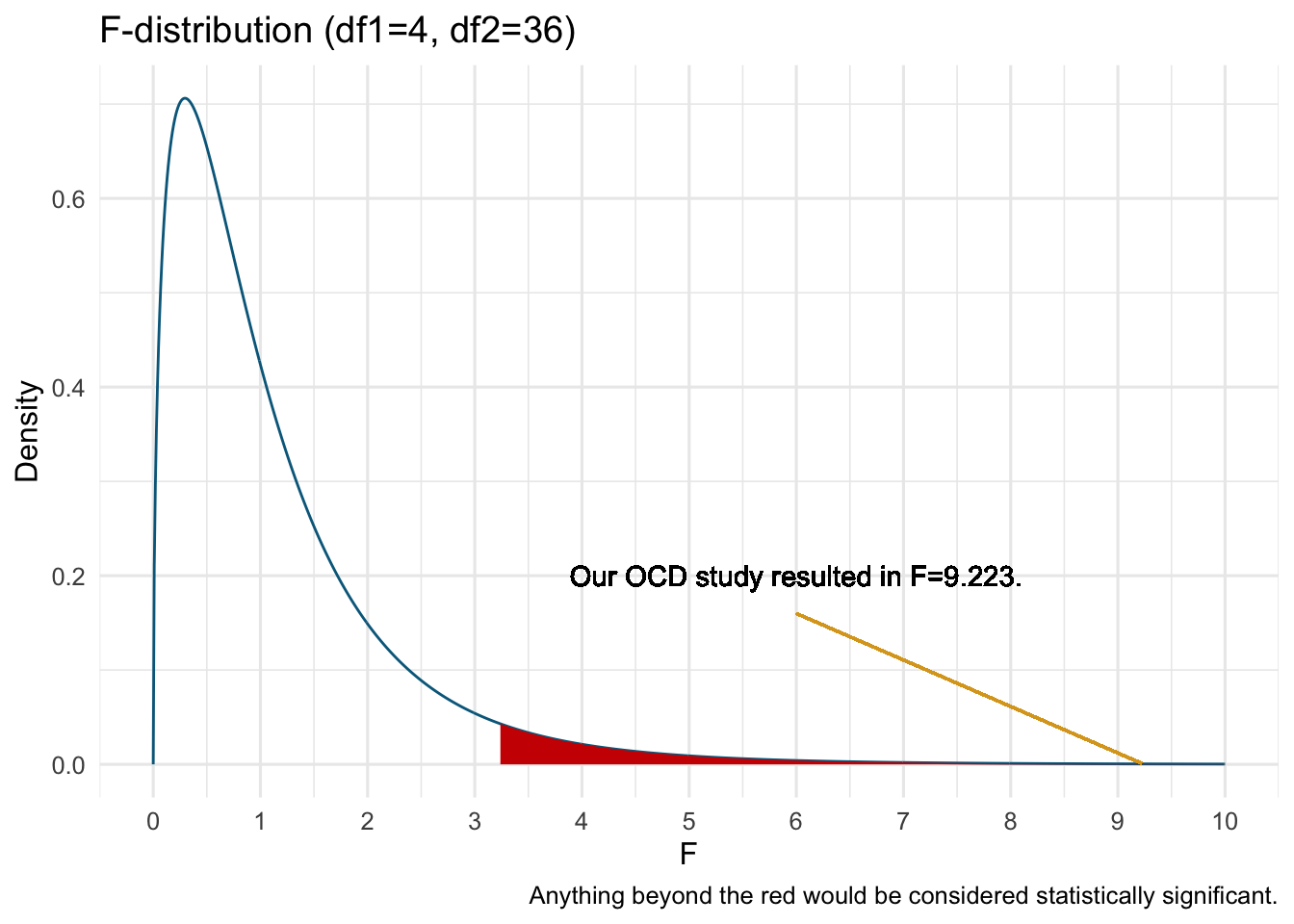
These F-distributions are expected when the two scaled chi-square distributions are completely random. The F-test, as in ANOVA, are testing the null hypothesis that the between group differences are the same as the within group differences. Considering that we randomly select and assign individuals to groups, any differences in scores within groups (i.e., the error sum of squares, SSE) are considered random and independent and would follow a chi-square distribution with \(N-p\) degrees of freedom, where N is the total sample size and p is the number of groups.
Thus, when between groups differences are larger than expected at random, we would expect a higher F-statistic. How high? Well, that depends on your alpha-level. For example, if you perform NHST with an alpha = .05, then a statistically significant result would be an F-statistic at or higher than the 95th percentile (or other criterion you set). For example, for an F-distribution with \(df_b=3\) and \(df_w = 16\) would be statistically significant if \(F\geq3.239\) (the red region, which represents 5% of the distribution):
11.11 ANOVA Model - Part 2
Surprisingly, you may learn that the ANOVA is the same as regression. In fact, we can model an ANOVA through the general linear model. In our specific example above with four treatment groups:
\(y_i=\beta_0 + x_{1i}\beta_1+x_{2i}\beta_2+x_{3i}\beta_3+e_i\)
where \(y_i\) is individual \(i\)’s score on the DV, \(e_i\) is the residual/error for individual \(i\), \(\beta_n\) are regression coefficients, and \(x_{ni}\) are individual \(i\)’s score on the \(n^{th}\) variable.
What are these variables? For an ANOVA, we would use what is known as dummy coding. In dummy coding, there will be k-1 variables, where k is the number of groups. So, in the above, we have four groups. Thus, we will have \(k-1=4-1=3\) dummy variables. In dummy coding, we choose a reference category, here we can pick placebo, and the other groups are represented by the dummy variables. Scores on dummy coded variables change depending on what group an individual is in. In our example:
| Group | Placebo | CBT | Rx | CBT + Rx |
|---|---|---|---|---|
| \(\beta_1\) | 0 | 1 | 0 | 0 |
| \(\beta_2\) | 0 | 0 | 1 | 0 |
| \(\beta_3\) | 0 | 0 | 0 | 1 |
As you can see, each group has a unique pattern on the dummy variables. So how does this fit within the GLM and regression? Well, let’s focus on the placebo group. First, recall our means:
| Treatment | Mean |
|---|---|
| CBT | 9.8 |
| CBT_Rx | 8.0 |
| Placebo | 14.0 |
| Rx | 11.2 |
For the placebo group, using our dummy coding:
\(placebo=\beta_0 + 0\beta_1+0\beta_2+0\beta_3\)
therefore
\(placebo=\beta_0\)
\(\beta_0\) is the mean of the placebo group (here, 14)!
What about the CBT group?
\(CBT=\beta_0 + 1\beta_1+0\beta_2+0\beta_3\)
therefore
\(CBT=\beta_0 + 1\beta_1\)
Well, we know that \(\beta_0\) is the mean of the placebo group (14), and we know the mean of the CBT group (9.8). Therefore:
\(CBT=\beta_0 + \beta_1\)
\(9.8=14 + \beta_1\)
\(\beta_1= 9.8-14 = -4.2\)
Interesting. \(\beta_1\) is simply the difference in means in placebo and CBT group, \(\beta_1 = \overline{x}_{CBT}-\overline{x}_{placebo}\). I hope you can intuitively figure out what \(\beta_2\) and \(\beta_3\) represent?
One important consideration here is what group we choose as the reference group (the one with no coefficient). This determines which means are being compared through each regression parameter, \(\beta\).
Practice Question
Solve for \(\beta_2\) and \(\beta_3\) in the OCD example.
We can also use the model to solve for an individual’s score. Assuming we are interested in person \(i=16\) (from the placebo group). From the above equation, we get:
\(y_{16}=\beta_0 + 0\beta_1+0\beta_2+0\beta_3+e_{16}\) (because their scores are 0 on each dummy variable.
Therefore
\(y_{16}=\beta_0+e_{16}\)
So individual 16’s score is simply, the \(\beta_0+e_16\). Interestingly, \(\beta_0\) is simply the mean of the placebo group and \(e_16\) is the deviation from the mean of the placebo group. Here:
\(y_{16}=\beta_0+e_{16}\)
and
\(12 = 14 + e_{16}\), so
\(e_{16} = 12-14=-2\)
Practice Question
Solve for individual \(1\) in the OCD example, who is part of the CBT group and who’s OCD Severity score is 12
When we cover regression, you will like see additional similarities in ANOVA and regression. All of the analysis we will cover are linked to the general linear model.
11.12 ANOVA in R
R can easily run the ANOVA and provide an ANOVA summary table. I particularly like the apa.aov.table() function from the apaTables library:
library(apaTables)
#I named my data dat_ocd
one_way_anova_example <- aov(OCD_Severity~Treatment, data=dat_ocd)
apa.1way.table(iv=Treatment, dv=OCD_Severity, data=dat_ocd)
Descriptive statistics for OCD_Severity as a function of Treatment.

 Treatment     M   SD
       CBT  9.80 2.28
    CBT_Rx  8.00 1.22
   Placebo 14.00 2.12
        Rx 11.20 1.64

Note. M and SD represent mean and standard deviation, respectively.
and:
apa.aov.table(one_way_anova_example)
ANOVA results using OCD_Severity as the dependent variable


   Predictor     SS df     MS      F    p partial_eta2 CI_90_partial_eta2
 (Intercept) 480.20  1 480.20 138.19 .000
   Treatment  96.15  3  32.05   9.22 .001          .63         [.26, .73]
       Error  55.60 16   3.48

Note: Values in square brackets indicate the bounds of the 90% confidence interval for partial eta-squared
11.12.1 Tukey’s HSD in R
Tukey’s HSD can be found in the stats library. You simply use your ANOVA model as the main argument.
library(stats)
mod_aov <- aov(OCD_Severity ~ Treatment, data=dat_ocd)

TukeyHSD(mod_aov) #I called our ANOVA model 'mod_aov'
Tukey multiple comparisons of means
95% family-wise confidence level
Fit: aov(formula = OCD_Severity ~ Treatment, data = dat_ocd)
$Treatment
diff lwr upr p adj
CBT_Rx-CBT -1.8 -5.1730926 1.5730926 0.4455114
Placebo-CBT 4.2 0.8269074 7.5730926 0.0124673
Rx-CBT 1.4 -1.9730926 4.7730926 0.6430433
Placebo-CBT_Rx 6.0 2.6269074 9.3730926 0.0005715
Rx-CBT_Rx 3.2 -0.1730926 6.5730926 0.0660661
Rx-Placebo -2.8 -6.1730926 0.5730926 0.1225197You would interpret the last column, p adj as usual. The values have been adjusted to account for family wise error rates.
11.13 Assumptions
There are three assumptions within an ANOVA we must consider:
11.13.1 1. The residuals are normally distributed
It’s a common misconception that the DV must be normally distributed. In reality, the residuals should be normally distributed. We can visualize this using a Q-Q plot or formally test this using the Shapiro-Wilks test (when sample sizes aren’t too large).
11.13.1.1 Q-Q Plot
The Q-Q plot show what a variable would like like if it were normally distributed compared with what it actually is. In essence, we order our variable and compare to what the quantiles should look like under normality. Consider the following data:
| x |
|---|
| 10.77 |
| 9.86 |
| 9.80 |
| 9.92 |
| 8.82 |
We could order these variables as: 8.82, 9.8, 9.86, 9.92, 10.77. Under a normal distribution, we would create five quantiles.
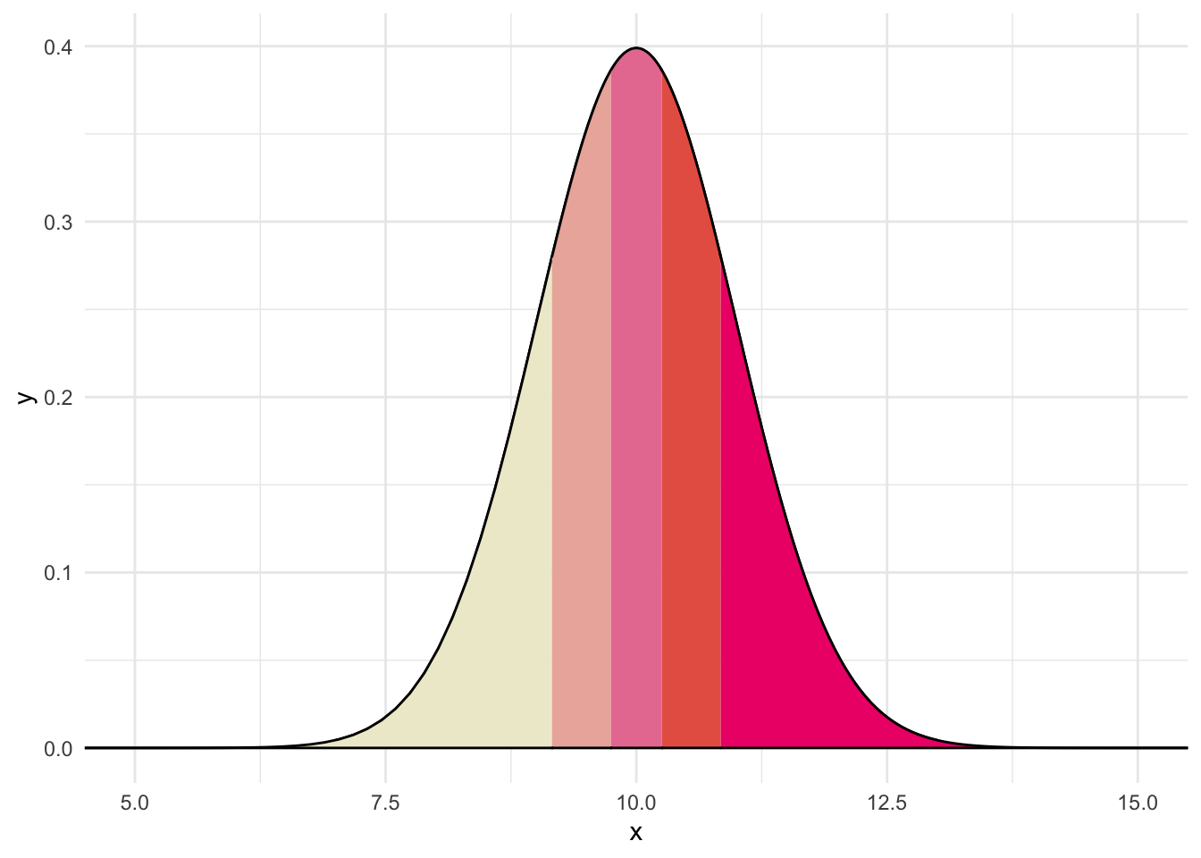
Believe it or not, each section in the above contains the same proportion. Thus, if data were normally distributed and we drew 5 numbers, like above, we would expect one to fall in each quantile. The QQ plot compares where we would expect values to fall on a normal curve versus where they actually are (e.g., z-score)
We want to conduct it on the residuals of our general model. In R:
#Setting up the model
mod_aov <- aov(OCD_Severity ~ Treatment, data=dat_ocd)

# Getting residuals of the model
residuals <- resid(mod_aov) %>%
  data.frame() %>%
  rename("residual"=".")
Let’s peek at the residual for row 16 to see if it aligns with what we calculated above for the OCD example:
residuals[16,][1] -2And we can view a Q-Q plot by using the car package:
qqPlot(residuals$residual, envelope = F)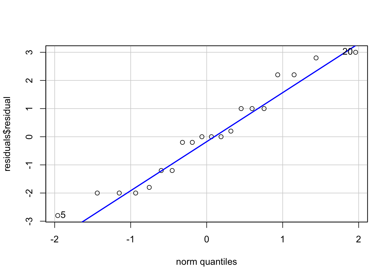
[1] 20 5There appear to be no major deviations. Normally distributed data will fall on the line. Typically, we would be concerned if the points systematically varied from the line.
11.13.1.2 Shapiro-Wilks Test
The Shapiro-Wilks test assesses how far the data deviates from normality. A statistically significant result (\(p<.05\)) is typically interpreted as the data deviating for normality. For our residuals:
#Shapiro-Wilks
shapiro.test(residuals$residual)
    Shapiro-Wilk normality test

data:  residuals$residual
W = 0.94924, p-value = 0.3557
Thus, our data do not appear to deviate from normality.
11.13.2 2. Heterogeniety of Variance
Recall that the F-distribution assumes that the data come from the same population and, thus, should have the same variance. We test this using Levene’s test. Levene’s test is part of the car package which we already loaded. The arguments look similar to the ANOVA model we built:
leveneTest(OCD_Severity~Treatment, data=dat_ocd)Warning in leveneTest.default(y = y, group = group, ...): group coerced to
factor.Levene's Test for Homogeneity of Variance (center = median)
Df F value Pr(>F)
group 3 0.9645 0.4335
16 The results suggest that the data are likely should the groups have equal variances, \(F=0.9645\), \(p=.4335\). Thus, we have not violated the assumption.
11.13.3 3. The observations are independent
Specifically, the assumption is that the residuals are independent. That is, one residual score should not be correlated with any other residual score.
11.14 Plotting the Data
There any many ways you can visualize the results of an ANOVA. One way that is not recommended is the ‘dynamite plot’.
Dynamite plot:
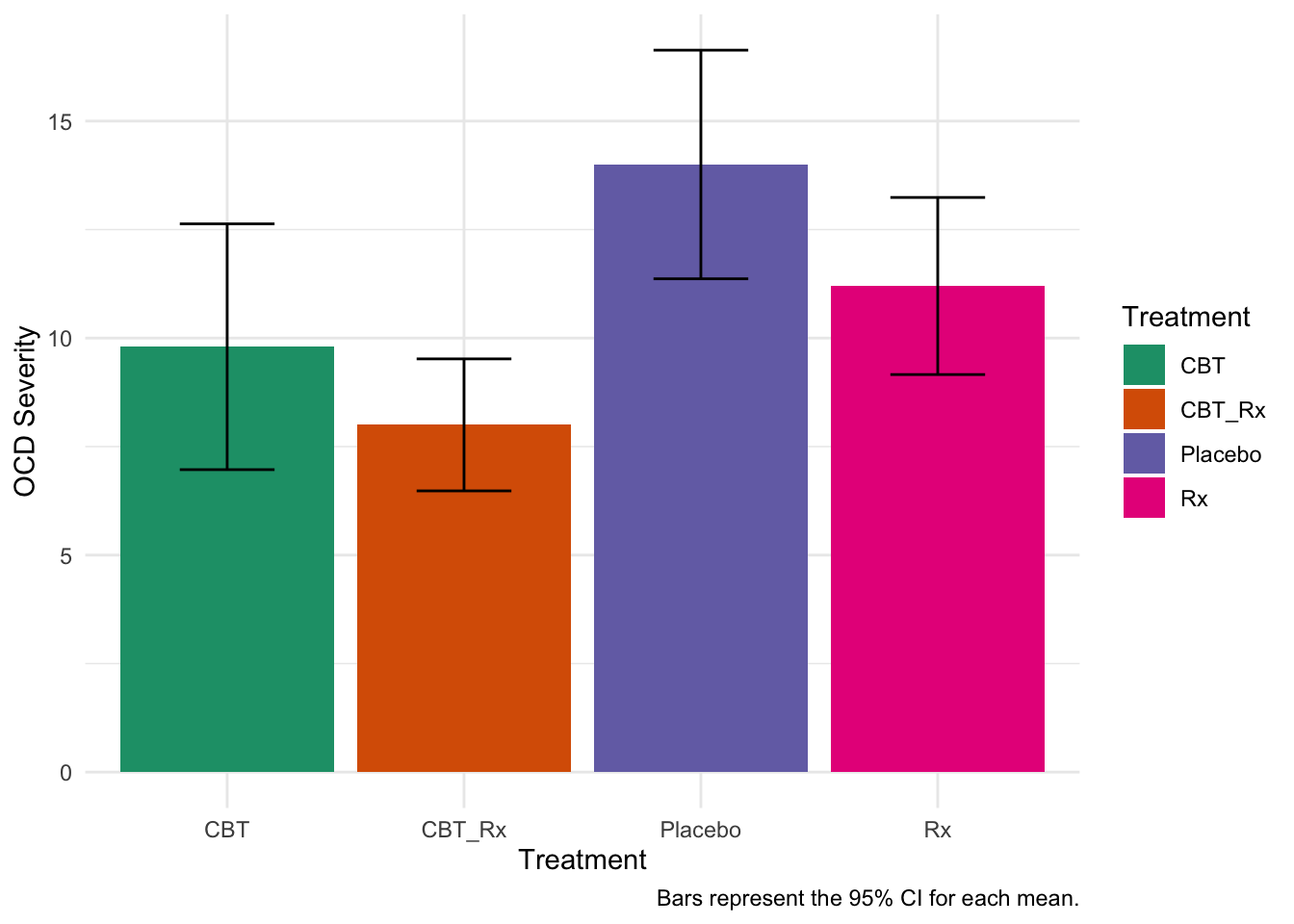
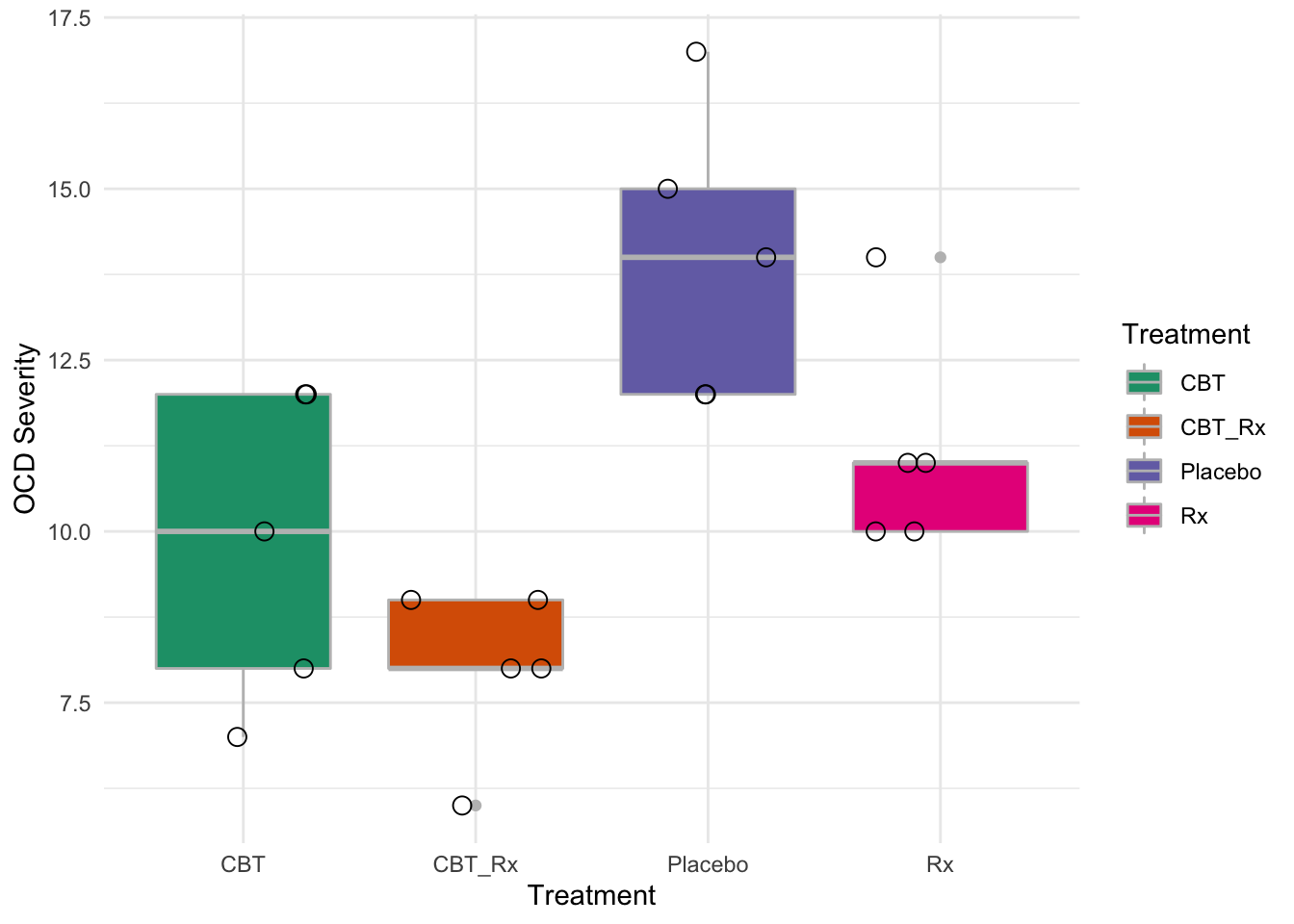
How should we visualize it? There are many ways, but one box plots may be a better method. It gives more details about the data.
11.15 Practice Question
You are a sport psychologist testing if the type of drink improves performance. You provide three drinks to sprinters and measure the time to run 100m. The following data are obtained.
| ID | Drink | Speed |
|---|---|---|
| 1 | Water | 9 |
| 2 | Water | 15 |
| 3 | Water | 16 |
| 4 | Water | 18 |
| 5 | Water | 8 |
| 6 | Milk | 19 |
| 7 | Milk | 19 |
| 8 | Milk | 18 |
| 9 | Milk | 25 |
| 10 | Milk | 20 |
| 11 | Gatorade | 13 |
| 12 | Gatorade | 12 |
| 13 | Gatorade | 19 |
| 14 | Gatorade | 8 |
| 15 | Gatorade | 15 |
Conduct an ANOVA to determine if any groups differ from any others. Specifically:
Write the null and alternative hypotheses
Conduct appropriate omnibus test
Conduct post-hoc tests.
Calculate an effect size.
Write a results section
Answers
Hypotheses
\(H_0=\mu_{water}=\mu_{milk}=\mu_{gatorade}\)
\(H_1=\) at least one different.
Omnibus
Means and F Table
Descriptive statistics for Speed as a function of Drink.

    Drink     M   SD
 Gatorade 13.40 4.04
     Milk 20.20 2.77
    Water 13.20 4.44

Note. M and SD represent mean and standard deviation, respectively.
ANOVA results using Speed as the dependent variable


   Predictor     SS df     MS     F    p partial_eta2 CI_90_partial_eta2
 (Intercept) 897.80  1 897.80 61.63 .000
       Drink 158.80  2  79.40  5.45 .021          .48         [.05, .64]
       Error 174.80 12  14.57

Note: Values in square brackets indicate the bounds of the 90% confidence interval for partial eta-squared
Results
The ANOVA (formula: Speed ~ Drink) suggests that:

  - The main effect of Drink is statistically significant and large (F(2, 12) =
5.45, p = 0.021; Eta2 = 0.48, 95% CI [0.07, 1.00])

Effect sizes were labelled following Field's (2013) recommendations.
Tukey’s HSD
  Tukey multiple comparisons of means
    95% family-wise confidence level

Fit: aov(formula = Speed ~ Drink, data = sprint)

$Drink
               diff         lwr        upr     p adj
Milk-Gatorade   6.8   0.3601802 13.2398198 0.0384112
Water-Gatorade -0.2  -6.6398198  6.2398198 0.9962235
Water-Milk     -7.0 -13.4398198 -0.5601802 0.0331468