[1] 94.5149 112.9123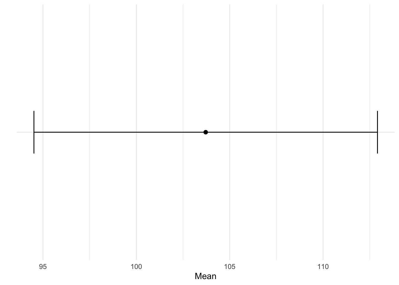
If you read the last chapter on p-values, you know that there is a limited amount of information that a p-value can tell you. Essentially, it can say whether the data is probable given a true null hypothesis. Often, we want more than that. Consider Miller and his famous research on short-term memory. Imagine if we discussed Miller’s research as that his data are unlikely if people could not hold anything in short-term memory, \(p=.03\). Not that informative when compared to a point and precision estimate: \(7\pm2\).
Confidence intervals are intervals that present the most plausible values for a given parameter based on a sample. For example, we might conduct a correlation study and determine that \(r=.3\), \(95\%CI[.2, .34]\), indicating that the best guess for the population parameter is .3, while anywhere from .2 to .34 is plausible. Typically, when working with CIs, we have:
Point estimate: a single number that indicates the derived statistic. For any given sample, it is the most plausible value of the population parameter.
Confidence interval: “an interval or range of plausible values for some quantity of population parameter of interest. A CI is a set of parameter values that are reasonably consistent with the sample data we have observed.” (Cumming & Finch, 2001).
Confidence level: the degree of certainty we wish to put around a group of CIs in the long run. Typically set to 95% to correspond with \(\alpha\) in NHST.
There are numerous potential benefits of using CIs, as Cumming and Finch (2001) explain. Let’s explore these in detail:
- They give point and interval information that is accessible and comprehensible and so, as the examples above illustrate, they support substantive understanding and interpretation. (Cumming & Finch)
Where as p-values tell us little, CIs tell us much. While p-values are generally misinterpreted or difficult to interpret, particularly for novice researchers and the general public, CIs are more easily interpretable.
For example, consider this statement. The relationship between depression and anxiety are unlikely given a true null hypothesis, \(p=.021\). That’s more more to tease apart than: the relationship between depression and anxiety is plausibly range from a small medium positive relationship, \(r=.22\), \(95\%CI[.15, .33]\).
Or consider another example. I want to know how tall you are. You say: given how tall I am, I’m probably not 0cm tall, \(p<.001\). Versus: I’m probably 162cm tall, but am plausibly between 160-165cm tall. The former is what a p-value can tell us, the latter what a CIs seeks to tell us.
- There is a direct link between CIs and familiar null hypothesis significance testing (NHST): Noting that an interval excludes a value is equivalent to rejecting a hypothesis that asserts that value as true—at a significance level related to C. A CI may be regarded as the set of hypothetical population values consistent, in this sense, with the data. (Cumming & Finch)
What is meant here, is that if I CI excludes a null hypothesis value at whatever confidence level (e.g., 95%), it would also reject that value through NHST and the same \(\alpha\) level. For example, if you concluded that the mean difference between two groups is \(\overline{x}_{diff}=.3\), \(95\%CI[.1, .38]\), then a standard NHST would results in \(p<.05\) for the same test. If the CIs excludes 0, you would get a statistically significant result.
The CI tells you just as much, and much more, than a p-value.
- CIs are useful in the cumulation of evidence over experiments: They support meta-analysis and meta-analytic thinking focused on estimation. This feature of CIs has been little explored or exploited in the social sciences but is in our view crucial and deserving of much thought and development. (Cumming & Finch)
CIs propose that their values will inform of population parameters over the long run. Meta-analysis can facilitate this by pooling multiple studies into one strong evidence base. Because a 95%CI indicates that 95% of CIs over the long run will contain the true population parameter, meta-analysis can inform just where that parameter may be. Forrest plots are helpful in this regard.
- CIs give information about precision. They can be estimated before conducting an experiment and the width used to guide the choice of design and sample size. After the experiment, they give information about precision that may be more useful and accessible than a statistical power value. (Cumming & Finch)
Given we know that CIs are made up of point estimates and intervals, we can visualize them to help us understand what they are. Imagine a population (e.g., all Grenfell students). We want to sample from the population and infer from the sample statistics about the population parameter. Our hypothetical construct of interest is intelligence quotient. Imagine that we know the population parameters: \(\overline{X}_{IQ}=105\) and \(\sigma_{IQ}=15\).
If we sample from the population we can calculate a CI. Let’s assume we calculate the 95% CI. We may get a mean of 103.71, with a 95% CI of [94.51, 112.91]. Let’s visualize it:
[1] 94.5149 112.9123
Imagine that instead of taking one sample, we re-ran the study over, and over, and over…. 100 times!! If we plot the CIs for each of these studies, we get this. For conveience, I’ll put a solid verticle line to represent the known population mean:
 No Yes
5 95 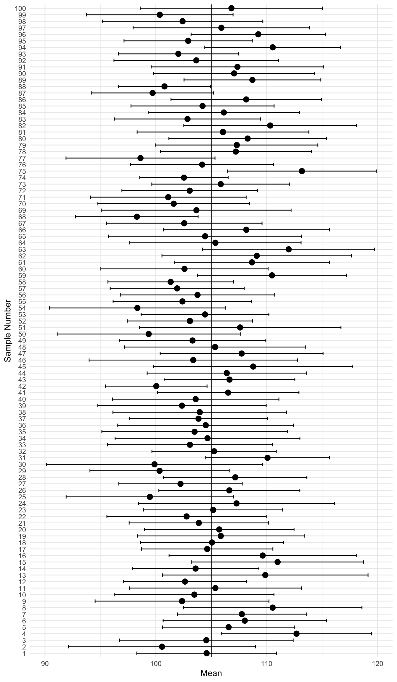
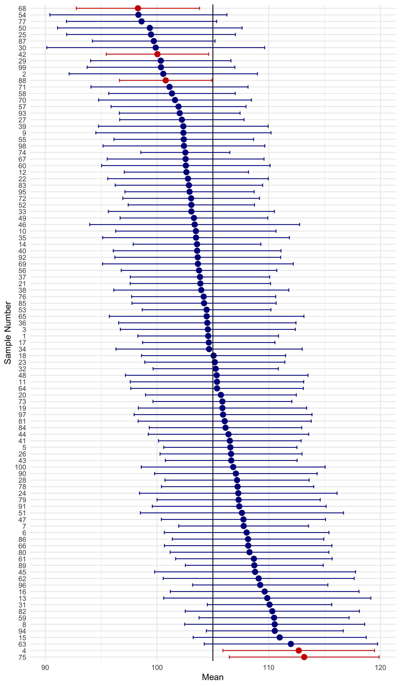
You may notice that some of the CIs contain the true population parameter and some do not. It may be easier to see when I sort them by their mean.
Stop and think before moving on. How many of the CIs contain the true population parameter?
…keep thinking…
…keep thinking…
There are 95/100, 95%, confidence intervals that contain the true parameter. This is the meaning of a CI.
A CI tells you nothing about the probability of any single CI containing the parameter.
It tells you the most plausible values of the parameter for a given sample.
Also, the % of CIs containing the parameter will equal the confidence level.
If we adjusted our CIs to be 99% versus 95%, we can adjust the SEs and replot them:
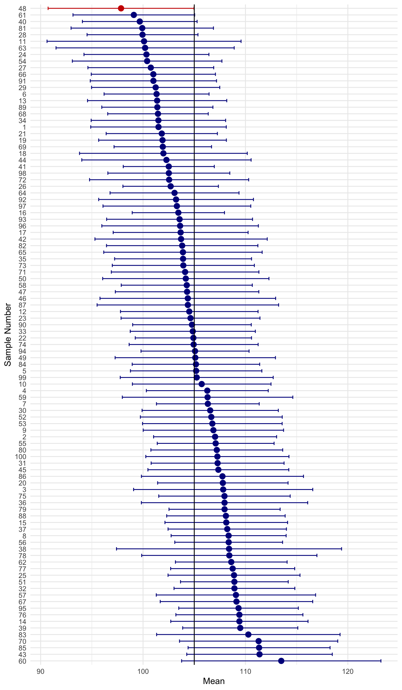
By adjusting the SEs on new data 99/100 (i.e., 99%) contain the parameter.
Let’s work out how to calculate CIs for some common metrics. While we will not learn how to calculate them for more advanced statistics, the rationale it typically the same: the statistics \(\pm\) margin of error.
\(\overline{x} \pm =t_{(n-1, \frac{\alpha}{2})}(\frac{s}{\sqrt{n}})\)
where
\(t_{(n-1, \frac{\alpha}{2})}\) is the critical \(t\) value for \(n-1\) df and \(\alpha\) is your 1- your CI interval (e.g., .05).
Imagine the following data: 8, 5, 9, 5, 4
We need to calculate a few things. We need the mean, \(n\), the SD, the SE, and critical \(t\).
\(\overline{x}=6.2\)
\(s=2.1679\)
\(se = \frac{s}{\sqrt{n}}=\frac{2.1679}{\sqrt{5}}=0.9694\)
Next we need critical \(t\). Look up in the t-distribution table for \(\alpha/2\) and \(n-1\) degrees of freedom.
\(t_{crit}=\) 2.7764451
Our CI is:
\(\overline{x}\pm t_{(n-1, \frac{\alpha}{2})}(\frac{s}{\sqrt{n}})\)
\(=6.2\pm 2.776(0.9694)\)
\(=[3.51, 8.89]\)
Calculate the mean and 95% CI for the following list of numbers:
10, 3, 4, 3, 7
  Mean      SD N       SE  LowerCI  UpperCI
1  5.4 3.04959 5 1.363818 1.613434 9.186566