| ID | Drug | Sex | Pre | Post | Follow |
|---|---|---|---|---|---|
| 1 | New | Male | 14 | 8 | 18 |
| 2 | New | Male | 12 | 0 | 7 |
| 3 | New | Male | 16 | 6 | 12 |
| 4 | New | Male | 16 | 8 | 14 |
| 5 | New | Male | 3 | 0 | 5 |
| 6 | New | Female | 17 | 17 | 2 |
| 7 | New | Female | 13 | 14 | 10 |
| 8 | New | Female | 14 | 13 | 8 |
| 9 | New | Female | 8 | 7 | 3 |
| 10 | New | Female | 16 | 19 | 14 |
| 11 | TAU | Male | 12 | 9 | 12 |
| 12 | TAU | Male | 16 | 13 | 10 |
| 13 | TAU | Male | 16 | 11 | 7 |
| 14 | TAU | Male | 17 | 12 | 10 |
| 15 | TAU | Male | 21 | 16 | 17 |
| 16 | TAU | Female | 17 | 12 | 7 |
| 17 | TAU | Female | 11 | 8 | 1 |
| 18 | TAU | Female | 12 | 9 | 3 |
| 19 | TAU | Female | 13 | 10 | 6 |
| 20 | TAU | Female | 12 | 2 | 3 |
12 Mixed ANOVA
12.1 Background
So far we have explored independent/between-measures designs, wherein individuals in each level (i.e., group, condition, or treatment) of a factor are different. We have also explored repeated-measures/within designs, wherein individuals comprise each level of a factor. Mixed designs combine both: they have at least one between and one within-level factor. Thus, these designs are factorial by definitions (have at least two IVs).
We will not focus on the complexities of calculating test statistics by hand in this chapter. However, you should know when to use this design, and how to interpret results.
12.2 Our Data
We have developed a new anti-depressant drug that somehow binds to testosterone in the body to be effective. Theoretically, this drug should be more effective for men than women. We want to test this drug compared to treatment as usual (TAU), which is a standard SSRI. We will measure depression scores (scale of 0-25; lower scores equal lower despressive symptoms) prior to our drug trial, then after 6 months of using either drug. We also measure at 12-month follow-up. We will also compare men and women. We recruit 20 individuals (10 men and 10 women). Our data are as follows:
Click to view our data
Click to see data for copying into your own R
set.seed(362736)
df_drug <- data.frame(ID=1:20,
                      Drug = rep(c("New", "TAU"), each=10),
                      Sex = rep(c("Male", "Female", "Male", "Female"), each=5),
                      Pre = round(rnorm(20, 15, 4))) %>%
   mutate(error=rnorm(20, 0, 4),
         error2=rnorm(20, 0, 4),
           mult = rep(c(-6, 1, -3, -3), each=5)) %>%
  mutate(Post = round(Pre+mult+error)) %>%
  mutate(Follow=ifelse(Sex=="Male",
                       round(Post-2+error2),
                       round(Post+2+error2))) %>%
  dplyr::select(-error, -error2, -mult)
Thus, we have a 2 (sex) x 2 (pre/post) x 2 (New Drug vs TAU) design, with two between factors (sex and drug) and one within factor (pre/post).
12.3 Our Hypotheses
Specifically, we hypothesize that there will be main effect of time (a reduction in symptoms). However, the new drug will be more effective for men and the old drug will be equally effective for men and women (an interaction).
\(H_0:\) all \(\mu\) equal
\(H_{A1}: \mu_{Pre}<\mu_{Post}<\mu_{Follow}\)
\(H_{A2}: \Delta\mu_{(new,men)}>\Delta\mu_{(new,women)}\)
12.4 Our Model
Building on the general linear model:
\(y_i=\beta_0+\beta_{drug}(x_{1i})+\beta_{time}(x_{2i})+\beta_{sex}(x_{3i})+\beta_{dxt}(x_{1i})(x_{2i})+\beta_{dxs}(x_{1i})(x_{3i})+\beta_{sxt}(x_{2i})(x_{3i})+e_i+\beta_{dxtxs}(x_{1i})(x_{2i})(x_{3i})\)
- This may look complex, but we have a \(\beta\) for each main effect and interaction (3, 2-way interactions and 1, 3-way interaction).
12.5 Our Analyses
Let’s explore the data:
| Sex | Time | Drug | Mean | SD |
|---|---|---|---|---|
| Female | Pre | TAU | 13.0 | 2.35 |
| Female | Post | TAU | 8.2 | 3.77 |
| Female | Follow | TAU | 4.0 | 2.45 |
| Female | Pre | New | 13.6 | 3.51 |
| Female | Post | New | 14.0 | 4.58 |
| Female | Follow | New | 7.4 | 4.98 |
| Sex | Time | Drug | Mean | SD |
|---|---|---|---|---|
| Male | Pre | TAU | 16.4 | 3.21 |
| Male | Post | TAU | 12.2 | 2.59 |
| Male | Follow | TAU | 11.2 | 3.70 |
| Male | Pre | New | 12.2 | 5.40 |
| Male | Post | New | 4.4 | 4.10 |
| Male | Follow | New | 11.2 | 5.26 |
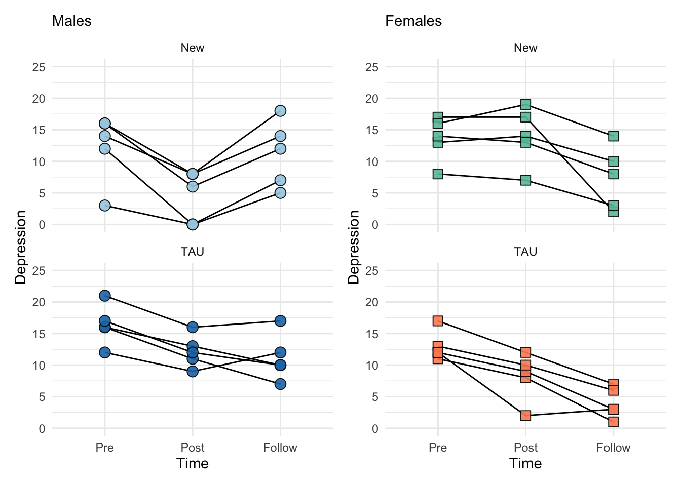
Based on your visual exploration, what might you be expecting to happen (knowing that, obviously, we will conduct formal analyses)? What trends do you notice based on the different groups?
Now that we have explored the data, we must set up our contrasts. By default, R uses dummy coding. However, dummy coding doesn’t work well with type III sums of squares, which is what we want to model an interaction. We must use an orthogonal contrast (we will use effects coding). While we won’t be setting contrasts specifically in this class, you should be familiar with them for potential honours projects in the future. For a detailed exploration of contrasts, go here.
To analyze, we can use ezANOVA() from the ez package.
ezANOVA(data=data_long,
        dv=Depression,
        wid=.(ID),
        between = .c(Sex, Drug),
        within=Time,
        type = 3,
        detailed = T)
Which gives the following output:
| ANOVA.Effect | ANOVA.DFn | ANOVA.DFd | ANOVA.SSn | ANOVA.SSd | ANOVA.F | ANOVA.p | ANOVA.ges | |
|---|---|---|---|---|---|---|---|---|
| 1 | (Intercept) | 1 | 16 | 6805.350 | 586.8 | 185.558 | 0.000 | 0.900 |
| 2 | Sex | 1 | 16 | 22.817 | 586.8 | 0.622 | 0.442 | 0.029 |
| 3 | Drug | 1 | 16 | 2.017 | 586.8 | 0.055 | 0.818 | 0.003 |
| 5 | Time | 2 | 32 | 313.300 | 166.0 | 30.198 | 0.000 | 0.294 |
| 4 | Sex:Drug | 1 | 16 | 198.017 | 586.8 | 5.399 | 0.034 | 0.208 |
| 6 | Sex:Time | 2 | 32 | 172.633 | 166.0 | 16.639 | 0.000 | 0.187 |
| 7 | Drug:Time | 2 | 32 | 33.633 | 166.0 | 3.242 | 0.052 | 0.043 |
| 8 | Sex:Drug:Time | 2 | 32 | 76.433 | 166.0 | 7.367 | 0.002 | 0.092 |
12.5.1 Assumptions
Sphericity
ezANOVA automatically provides Mauchley’s tests for each repeated value:
Warning: Converting "ID" to factor for ANOVA.| Mauchly.s.Test.for.Sphericity.Effect | Mauchly.s.Test.for.Sphericity.W | Mauchly.s.Test.for.Sphericity.p | |
|---|---|---|---|
| 5 | Time | 0.827 | 0.241 |
| 6 | Sex:Time | 0.827 | 0.241 |
| 7 | Drug:Time | 0.827 | 0.241 |
| 8 | Sex:Drug:Time | 0.827 | 0.241 |
Based on the results of Mauchley’s test, we have not violated this assumption.
Normality
Attaching package: 'rstatix'The following object is masked from 'package:MASS':
selectThe following object is masked from 'package:stats':
filter# A tibble: 12 × 6
Drug Sex Time variable statistic p
<fct> <fct> <fct> <chr> <dbl> <dbl>
1 New Female Follow Depression 0.942 0.678
2 TAU Female Follow Depression 0.925 0.563
3 New Male Follow Depression 0.963 0.829
4 TAU Male Follow Depression 0.927 0.579
5 New Female Post Depression 0.952 0.749
6 TAU Female Post Depression 0.895 0.382
7 New Male Post Depression 0.782 0.0571
8 TAU Male Post Depression 0.984 0.955
9 New Female Pre Depression 0.914 0.492
10 TAU Female Pre Depression 0.813 0.103
11 New Male Pre Depression 0.790 0.0670
12 TAU Male Pre Depression 0.940 0.666 We have not violated this assumption.
Homogeneity of Variance
For Sex:
data_long %>%
  group_by(Time) %>%
  levene_test(Depression~Sex)
# A tibble: 3 × 5
Time df1 df2 statistic p
<fct> <int> <int> <dbl> <dbl>
1 Follow 1 18 8.33e- 3 0.928
2 Post 1 18 7.64e-31 1.00
3 Pre 1 18 3.28e- 1 0.574For Drug:
data_long %>%
  group_by(Time) %>%
  levene_test(Depression~Drug)
# A tibble: 3 × 5
Time df1 df2 statistic p
<fct> <int> <int> <dbl> <dbl>
1 Follow 1 18 0.305 0.587
2 Post 1 18 2.55 0.127
3 Pre 1 18 0.0304 0.864Thus, all of our major assumptions are fine, so let’s move along.
Note: we could set this up as a multi-level model. Although I recommend this, it is beyond the scope of this class.
12.6 Our Results
Wow! I’m sure the main output from ezANOVA feels quite overwhelming on first look. However, it is quite straightforward and, from here on in this anlaysis, there is nothing that we have not yet done/encountered.
12.6.1 Main Effects
12.6.1.1 Hypothesis 1 - Symptoms will decrease over time
We will explore all main effects for the purposes of learning, but note that we are interested particularly in the main effect of time (see hypotheses).
Before looking at the main effects, it’s important to understand that main effects, significant or not, have little interpretation value when interactions are present. Thus, while we can report these, please do not put to much weight into them.
Sex
Based on our output above, we know there was no effect of sex on response to the drug, \(F(1, 16)= 0.622\), \(p= 0.442\), \(\eta^2_g=0.029\). If we ignored all other variables in the model and looked only at the differences between men and women, there would not be an effect.
Drug
Furthermore, there seem to be no main effect of drug, \(F(1, 16)=0.055\), \(p=0.818\), \(\eta^2_g= 0.003\). If we ignored sex and time, all other variables in the model and looked only at the differences between TAU and the new drug, there would not be an effect.
Time
There was a statistically significant main effect of time, \(F(2, 32)=30.20\), \(p<.001\), \(\eta^2_g= 0.294\). If we ignored sex and drug time, depression scores would vary across time.
Let’s look at these difference in more detail.
# A tibble: 3 × 6
  Time    Mean    SD    SE SE_LL SE_UL
  <fct>  <dbl> <dbl> <dbl> <dbl> <dbl>
1 Follow  8.45  4.97 1.11   7.34  9.56
2 Post    9.7   5.18 1.16   8.54 10.9
3 Pre 13.8 3.83 0.857 12.9 14.7 library(ggdist)
ggplot(data_long, aes(x=fct_relevel(Time, "Pre", "Post"), y=Depression))+
stat_halfeye(side = "left", justification=1.1,
aes(fill=Time))+
stat_dots(dotsize=.1, binwidth=3, justification=-0.01,
aes(fill=Time))+
scale_fill_brewer(palette = "Dark2")+
scale_y_continuous(breaks = seq(0, 30, 2))+
theme_minimal()+
labs(x="Time")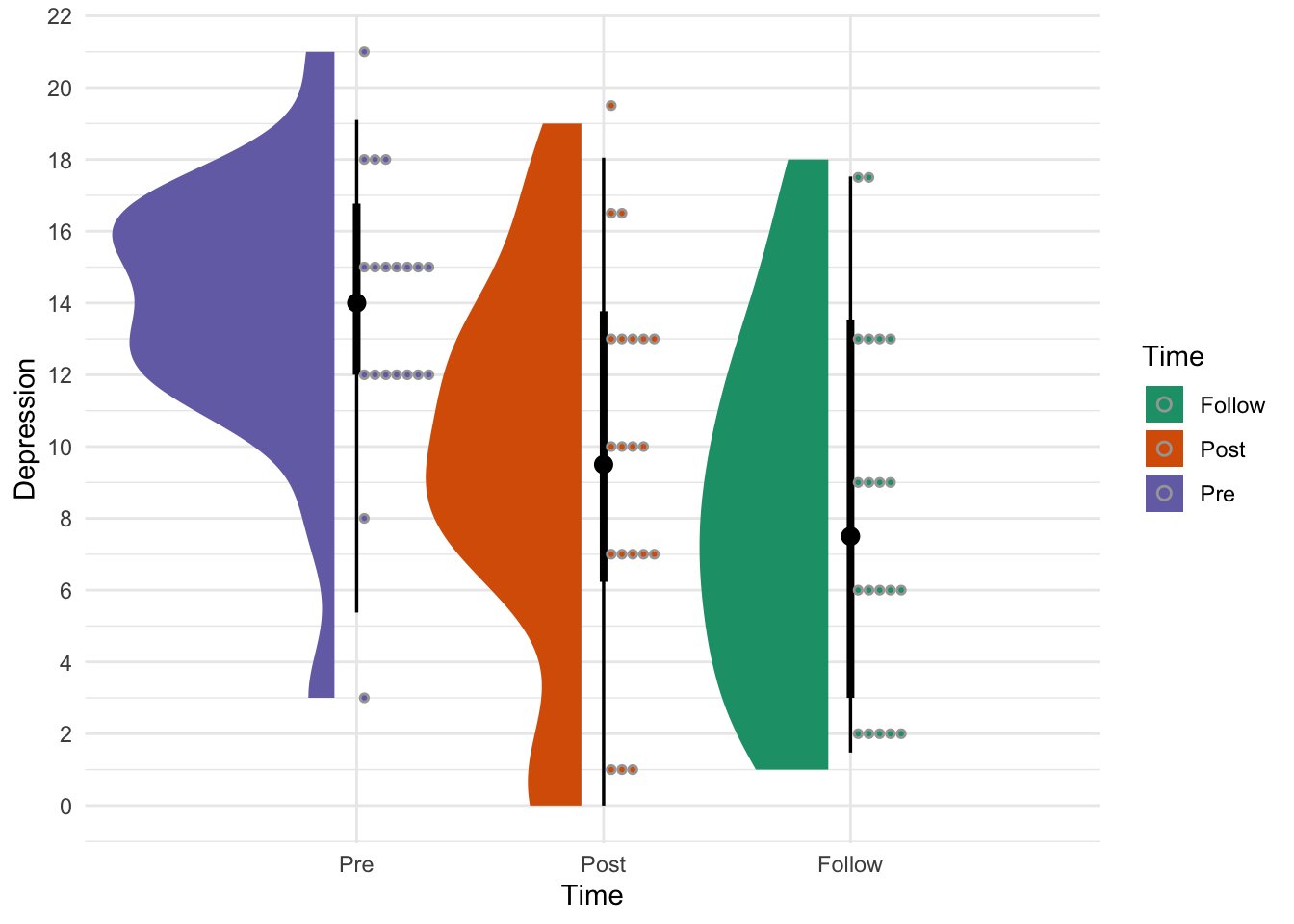
You may notice that there seems to be a downward trend, such that depression scores go down from pre, to post, to followup. We can complete post-hoc analyses by running a Tukey’s test for the within-subject variable:
TukeyHSD(aov(Depression~Time, data=data_long)) Tukey multiple comparisons of means
95% family-wise confidence level
Fit: aov(formula = Depression ~ Time, data = data_long)
$Time
diff lwr upr p adj
Post-Follow 1.25 -2.3254803 4.82548 0.6791010
Pre-Follow 5.35 1.7745197 8.92548 0.0018993
Pre-Post 4.10 0.5245197 7.67548 0.0209034Please see the repeated measures ANOVA section of this companion for additional details on reported this output. However, there is a statistically significant reduction in depressive symptoms from the Pre to Post periods, and the Pre to Follow-up periods. However, Post and Follow-Up did not differ.
NOTE: this effect is qualified by significant interactions, which requires additional in-depth exploration.
12.6.2 Two-Way Interactions
12.6.3 Hypothesis 2 - New drug more effective for men
Sex x Drug
The output suggests a significant two-way interaction between sex and drug, \(F(1,16)=5.399\), \(p=.034\), \(\eta^2_g=.208\).
We can investigate this like we did a factorial ANOVA. Our output is as follows:
# A tibble: 2 × 10
Drug .y. group1 group2 n1 n2 p p.signif p.adj p.adj.si…¹
* <fct> <chr> <chr> <chr> <int> <int> <dbl> <chr> <dbl> <chr>
1 New Depression Female Male 15 15 0.241 ns 0.241 ns
2 TAU Depression Female Male 15 15 0.00396 ** 0.00396 **
# … with abbreviated variable name ¹p.adj.signifThe above uses a Bonferonni adjust p-values. The results suggest that males and females did not differ in response to the new drug, \(p=.241\). However, females did respond more favorably to the treatment as usual, \(p=.004\). Please see the factorial ANOVA chapter for more details on conducting and writing up a two-way interaction.
Drug x Time
There was no statistically significant drug x time interaction, \(F(2, 32)=3.24\), \(p=.052\), \(\eta^2_g=.043\).
Sex x Time
The output suggests a significant two-way interaction between sex and time, \(F(2,32)=7.37\), \(p=.002\), \(\eta^2_g =.092\). We will explore this in detail; note that this is exploratory analyses versus planned analyses.
We can investigate this like we did a factorial ANOVA. Our output is as follows:
# A tibble: 3 × 10
  Time   .y.        group1 group2    n1    n2     p p.signif p.adj p.adj.signif
* <fct>  <chr>      <chr>  <chr>  <int> <int> <dbl> <chr>    <dbl> <chr>
1 Follow Depression Female Male      10    10 0.009 **       0.009 **
2 Post   Depression Female Male      10    10 0.237 ns       0.237 ns
3 Pre    Depression Female Male      10    10 0.574 ns       0.574 ns
The above uses a Bonferonni adjust p-values. The results suggest that males and females did not differ in response during the ‘Pre’ stage, \(p=.574\) nor the ‘Post’ stage, \(p=.237\). However, females did respond move favorably during the ‘Follow-up’ stage of treatment, \(p=.009\). Please see the factorial ANOVA chapter for more details on conducting and writing up a two-way interaction.
12.6.4 Three-Way Interaction
The three-way interaction will help clarify the complete picture of the results. Remember, main effects are largely unterpretable the context of interactions. Well, higher-order interactions may better explain a lower-order interaction. Remember, we had main effects of Time, but males and females only differed in the Follow-up (two-way interaction above).
The following figure will make a reappearance.

In essence, we will be asking if any differences in depression scores for Sex x Time depend on the drug. Or, similarly, if any differences in Drug x Sex depend on time.
Sex x Time for New Drug
# two-way repeated for sex/time, new drug

ezANOVA(data=data_long %>%
          filter(Drug=="New"),
        dv=Depression,
        between = Sex,
        within = Time,
        wid = ID)
Warning: Converting "ID" to factor for ANOVA.$ANOVA
Effect DFn DFd F p p<.05 ges
2 Sex 1 8 0.8289095 0.3891956032 0.07573633
3 Time 2 16 6.4474002 0.0088389822 * 0.14424846
4 Sex:Time 2 16 16.5562273 0.0001268898 * 0.30209161
$`Mauchly's Test for Sphericity`
Effect W p p<.05
3 Time 0.6840666 0.2647551
4 Sex:Time 0.6840666 0.2647551
$`Sphericity Corrections`
Effect GGe p[GG] p[GG]<.05 HFe p[HF] p[HF]<.05
3 Time 0.7599169 0.0169604905 * 0.901096 0.0115468971 *
4 Sex:Time 0.7599169 0.0006238282 * 0.901096 0.0002440033 *So, for the new drug, we have a sex by drug interaction. Let’s tease this apart with post-hoc pairwise comparisons.
## pairwise comparison

pwc1 <- data_long %>%
  filter(Drug=="New") %>%
  group_by(Time) %>%
  pairwise_t_test(Depression~Sex, paired=FALSE,
                  p.adjust.method = 'bonferroni')

pwc1
# A tibble: 3 × 10
Time .y. group1 group2 n1 n2 p p.signif p.adj p.adj.s…¹
* <fct> <chr> <chr> <chr> <int> <int> <dbl> <chr> <dbl> <chr>
1 Follow Depression Female Male 5 5 0.275 ns 0.275 ns
2 Post Depression Female Male 5 5 0.00818 ** 0.00818 **
3 Pre Depression Female Male 5 5 0.64 ns 0.64 ns
# … with abbreviated variable name ¹p.adj.signifThus, it seems that males and females only differed at the post time for the new drug, with females having higher depression scores. Note that you will need to write up each in proper t-test style.
Let’s determine if the changes over time differed for males and females.
pwc2 <- data_long %>%
  filter(Drug=="New") %>%
  group_by(Sex) %>%
  pairwise_t_test(Depression~Time, paired=TRUE,
                  p.adjust.method = 'bonferroni')

pwc2
# A tibble: 6 × 11
Sex .y. group1 group2 n1 n2 statis…¹ df p p.adj p.adj…²
* <fct> <chr> <chr> <chr> <int> <int> <dbl> <dbl> <dbl> <dbl> <chr>
1 Female Depression Follow Post 5 5 -3.13 4 0.035 0.106 ns
2 Female Depression Follow Pre 5 5 -2.68 4 0.055 0.165 ns
3 Female Depression Post Pre 5 5 0.535 4 0.621 1 ns
4 Male Depression Follow Post 5 5 7.90 4 0.001 0.004 **
5 Male Depression Follow Pre 5 5 -0.577 4 0.595 1 ns
6 Male Depression Post Pre 5 5 -4.99 4 0.008 0.023 *
# … with abbreviated variable names ¹statistic, ²p.adj.signifThus, females had no statistically significant changes in depressive symptoms across any time points. However, males had a significant reduction in symptoms from pre to post, but an increase from post to follow.
Sex x Time for TAU
# two-way repeated for sex/time, new drug

ezANOVA(data=data_long %>%
          filter(Drug=="TAU"),
        dv=Depression,
        between = Sex,
        within = Time,
        wid = ID)
Warning: Converting "ID" to factor for ANOVA.$ANOVA
Effect DFn DFd F p p<.05 ges
2 Sex 1 8 8.365777 2.012599e-02 * 0.44052244
3 Time 2 16 37.043062 9.901401e-07 * 0.53356306
4 Sex:Time 2 16 2.995215 7.853984e-02 0.08466324
$`Mauchly's Test for Sphericity`
Effect W p p<.05
3 Time 0.892768 0.6723342
4 Sex:Time 0.892768 0.6723342
$`Sphericity Corrections`
Effect GGe p[GG] p[GG]<.05 HFe p[HF] p[HF]<.05
3 Time 0.9031531 2.956562e-06 * 1.150909 9.901401e-07 *
4 Sex:Time 0.9031531 8.557843e-02 1.150909 7.853984e-02 So, for TAU, we have a main effect of sex and time, but no interaction. We can conduct post hoc tests to determine the nature of these main effects.
# Main effect sex

data_long %>%
  filter(Drug=="TAU") %>%
  pairwise_t_test(Depression~Sex, paired=F)
# A tibble: 1 × 9
.y. group1 group2 n1 n2 p p.signif p.adj p.adj.signif
* <chr> <chr> <chr> <int> <int> <dbl> <chr> <dbl> <chr>
1 Depression Female Male 15 15 0.00396 ** 0.00396 ** Thus, the means of males (\(\overline{x}=13.30\)) was higher than females (\(\overline{x}=8.40\)).
For the main effect of time, we can conduct post-hoc analyses.
pwc_time <- data_long %>%
  filter(Drug=="TAU") %>%
  pairwise_t_test(Depression~Time, paired=TRUE,
                  p.adjust.method = 'bonferroni')

pwc_time
# A tibble: 3 × 10
.y. group1 group2 n1 n2 statistic df p p.adj p.adj…¹
* <chr> <chr> <chr> <int> <int> <dbl> <dbl> <dbl> <dbl> <chr>
1 Depression Follow Post 10 10 -2.49 9 0.035 0.104 ns
2 Depression Follow Pre 10 10 -7.14 9 0.000054 0.000162 ***
3 Depression Post Pre 10 10 -6.55 9 0.000105 0.000315 ***
# … with abbreviated variable name ¹p.adj.signifWe can see that depressive score were lower for teh Pre time when compared to the Post and Follow-up time. However, the Post and Follow-up up times were not statistically significant when accounting for the Bonferroni correction.
We now have enough information to answer our initial hypotheses.
12.7 Our Write-up
All tests are tests are reported as significant at \(p<.05\); Bonferroni corrections were used for multiple comparisons.
We first hypothesized a main effect of Time on depressive symptoms, such that depressive symptoms would decrease over time. Indeed, the main effect of time was statistically significant, \(F(2, 32)=30.20, p<.001, \eta^2_g=.294\). Specifically, depressive symptoms were lower at the Pre time (\(\overline{x}=13.8, SD=3.83\)) when compared to the Post (\(\overline{x}=9.7, SD=5.18, p=.021\)) and Follow-up (\(\overline{x}=8.45, SD=4.97, p=.002\)) times.
Second, we hypothesized that the new drug would be more effective for men in long term, while the old drug would not vary over time between men and women. For the new drug, while there was a significant main effect for time, \(F(2, 16)=6.45, p=.009, \eta^2_g=.144\), females had no statistically significant changes in depressive symptoms across time point, while males experiences a significant decrease in symptoms from Pre to Post and Increase from Post to Follow-up. The Pre and Follow-up scores did not differ for males. males experience lower depressive symptoms when compared to women at the Post time, while other differences existed.
For TAU, there was a main effect of sex, \(F(1, 8)=8.37, p=.020, \eta^2_g=.440\), with females (\(\overline{x}=8.40\)) having significantly lower depressive symptoms than males (\(\overline{x}=13.30\)). There was a main effect of time on depressive symptoms, \(F(2, 16)=37.04, p<.001, \eta^2_g=.534\). Here, individuals experiences a reduction in symptoms from the Pre time (\(\overline{x}=14.79\)) to the Post time (\(\overline{x}=10.20\)) and Follow-up time (\(\overline{x}=7.60\)). The Post and Follow-up times did not differ.
Thus, while depressive symptoms did decrease, there were some sex and drug differences. Overall, the TAU works equally for men and woman at decreasing symptoms, with most notable benefits from Pre to Post time. There were no addition benefits or downsides to depressive symptoms at follow-up.
However, the new drug seems to have no benefit for reducing depressive symptoms in females. However, for males, it appears to have a significant impact of reducing depressive symptoms in the short term (Pre to Post), but that symptoms increase again in the long-term (from Post to Follow-up).