Chapter 10 Contrasts
10.1 Introduction
In Chapter 6 where we discussed ANOVA, we saw that we can make comparisons between means of different groups. Suppose we want to compare the mean height in three countries A, B and C. When we run a linear model, we see that usually the first group (country A) becomes the reference group. In the output then, the intercept is equal to the mean in this reference group, and the two slope parameters are the differences between countries B and A, and the difference between countries C and A, respectively. This choice of what comparisons are made, is the default choice. You may well have the desire to make other comparisons. Suppose you want to regard country C as the reference category, or perhaps you would like to make a comparison between the means of countries B and C? This chapter focuses on how to make choices regarding what comparisons you would like to make. We also explain how to do to it in R and at the same time tell you a bit more about how linear models work in the first place.
10.2 The idea of a contrast
This chapter deals with contrasts. We start out by explaining what we mean with contrasts and what role they play in linear models with categorical variables. In later sections, we discuss how specifying contrasts can help us to make the standard lm() output more relevant and easier to interpret.
A contrast is a linear combination of parameters or statistics. Another word for a linear combination is a weighted sum. A regression equation like \(b_1 X_1 + b_2X_2\) is also a linear combination: a linear combination of independent variables \(X_1\) and \(X_2\), with weights \(b_1\) and \(b_2\) (that’s why we are talking about linear models).
Instead of variables, let’s focus now on two sample statistics, the mean bloodpressure \(M_{Dutch}\) in a random sample of two Dutch persons and the mean bloodpressure \(M_{German}\) in a random sample of two German persons. We can take the sum of these two means and call it \(L1\).
\[L1 = M_{German} + M_{Dutch}\]
Note that this is equivalent to defining \(L1\) as
\[L1 = 1 \times M_{German} + 1 \times M_{Dutch}\] This is a weighted sum, where the weights for the two statistics are 1 and 1 respectively. Alternatively, you could use other weights, for example 1 and -1. Let’s call such a contrast \(L2\):
\[L2 = 1 \times M_{German} - 1 \times M_{Dutch}\] This \(L2\) could be simplified to
\[L2 = M_{German} - M_{Dutch}\] which shows that \(L2\) is then equal to the difference between the German mean and the Dutch mean. If \(L2\) is positive, it means that the German mean is higher than the Dutch mean. When \(L2\) is negative, it means that the Dutch mean is higher. We can also say that \(L2\) contrasts the German mean with the Dutch mean.
Example
If we define \(L2 = M_{German} - M_{Dutch}\) and we find that \(L2\) equals +2.13, it means that the mean of the Germans is 2.13 units higher than the mean of the Dutch. If we find a 95% confidence interval for \(L2\) of <1.99, 2.27>, this means that the best guess is that the German population mean is between 1.99 and 2.27 units higher than the Dutch population mean.
If we would fix the order of the two means \(M_{German}\) and \(M_{Dutch}\), we can make a nice short summary for a contrast. Suppose we order the groups alphabetically: first the Dutch, then the Germans. That means that we also fix the order of the weights: the first weight belongs to the group that comes first alphabetically, and the second weight belongs to the group that comes second alphabetically. Then we could summarise \(L1\) by stating only the weights: 1 and 1. A more common way to display these values is using a row vector:
\[\textbf{L1} = \begin{bmatrix} 1 & 1 \end{bmatrix}\]
representing \(1 \times M_{Dutch} + 1 \times M_{German}\). Contrast \(L2\) could be summarised as -1 and 1, to represent \(-1 \times M_{Dutch} + 1\times M_{German}\). Written as a row vector we get
\[\textbf{L2} = \begin{bmatrix} -1 & 1 \end{bmatrix}\]
We can combine these two row vectors by pasting them on top of each other and display them as a contrast matrix \(\textbf{L}\) with two rows and two columns:
\[\textbf{L} = \begin{bmatrix} \textbf{L1} \\ \textbf{L2} \end{bmatrix} = \begin{bmatrix} 1 & 1 \\ -1 & 1 \end{bmatrix}\]
In summary, a contrast is a weighted sum of group means, and can be summarised by the weights for the respective group means. Several contrasts, represented as row vectors, can be combined into a contrast matrix. Below we discuss why this simple idea of contrasts is of interest when discussing linear models. But first, let’s have a quick overview of what we learned in previous chapters.
10.3 A quick recap
Let’s briefly review what we learned earlier about linear models when dealing with categorical variables. In Chapter 4 we were introduced to the simplest linear model: a numeric dependent variable Y and one numeric independent variable X. In Chapter 6 we saw that we can also use this framework when we want to use a categorical variable X. Suppose that X has two categories, say “Dutch” and “German”, to indicate the nationality of participants in a study on bloodpressure. We saw that we could create a numeric variable with only 1s and 0s that conveys the same information about nationality. Such a numeric variable with only 1s and 0s is usually called a dummy variable. Let’s use a dummy variable to code for nationality and call that variable German. All participants that are German are coded as 1 for this variable and all other participants are coded as 0. Table 10.2 shows a small imaginary data example on diastolic bloodpressure.
| participant | nationality | German | bp_diastolic |
|---|---|---|---|
| 1 | Dutch | 0 | 92 |
| 2 | German | 1 | 97 |
| 3 | German | 1 | 89 |
| 4 | Dutch | 0 | 92 |
We learned that we can plug such a dummy variable as a numeric predictor variable into a linear regression model, here with bp_diastolic (diastolic bloodpressure) as the dependent variable. The data and the OLS regression line are visualised in Figure 10.1.
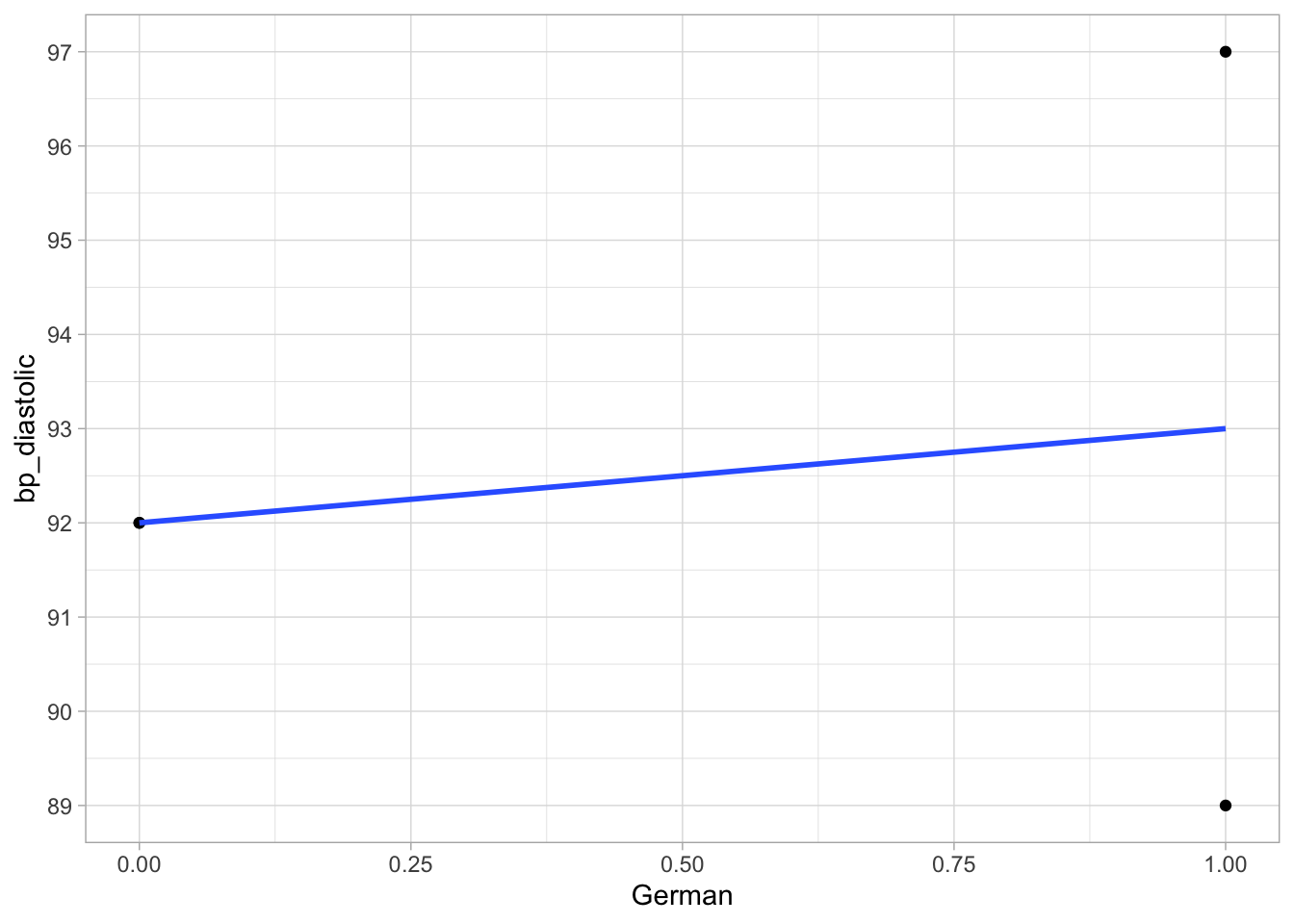
Figure 10.1: Linear regression of diastolic bloodpressure on the dummy variable German.
We learned that the slope in the model with such a dummy variable can be interpreted as the difference in the means for the two groups. In this case, the slope is equal to the difference in the means of the two groups in the sample data. The mean bloodpressure in the Dutch is \(\frac{92+92}{2}=\) 92 and in the Germans it is \(\frac{89+97}{2}=\) 93. The increase in mean bloodpressure if we move from German = 0 (Dutch) to German = 1 (German) is therefore equal to +1.
This is also what we see if R computes the regression for us, see Table 10.4.
| term | estimate | std.error | statistic | p.value |
|---|---|---|---|---|
| (Intercept) | 92 | 2.828 | 32.527 | 0.0009 |
| German | 1 | 4.000 | 0.250 | 0.8259 |
We see that being German has an effect of +1 units on the bloodpressure scale, with the individuals that are not German (Dutch) as the reference group. The intercept has the value 92 and that is the average bloodpressure in the non-German group. We can therefore view this +1 as the difference between mean German bloodpressure and mean Dutch bloodpressure.
Now suppose we do not have two groups, but three. We learned in Chapter 6 that we can have a hypothesis about the means of several groups. Suppose we have data from three groups, say Dutch, German and Italian. The data are in Table 10.5.
| participant | nationality | bp_diastolic |
|---|---|---|
| 1 | Dutch | 92 |
| 2 | German | 97 |
| 3 | German | 89 |
| 4 | Dutch | 92 |
| 5 | Italian | 91 |
| 6 | Italian | 96 |
When we run an ANOVA, the null hypothesis states that the means of the three groups are equal in the population. For example, the mean diastolic bloodpressure might be 92 for the Dutch, 93 for the Germans and 93.5 for the Italians, but this could result when the actual means in the population are the same: \(\mu_{Dutch}= \mu_{German}= \mu_{Italian}\).
If we would run an ANOVA we could get the following results
## Loading required package: carData##
## Attaching package: 'car'## The following object is masked from 'package:dplyr':
##
## recode## The following object is masked from 'package:purrr':
##
## someout <- bloodpressure %>%
lm(bp_diastolic ~ nationality, data = ., contrasts = list(nationality = contr.sum))
out %>%
Anova(type = 3) ## Anova Table (Type III tests)
##
## Response: bp_diastolic
## Sum Sq Df F value Pr(>F)
## (Intercept) 51708 1 3485.9438 1.07e-05 ***
## nationality 2 2 0.0787 0.9262
## Residuals 44 3
## ---
## Signif. codes: 0 '***' 0.001 '**' 0.01 '*' 0.05 '.' 0.1 ' ' 1We see an \(F\)-test with 2 and 3 degrees of freedom. The 2 results from the fact that we have three groups. This test is about the equality of the three group means. Compare this with the effects of the automatically created dummy variables in the lm() analysis below:
## # A tibble: 3 × 5
##   term               estimate std.error statistic   p.value
##   <chr>                 <dbl>     <dbl>     <dbl>     <dbl>
## 1 (Intercept)           92.0       2.72    33.8   0.0000570
## 2 nationalityGerman      1.00      3.85     0.260 0.812
## 3 nationalityItalian     1.50      3.85     0.389 0.723
In the output, the first \(t\)-test (33.8) is about the equality of the mean bloodpressure in the first group and 0. The second \(t\)-test (0.26) is about the equality of the means in groups 1 and 2, and the third \(t\)-test (0.389) is about the equality of the means in groups 1 and 3. The \(F\)-test from the ANOVA can be seen as a combination of two separate \(t\)-tests: the second and the third in this example, which are the ones about the equality of the last two group means and the first one. These two effects are from the two dummy variables created to code for the categorical variable nationality.
In the research you carry out, it is important to be clear on what you actually want to learn from the data. If you want to know if the data could have resulted from the situation where all population group means are equal, then the \(F\)-test is most appropriate. If you are more interested in whether the differences between certain countries and the first country (the reference country) are 0 in the population, the regular lm() table with the standard \(t\)-tests are more appropriate. If you are interested in other types of questions, then keep reading.
10.4 Contrasts and dummy coding
In the previous section we saw that when we run a linear model with a categorical predictor with two categories, we actually run a linear regression with a dummy variable. When the dummy variable codes for the category German, we see that the slope is the same as the mean of the German category minus the mean of the reference group. And we see that the intercept is the same as the mean of the reference group (the non-German group). We see that the dummy variable is 1 for Germans and 0 for Dutch, and that the use of this dummy variable in the analysis results in two parameters: (1) the intercept and (2) the slope. Actually these two parameters represent two contrasts. The first parameter contrasts the difference between the Dutch mean and 0 (again, the Dutch come first alphabetically and then the weight for the Germans):
\[L1 = M_{Dutch} = M_{Dutch} - 0 = 1 \times M_{Dutch} - 0 \times M_{German}\]
In the R output, this parameter (or contrast) is called ‘(Intercept)’. The second parameter contrasts the German mean with the Dutch mean:
\[L2 = M_{German} - M_{Dutch} = - 1 \times M_{Dutch} + 1 \times M_{German}\] This parameter is often denoted as the slope. In Table 10.4 above it is denoted as ‘German’.
These two contrasts can be represented in a contrast matrix containing two rows
\[\textbf{L} = \begin{bmatrix} 1 & 0 \\ -1 & 1 \end{bmatrix}\]
Suppose we want to have some different output. Suppose instead we want to see in the output the mean of the Germans first and then the extra bloodpressure in the Dutch. Earlier we learned that we can get that by using a dummy variable for being Dutch, so that the German group becomes the reference group. Here, we focus on the contrasts. Suppose we want the Germans to form the reference group, then we have to estimate the contrast:
\[L3: M_{German} = 0\times M_{Dutch} + 1 \times M_{German}\]
and then we can contrast the Dutch with this reference group:
\[L4: M_{Dutch} - M_{German} = 1 \times M_{Dutch} -1 \times M_{German}\] We then have the following contrast matrix:
\[\textbf{L} = \begin{bmatrix} 0 & 1 \\ 1 & -1 \end{bmatrix}\]
You see that when you make a choice regarding the dummy variable (either coding for being German or coding for being Dutch), this choice directly affects the contrasts that you make in the regression analysis (i.e., the output that you get). When using dummy variable German, the output gives contrasts \(L1\) and \(L2\), whereas using dummy variable Dutch leads to an output for contrasts \(L3\) and \(L4\).
To make this a bit more interesting, let’s look at a data example with three nationalities: Dutch, German and Italian. Suppose we want to use the German group as the reference group. We can then use the following contrast (the intercept):
\[L1: M_{German}\] Next, we are interested in the difference between the Dutch and this reference group:
\[L2 : M_{Dutch} - M_{German}\]
and the difference between the Italian and this reference group:
\[L3: M_{Italian} - M_{German}\] If we again order the three categories alphabetically, we can summarise these three contrasts with the contrast matrix
\[\textbf{L} = \begin{bmatrix} 0 & 1 & 0\\ 1 & -1 & 0 \\ 0 & -1 & 1 \end{bmatrix}\]
(please check this for yourself).
Based on what we learned from previous chapters, we know we can obtain these comparisons when we compute a dummy variable for being Dutch and a dummy variable for being Italian and use these in a linear regression. We see these dummy variables Dutch and Italian in Table 10.7.
| participant | nationality | Dutch | Italian | bp_diastolic |
|---|---|---|---|---|
| 1 | Dutch | 1 | 0 | 92 |
| 2 | German | 0 | 0 | 97 |
| 3 | German | 0 | 0 | 89 |
| 4 | Dutch | 1 | 0 | 92 |
| 5 | Italian | 0 | 1 | 91 |
| 6 | Italian | 0 | 1 | 96 |
This section showed that if you change the dummy coding, you change the contrasts that you are computing in the analysis. There exists a close connection between the contrasts and the actual dummy variables that are used in an analysis. We will discuss that in the next section.
10.5 Connection between contrast and coding schemes
We saw that what dummy coding you use determines the contrasts you get in the output of a linear model. In this section we discuss this intricate connection. As we saw earlier, the contrasts can be represented as a matrix \(\mathbf{L}\) with each row representing a contrast. Now let’s focus on the dummy coding. The way we code dummy variables, can be represented in a matrix \(\mathbf{S}\) where each column gives information about how to code a new numeric variable.
For a simple example, see the following matrix
\[\mathbf{S} =\begin{bmatrix} 1 & 0 \\ 0 & 1 \end{bmatrix}\]
Each row in this matrix represents a category: the first row is for the first category and the second row is for the second category. The columns represent the coding scheme for new variables. The first column specifies the coding scheme for the first new variable. The values are the values that should be used in constructing the new variables. The first column of \(\mathbf{S}\) specifies a dummy variable where the first category is coded as 1 and the second category as 0. The second column specifies the opposite: a dummy variable that codes the first category as 0 and the second category as 1.
If you want the short story for how (dummy) coding and contrasts are related: matrix \(\mathbf{S}\) (the coding scheme) is the inverse of the contrast matrix \(\mathbf{L}\). That is, if you have matrix \(\mathbf{L}\) and you want to know the coding scheme \(\mathbf{S}\), you can simply ask R to compute the inverse of \(\mathbf{L}\). This also goes the other way around: if you know what coding is used, you can take the inverse of the coding scheme to determine what the output represents. If you want to know what is meant with the inverse, see the advanced clickable section below, although it is not strictly necessary to know it. In order to work with linear models in R, it is sufficient to know how to compute the inverse in R.
A closer look at the \(\mathbf{L}\) and \(\mathbf{S}\) matrices and their connection
By default, R orders the categories of a factor alphabetically. If we have two groups, R uses by default the following coding scheme:
\[\textbf{S} = \begin{bmatrix} 1 & 0 \\ 1 & 1 \end{bmatrix}\]
This matrix has two rows and two columns. Each row represents a category. In our earlier example, the first category is “Dutch” and the second category is “German” (categories sorted alphabetically). Each column of the matrix \(\mathbf{S}\) represents a new numeric variable that R will compute in order to code for the categorical factor variable. The first column (representing a new numeric variable) says that for both categories (rows), the new variable gets the value 1. The second column holds a 0 and a 1. It says that the first category is coded as 0, and the second category is coded as 1.
Thus, this matrix says that we should create two new variables. They are displayed in Table 10.9, where we call them Intercept and German, respectively. Why we name the second new variable German is obvious: it’s simply a dummy variable for coding “German” as 1. Why we call the first variable Intercept is less obvious, but we will come back to that later.
Thus, with matrix \(\mathbf{S}\), you have all the information you need to perform a linear regression analysis with only numerical variables.
With matrix \(\mathbf{S}\) as the default, what kind of contrasts will we get, and how can we find out? It turns out that once you know \(\mathbf{S}\), you can immediately calculate (or have R calculate) what kind of contrast matrix \(\mathbf{L}\) you get. The connection between matrices \(\mathbf{L}\) and \(\mathbf{S}\) is the same as the connection between 4 and \(\frac{1}{4}\).
You might know that \(\frac{1}{4}\) is called the reciprocal of 4. The reciprocal of 4 can also be denoted by \(4^{-1}\). Thus we can write that the reciprocal of 4 is as follows:
\[4^{-1} = \frac{1}{4}\]
We can say that if we have a quantity \(x\), the reciprocal of \(x\) is defined as that number when multiplied with \(x\), results in 1.
\[x x^{-1} = x^{-1} x = 1\]
Examples
- The reciprocal of 3 is equal to \(\frac{1}{3}\), because \(3 \times \frac{1}{3} = 1\).
- The reciprocal of \(\frac{1}{100}\) is equal to 100, because \(\frac{1}{100} \times 100 = 1\).
- The reciprocal of \(\frac{3}{4}\) is equal to \(\frac{4}{3}\), because \(\frac{3}{4}\times \frac{4}{3} = 1\).
Just like a number has a reciprocal, a matrix has an inverse. Similar to reciprocals, we use the “-1” to indicate the inverse of a matrix. We have that by definition, \(\mathbf{L}\mathbf{L}^{-1}=\mathbf{I}\) and \(\mathbf{S}\mathbf{S}^{-1}=\mathbf{I}\), where matrix \(\mathbf{I}\) is the matrix analogue of a 1, and its called an identity matrix. It turns out that the inverse of matrix \(\mathbf{L}\) is \(\mathbf{S}\): \(\mathbf{L}^{-1}=\mathbf{S}\), and the inverse of \(\mathbf{S}\) equals \(\mathbf{L}\): \(\mathbf{S}^{-1}=\mathbf{L}\). That implies we have that \(\mathbf{L} \mathbf{S} = \mathbf{I}\). The only difference with reciprocals is that \(\mathbf{L}\) and \(\mathbf{S}\) are matrices, so that we are in fact performing matrix algebra, which is a little bit different from algebra with single numbers. Nevertheless, it is true that if we matrix multiply \(\mathbf{L}\) and \(\mathbf{S}\), we get a matrix \(\mathbf{I}\). This matrix is as we said an identity matrix, which means it has only 1s on the diagonal (from top-left to bottom-right) and 0s elsewhere:
\[\mathbf{L}\mathbf{S} = \mathbf{S}\mathbf{L} = \mathbf{I} = \begin{bmatrix} 1 & 0 \\ 0 & 1 \end{bmatrix}\]
It turns out that if we have \(\mathbf{S}\) as defined above (the default coding scheme), the contrast matrix \(\mathbf{L}\) can only be
\[\mathbf{L} = \begin{bmatrix} 1 & 0 \\ -1 & 1 \end{bmatrix}\]
or written in full:
\[\mathbf{S}\mathbf{L} = \begin{bmatrix} 1 & 0 \\ 1 & 1 \end{bmatrix} \times \begin{bmatrix} 1 & 0 \\ -1 & 1 \end{bmatrix} = \begin{bmatrix} 1 & 0 \\ 0 & 1 \end{bmatrix}\]
Please note that you don’t have to know matrix algebra when studying this book, but it helps to understand what is going on when performing linear regression analysis with categorical variables. By having R do the matrix algebra for you, you can fully control what kind of output you want from an analysis.
| participant | nationality | Intercept | German | bp_diastolic |
|---|---|---|---|---|
| 1 | Dutch | 1 | 0 | 92 |
| 2 | German | 1 | 1 | 97 |
| 3 | German | 1 | 1 | 89 |
| 4 | Dutch | 1 | 0 | 92 |
10.6 Working with matrices \(\mathbf{S}\) and \(\mathbf{L}\) in R
In the last section we saw that coding scheme matrix \(\mathbf{S}\) is the inverse of contrast matrix \(\mathbf{L}\), and contrast matrix \(\mathbf{L}\) is the inverse of coding scheme matrix \(\mathbf{S}\). In this section we see how to compute the inverse of a matrix R.
Let’s take the bloodpressure example again, where we had data on three nationalities: in alphabetical order the Dutch data, then the German data, and lastly the Italian data.
Let’s assume we want to use the German group as the reference group. We then need a matrix \(\mathbf{L}\) similar to the one from a previous section with the nationalities Dutch, German and Italian (in alphabetical order), with German as the reference category (the second group). We enter that contrast matrix \(\mathbf{L}\) in R as follows:
##      [,1] [,2] [,3]
## [1,]    0    1    0
## [2,]    1   -1    0
## [3,]    0   -1    1
The first row is the contrast for the mean of the second group (German). The second row contrasts the first group (Dutch) with the second group (German). The third row contrasts the third group (Italian) with the second group (German).
If we are interested in the coding scheme matrix, we take the inverse of \(\mathbf{L}\) to get matrix \(\mathbf{S}\) by using the ginv() function, that is available in the package MASS.
library(MASS)
S <- ginv(L)  # S is calculated as the inverse of L
S %>% fractions() # to get more readable output
## [,1] [,2] [,3]
## [1,] 1 1 0
## [2,] 1 0 0
## [3,] 1 0 1The output is a coding scheme matrix with 3 columns:
\[\textbf{S} = \begin{bmatrix} 1 & 1 & 0\\ 1 & 0 & 0 \\ 1 & 0 & 1 \end{bmatrix}\]
This coding scheme matrix \(\mathbf{S}\) tells us what kind of variables to compute to obtain these contrasts in \(\mathbf{L}\) in the output of the linear model. Each column of \(\mathbf{S}\) contains the information for each new variable. Since we have three columns, we know that we need to compute three variables. The first column tells us that the first variable consists of the value 1 for all groups. We will come back to this variable of 1s later (it represents the intercept). The second column indicates we need a dummy variable that codes the first group (Dutch) as 1 and the other two groups as 0. The third column tells us we need a third variable that is also a dummy variable, coding 1 for group 3 (Italian) and 0 for the other two groups.
If we apply this coding scheme to our data set, then we get the following data matrix:
| participant | nationality | bp_diastolic | v1 | v2 | v3 |
|---|---|---|---|---|---|
| 1 | Dutch | 92 | 1 | 1 | 0 |
| 2 | German | 97 | 1 | 0 | 0 |
| 3 | German | 89 | 1 | 0 | 0 |
| 4 | Dutch | 92 | 1 | 1 | 0 |
| 5 | Italian | 91 | 1 | 0 | 1 |
| 6 | Italian | 96 | 1 | 0 | 1 |
Now let’s do the exercise the other way around. If you know the coding scheme (how your dummy variables are coded), you can easily determine what the output will represent. For instance, let \(\mathbf{S}\) be the coding scheme for a dummy variable for group 1 (Dutch) and a dummy variable for group 2 (German) (with reference group “Italian”). We enter that in R:
By default, any lm() analysis includes an intercept, and an intercept is always coded as 1. We therefore add a variable of only 1s to represent the intercept (why these 1s are included will become clear).
##      [,1] [,2] [,3]
## [1,]    1    1    0
## [2,]    1    0    1
## [3,]    1    0    0
We can then determine what contrasts these three variables will lead to by taking the inverse to calculate contrast matrix \(\mathbf{L}\):
##      [,1] [,2] [,3]
## [1,]  0    0    1
## [2,]  1    0   -1
## [3,]  0    1   -1
This matrix \(\mathbf{L}\) contains three rows, one for each contrast. The first row gives a contrast \(L1\) which is \(0 \times M_1 + 0 \times M_2 + 1 \times M_3\) which is equal to \(M_3\) (the Italian mean). The second row gives contrast \(1\times M_1 + 0 \times M_2 - 1\times M_3\) which amounts to the first group mean minus the last one, \(M_1 - M_3\) (difference between Dutch and Italian). The third row gives the contrast \(0\times M_1 + 1 \times M_2 - 1\times M_3\) which is \(M_2 - M_3\) (difference between German and Italian).
Remember, contrast matrix \(\mathbf{L}\) is organised in rows, whereas coding scheme matrix \(\mathbf{S}\) is organised in columns. One way to memorise this is to realise that coding scheme matrix \(\mathbf{S}\) defines new variables, and variables are organised as columns in a data matrix, as you may recall from Chapter 1.
You may wonder, what is this variable with only 1s doing in this story? Didn’t we learn that we only need to compute 2 dummy variables for a categorical variable with 3 categories? The short answer is: the variable with only 1s (for all categories) represents the intercept, which is always included in a linear model by default. For more explanation, click on the link below.
A closer look at the intercept represented as a variable with 1s
In most regression analyses, we want to include an intercept in the linear model. This happens so often that we forget that we have a choice here. For instance, in R, an intercept is included by default. For example, if you use the code with the formula bp_diastolic ~ nationality, you get the exact same result as with bp_diastolic ~ 1 + nationality. In other words, by default, R computes a variable that consists of only 1s. This can be seen if we use the model.matrix() function. This function shows the actual variables that are computed by R and used in the analysis.
##   (Intercept) nationalityGerman nationalityItalian
## 1           1                 0                  0
## 2           1                 1                  0
## 3           1                 1                  0
## 4           1                 0                  0
## 5           1                 0                  1
## 6           1                 0                  1
## attr(,"assign")
## [1] 0 1 1
## attr(,"contrasts")
## attr(,"contrasts")$nationality
## [1] "contr.treatment"
In the output, we see the actual numeric variables that are used in the analysis for the six observations in the data set (six rows). Taken together, these variables, displayed as columns in a matrix, are called the design matrix.
We see a variable called (Intercept) with only 1s and two dummy variables, one coding for Germans, with the name nationalityGerman, and one coding for Italians with the name nationalityItalian. These variable names we see again when we look at the results of the lm() analysis:
## # A tibble: 3 × 5
##   term               estimate std.error statistic   p.value
##   <chr>                 <dbl>     <dbl>     <dbl>     <dbl>
## 1 (Intercept)           92.0       2.72    33.8   0.0000570
## 2 nationalityGerman      1.00      3.85     0.260 0.812
## 3 nationalityItalian     1.50      3.85     0.389 0.723
Now the names of the newly computed variables have become the names of parameters (the intercept and slope parameters). These parameter values actually represent the (default) contrasts \(L1\), \(L2\) and \(L3\), here quantified as 92.0, 1.0 and 1.5, respectively. The ‘intercept’ of 92.0 is simply the quantity that we find for the first contrast (the first row in the contrast matrix \(\mathbf{L}\)).
In summary, when you have three groups, you can invent a quantitative variable called (intercept) that is equal to 1 for all observations in your data matrix. If you then also invent a dummy variable for being German and a dummy variable for being Italian, and submit these three variables to a linear model analysis, the output will yield the mean of the Dutch, the difference between the German mean and the Dutch mean, and the difference between the Italian mean and the Dutch mean. In the code below, you see what is actually going on: the computation of the three variables and submitting these three variables to an lm() analysis. Note that R by default includes an intercept. To suppress this behaviour, we include -1 in the formula:
dummy_German   <- c(0, 1, 1, 0, 0, 0)
dummy_Italian  <- c(0, 0, 0, 0, 1, 1)
iNtErCePt      <- c(1, 1, 1, 1, 1, 1)
bp_diastolic   <- c(92, 97, 89, 92, 91, 96)

lm(bp_diastolic ~ iNtErCePt + dummy_German + dummy_Italian - 1) %>%
  tidy()
## # A tibble: 3 × 5
## term estimate std.error statistic p.value
## <chr> <dbl> <dbl> <dbl> <dbl>
## 1 iNtErCePt 92.0 2.72 33.8 0.0000570
## 2 dummy_German 1.00 3.85 0.260 0.812
## 3 dummy_Italian 1.50 3.85 0.389 0.723You see that you get the exact same results as in the default way, by specifying a categorical variable nationality:
nationality <- factor(c(1, 2, 2, 1, 3,3 ),
                      labels = c("Dutch", "German", "Italian"))

lm(bp_diastolic ~ nationality) %>%
  tidy()
## # A tibble: 3 × 5
## term estimate std.error statistic p.value
## <chr> <dbl> <dbl> <dbl> <dbl>
## 1 (Intercept) 92.0 2.72 33.8 0.0000570
## 2 nationalityGerman 1.00 3.85 0.260 0.812
## 3 nationalityItalian 1.50 3.85 0.389 0.723Or when doing the dummy coding yourself:
## # A tibble: 3 × 5
## term estimate std.error statistic p.value
## <chr> <dbl> <dbl> <dbl> <dbl>
## 1 (Intercept) 92.0 2.72 33.8 0.0000570
## 2 dummy_German 1.00 3.85 0.260 0.812
## 3 dummy_Italian 1.50 3.85 0.389 0.723and in a way where we explicitly include an intercept of 1s:
## # A tibble: 3 × 5
##   term               estimate std.error statistic   p.value
##   <chr>                 <dbl>     <dbl>     <dbl>     <dbl>
## 1 (Intercept)           92.0       2.72    33.8   0.0000570
## 2 nationalityGerman      1.00      3.85     0.260 0.812
## 3 nationalityItalian 1.50 3.85 0.389 0.723## # A tibble: 3 × 5
## term estimate std.error statistic p.value
## <chr> <dbl> <dbl> <dbl> <dbl>
## 1 (Intercept) 92.0 2.72 33.8 0.0000570
## 2 dummy_German 1.00 3.85 0.260 0.812
## 3 dummy_Italian 1.50 3.85 0.389 0.723with the only difference that the first parameter is now called ‘(Intercept)’.
In conclusion: linear models by default include an ‘intercept’ that is actually coded as an independent variable consisting of all 1s.
10.7 Choosing the reference group in R for dummy coding
Let’s see how to run an analysis in R, when we want to control what contrasts are actually computed. This time, we want to let the Germans form the reference group, and then compare the Dutch and Italian means with the German mean.
Let’s first put the data from Table 10.5 in R, so that you can follow along using your own computer (copy the code below into an R-script).
# create a dataframe (a tibble is the tidyverse version of a dataframe)
bloodpressure <- tibble(
  participant = c(1, 2, 3, 4, 5, 6),
  nationality = c("Dutch", "German", "German", "Dutch", "Italian", "Italian"),
  bp_diastolic = c(92, 97, 89, 92, 91, 96))
bloodpressure
## # A tibble: 6 × 3
## participant nationality bp_diastolic
## <dbl> <chr> <dbl>
## 1 1 Dutch 92
## 2 2 German 97
## 3 3 German 89
## 4 4 Dutch 92
## 5 5 Italian 91
## 6 6 Italian 96Note that we omit dummy variables for now. Next we turn the nationality variable in the tibble bloodpressure into a factor variable. This ensures that R knows that it is a categorical variable.
If we then look at this factor,
## [1] Dutch   German  German  Dutch   Italian Italian
## Levels: Dutch German Italian
we see that it has three levels. With the levels() function, we see that the first level is Dutch, the second level is German, and the third level is Italian. This is default behaviour: R chooses the order alphabetically.
## [1] "Dutch" "German" "Italian"This means that if we run a standard lm() analysis, the first level (the Dutch) will form the reference group, and that the two slope parameters stand for the contrasts of the bloodpressure in Germans and Italians versus the Dutch, respectively:
##
## Call:
## lm(formula = bp_diastolic ~ nationality, data = .)
##
## Coefficients:
##        (Intercept)   nationalityGerman  nationalityItalian
##               92.0                 1.0                 1.5
In the case that we want to use the Germans as the reference group instead of the Dutch, we have to specify a set of contrasts that is different from this default set of contrasts.
One way to easily do this is to permanently set the reference group to another level of the nationality variable. We work with the variable nationality in the dataframe (or tibble) called bloodpressure. We use the relevel() function to change the reference group to “German”.
If we check this by using the function levels() again, we see that the first group is now German, and no longer Dutch:
## [1] "German" "Dutch" "Italian"If we run an lm() analysis, we see from the output that the reference group is now indeed the German group (i.e., with contrasts for being Dutch and Italian).
##
## Call:
## lm(formula = bp_diastolic ~ nationality, data = .)
##
## Coefficients:
##        (Intercept)    nationalityDutch  nationalityItalian
##               93.0                -1.0                 0.5
To check this fully, we can ask R to show us the dummy variables that it created for the analysis, using the function model.matrix().
##   (Intercept) nationalityDutch nationalityItalian
## 1           1                1                  0
## 2           1                0                  0
## 3           1                0                  0
## 4           1                1                  0
## 5           1                0                  1
## 6           1                0                  1
## attr(,"assign")
## [1] 0 1 1
## attr(,"contrasts")
## attr(,"contrasts")$nationality
## [1] "contr.treatment"
The output gives the values for the new variables for all individuals in the original dataset. We see that R created a dummy variable for being Dutch (named nationalityDutch), and another dummy variable for being Italian (named nationalityItalian). Therefore, the reference group is now formed by the Germans. Note that R also created a variable called (Intercept), that consists of only 1s for all six individuals.
The variable nationality in the dataframe bloodpressure is now permanently altered. From now on, every time we use this variable in an analysis, the reference group will be formed by the Germans. By using mutate() and relevel() again, we can change everything back or pick another reference group.
This fixing of the reference category is very helpful in data analysis for experimental data. Suppose a researcher wants to quantify the effects of vaccine A and vaccine B on hospitalisation for COVID-19. She randomly assigns individuals to one of three groups: A, B and C, where group C is the control condition in which individuals receive a saline injection (placebo). Individuals in group A and group B get vaccines A and B, respectively. In order to quantify the effect of vaccine A, you would like to contrast group A with group C, and in order to quantify the effect of vaccine B, you would like to contrast group B with group C. In that case, it is helpful if the reference group is group C. By default, R uses the first category as the reference category, when ordered alphabetically. By default therefore, R would choose group A as the reference group. R would then by default compute the contrast between B and A, and between C and A, apart from the mean of group A (the intercept). By changing the reference category to group C, the output would be more helpful to answer the research question.
Summary
General steps to take for using dummy coding and choosing the reference category:
- Use
levels()to check what group is named first. That group will generally be the reference group. For example, dolevels(data$variable). - If the reference group is not the right one, use
mutate()andrelevel()to change the reference group, for example do something like:data <- data %>% mutate(variable = relevel(variable, ref = "German")). - Verify with
levels()whether the right reference category is now mentioned first. Any new analysis usinglm()will now yield an analysis with dummy variables for all categories except the first one.
10.8 Alternative coding schemes
By default, R uses dummy coding. Contrasts that are computed by using dummy variables are called treatment contrasts: these contrasts are the difference between the individual groups and the reference group. Similar to defining the reference group for a particular variable (so that the first parameter value in the output is the mean of this reference group, usually termed (Intercept)), you can set all contrasts that are used in the linear model analysis. For instance by typing
##         Dutch Italian
## German      0       0
## Dutch       1       0
## Italian     0       1
you see that the first variable that is created (the first column) is a dummy variable for being Dutch, and the second variable is a dummy for being Italian. What you see in the contrasts() matrix is not the contrasts per se, but the coding scheme for the new variables that are created by R. In other words, with contrasts() you get to see the coding scheme matrix \(\mathbf{S}\). Note however that the default variable with 1s (the intercept) is not displayed.
This default treatment coding (dummy coding) is fine for linear regression, but not so great for ANOVAs. We will come back to this issue in a later section when discussing moderation. For now it suffices to know that if you are interested in an ANOVA rather than a linear regression analysis, it is best to use effects coding (sometimes called sum-to-zero contrasts). Above we saw that the first column after the contrasts() function (called ‘Dutch’) sums to 1, and the second column (called ‘Italian’) also sums to 1. In effects coding on the other hand, the weights for each contrast sum to 0 (hence the name sum-to-zero contrasts). Effects coding is also useful if we have specific research questions where we are interested in differences between combinations of groups. We will see in a moment what that means. Below we discuss effects coding in more detail, and also discuss other standard ways of coding (Helmert contrasts and successive differences contrast coding).
10.8.1 Effects coding
Below we will illustrate how to use and interpret a linear model when we apply effects coding. You can type along in R.
First, let’s check that we have everything in the original alphabetical order. This makes it easier to not get distracted by details.
## [1] "German" "Dutch" "Italian"# change the order such that "Dutch" becomes the first group
bloodpressure <- bloodpressure %>%
mutate(nationality = relevel(nationality, ref = "Dutch"))
bloodpressure$nationality %>%
levels() # Check that Dutch is now the first group## [1] "Dutch" "German" "Italian"Next, we need to change the default dummy coding into effects coding for the nationality variable in the bloodpressure dataframe. We do that by again fixing something permanently for this variable. We use the function code_deviation() from the codingMatrices package.
library(codingMatrices) # install if not already done
contrasts(bloodpressure$nationality) <- code_deviation
When we run contrasts() again, we see a different set of columns, where each column now sums to 0. We no longer see dummy coding.
##         MD1 MD2
## Dutch     1   0
## German    0   1
## Italian  -1  -1
The values in this coding scheme matrix are used to code for the new numeric variables. The first column says that a variable should be created with 1s for Dutch, 0s for Germans and -1s for Italians. The second column indicates that another variable should be created with 0s for Dutch, 1s for Germans and -1s for Italians. Any new analysis with the variable nationality in the dataframe bloodpressure will now by default use this sum-to-zero coding scheme. If we run a linear model analysis with this factor variable, we see that we get very different values for the parameters.
## # A tibble: 3 × 5
##   term           estimate std.error statistic   p.value
##   <chr>             <dbl>     <dbl>     <dbl>     <dbl>
## 1 (Intercept)      92.8        1.57   59.0    0.0000107
## 2 nationalityMD1   -0.833      2.22   -0.375  0.733
## 3 nationalityMD2    0.167      2.22    0.0750 0.945
Let’s check that we understand how the new variables are computed.
##   (Intercept) nationalityMD1 nationalityMD2
## 1           1              1              0
## 2           1              0              1
## 3           1              0              1
## 4           1              1              0
## 5           1             -1             -1
## 6           1             -1             -1
## attr(,"assign")
## [1] 0 1 1
## attr(,"contrasts")
## attr(,"contrasts")$nationality
##         MD1 MD2
## Dutch     1   0
## German    0   1
## Italian  -1  -1
We still have a variable called (Intercept) with only 1s, which is used by default, as we saw earlier. There are also two other new variables, one called nationalityMD1 and the other called nationalityMD2, where there are 1s, 0s and -1s.
Based on this coding scheme it is hard to say what the new values in the output represent. But we saw earlier that the output values are simply the values for the contrasts, and the contrasts can be determined by taking the inverse of the coding scheme matrix \(\mathbf{S}\).
Matrix \(\mathbf{S}\) consists now of the effects coding scheme. \(\mathbf{S}\) is therefore the same as the output of contrasts(bloodpressure$nationality).
##         MD1 MD2
## Dutch     1   0
## German    0   1
## Italian  -1  -1
We see that it has the two new numeric variables. We miss however the variable with 1s that is used by default in the analysis. If we add that we get the full matrix \(\mathbf{S}\) with the three new variables.
##           MD1 MD2
## Dutch   1   1   0
## German  1   0   1
## Italian 1  -1  -1
Next we take the inverse to compute contrast matrix \(\mathbf{L}\).
## [,1] [,2] [,3]
## [1,] 0.3333333 0.3333333 0.3333333
## [2,] 0.6666667 -0.3333333 -0.3333333
## [3,] -0.3333333 0.6666667 -0.3333333## [,1] [,2] [,3]
## [1,] 1/3 1/3 1/3
## [2,] 2/3 -1/3 -1/3
## [3,] -1/3 2/3 -1/3This gives us what we need to know about how to interpret the output. Briefly, the first parameter in the output now represents what is called the grand mean. This is the mean of all group means. This is so, because if we put the group means in the right order, and we use the weights from the first row in \(\mathbf{L}\), we get
\[L1: \frac{1}{3} M_{Dutch} + \frac{1}{3} M_{German} + \frac{1}{3} M_{Italian}\] which can be simplified to
\[L1: \frac{ M_{Dutch} + M_{German} + M_{Italian}}{3}\] which is the mean of the three group means. We generally call the mean of group means the grand mean.
For the meaning of the second parameter we look at the second row of the contrast matrix and fill in the numbers for a second contrast:
\[L2: \frac{2}{3} M_{Dutch} - \frac{1}{3} M_{German} - \frac{1}{3} M_{Italian}\]
\(L2\) can be rewritten as
\[L2: \frac{2}{3} \times \large(M_{Dutch} - \frac{ M_{German} + M_{Italian}}{2}\large)\] \(L2\) is therefore the difference between the Dutch mean and the mean of the other two means, multiplied by \(\frac{2}{3}\).
Although it makes sense to interpret this contrast as the difference between the Dutch mean and the other two means, the fraction \(\frac{2}{3}\) looks weird here. Let’s therefore rewrite contrast \(L2\) in a different way:
\[\begin{aligned} L2&: \frac{2}{3} M_{Dutch} - \frac{1}{3} M_{German} - \frac{1}{3} M_{Italian} \\ &= \frac{2}{3} M_{Dutch} + \frac{1}{3} M_{Dutch} - \frac{1}{3} M_{Dutch} - \frac{1}{3} M_{German} - \frac{1}{3} M_{Italian}\\ &= M_{Dutch} - \frac{ M_{Dutch} + M_{German} + M_{Italian}}{3}\end{aligned}\]
In other words, this contrast is about the difference between the Dutch mean and the grand mean.
For the meaning of the third parameter we look at the third row of the contrast matrix and fill in the numbers for a second contrast:
\[L3: -\frac{1}{3} M_{Dutch} + \frac{2}{3} M_{German} - \frac{1}{3} M_{Italian}\] which can be written as
\[L3: \frac{2}{3} \times \large(M_{German} - \frac{ M_{Dutch} + M_{Italian}}{2}\large)\]
and interpreted as the difference between the German mean and the mean of the other two means, multiplied by \(\frac{2}{3}\), or, when writing it out like
\[L3: M_{German} - \frac{ M_{Dutch} + M_{German} + M_{Italian}}{3}\]
as the difference between the German mean and the grand mean.
Let’s check whether this makes sense. Let’s get an overview of the group means in the data, and the coefficients again:
## # A tibble: 3 × 2
## nationality mean
## <fct> <dbl>
## 1 Dutch 92
## 2 German 93
## 3 Italian 93.5## (Intercept) nationalityMD1 nationalityMD2
## 92.8333333 -0.8333333 0.1666667The first parameter ‘(Intercept)’ equals 92.833 and this is indeed equal to the grand mean \(\frac{(92 + 93 + 93.5)}{3} = 92.833\).
The second parameter ‘nationalityMD1’ equals -0.833 and this is equal to the difference between the Dutch mean 92 and the German and Italian means combined, \(\frac{(93 + 93.5)}{2} = 93.25\), so \(92 - 93.25 = -1.25\). When we multiply this by \(\frac{2}{3}\), we get \(-1.25 \times \frac{2}{3} = -0.833\).
The third parameter ‘nationalityMD2’ equals 0.167 and this is indeed equal to the difference between the German mean 93 and the Dutch and Italian means combined, \(\frac{(92 + 93.5)}{2} = 92.75\), so \(93 - 92.75 = 0.25\). When multiplied by \(\frac{2}{3}\), we get \(0.25 \times \frac{2}{3} = 0.167\). This multiplication is explained in more detail below.
It also computes when we define the contrasts in terms of the grand mean. Let’s first compute the grand mean (the mean of all three means):
bloodpressure %>%
group_by(nationality) %>%
summarise(mean = mean(bp_diastolic)) %>% # the group means
summarise(grandmean = mean(mean)) # compute mean of the group means## # A tibble: 1 × 1
## grandmean
## <dbl>
## 1 92.8and compare it to the group means:
## # A tibble: 3 × 2
## nationality mean
## <fct> <dbl>
## 1 Dutch 92
## 2 German 93
## 3 Italian 93.5We see that \(L2\) should be \(92 - 92.8 = -0.8\), and that \(L3\) should be \(93 - 92.8 = 0.2\), which is exactly what we find as coefficients in the output (safe rounding).
## (Intercept) nationalityMD1 nationalityMD2
## 92.8333333 -0.8333333 0.1666667Effects coding is interesting in all cases where you want to test a null-hypothesis about one group versus the mean of the other groups (or versus the grand mean). As we saw above, the second parameter in the output is about the difference between the first group mean and the average of all group means (the grand mean). The \(t\)-test that goes along with that parameter informs us about the null-hypothesis that the first group has the same population mean as the average of all the other group means (in other words, that the group mean is the same as the grand mean). This is useful in a situation where you for example want to compare the control/placebo condition with several experimental conditions combined: do the various treatments in general result in a different mean than when doing nothing?
Suppose for example that we do a study on various types of therapy to quit smoking. In one group, people are put on a waiting list, in a second group people receive treatment using nicotine patches and in a third group, people receive treatment using cognitive behavioural therapy.
If your main questions are (1) what is the effect of nicotine patches on the number of cigarettes smoked, and (2) what is the effect of cognitive behavioural therapy on number of cigarettes smoked, you may want to go for the default dummy coding strategy and make sure that the control condition is the first level of your factor. The parameters and the \(t\)-tests that are relevant for your research questions are then in the second and third row of your regression table.
However, if your main question is: “Do treatments like nicotine patches and cognitive behavioural therapy help reduce the number of cigarettes smoked, compared to doing nothing?” you might want to opt for a sum-to-zero (effects coding) strategy, where you make sure that the control condition (waiting list) is the first level of your factor. The relevant null-hypothesis test for your research question is then given in the second line of your regression table (contrasting the control group with the two treatments groups, i.e., contrasting the control group with the grand mean).
Summarising, there are multiple ways of carrying out a linear model analysis with categorical variables. The R default way is to use dummy coding, and the second way is effects coding. Unless you are particularly interested in an ANOVA with multiple independent categorical variables, or about combinations of groups, the default way with dummy coding is just fine. Regarding ANOVA, most software packages and functions that perform ANOVA actually use effects coding by default, so it is important to be familiar with it. It must be said however, that ANOVA results for analyses with one independent variable will not be affected by using a different coding scheme. The coding scheme underlying an ANOVA only matters as soon as you have multiple independent variables.
In previous chapters we learned how to read the output from an lm() analysis when it is based on dummy coding. In the current subsection we saw how to figure out what the numbers in the output represent in case of effects coding. Now we will look at a number of other alternatives of coding categorical variables, after which we will look into how to make user-specified contrasts, that help you answer your own particular research question.
10.8.2 Helmert contrasts
One other well-known coding scheme is a Helmert coding scheme. We can specify we want Helmert contrasts for the nationality variable if we code the following
contrasts(bloodpressure$nationality) <- code_helmert
contrasts(bloodpressure$nationality) %>% fractions()## H2 H3
## Dutch -1/2 -1/3
## German 1/2 -1/3
## Italian 0 2/3The first column indicates how the first new variable is coded (Dutch as \(-\frac{1}{2}\), Germans as \(\frac{1}{2}\) and Italians as 0), and the second column indicates a new variable with \(-\frac{1}{3}\) for Germans and Dutch, and \(\frac{2}{3}\) for Italians. By default another variable is computed as 1s for all groups, representing some kind of intercept.
If we do the same trick to this matrix as before, by adding a column of 1s and then using ginv(), we get the following weights for the contrasts that we are quantifying this way
## [,1] [,2] [,3]
## [1,] 1/3 1/3 1/3
## [2,] -1 1 0
## [3,] -1/2 -1/2 1Again each row gives the weights for the contrasts that are computed. Similar as with effects coding, the first contrast represents the grand mean (the mean of the group means):
\[L1: \frac{M_{Dutch} + M_{German} + M_{Italian}}{3}\]
The second row represents the difference between German and Dutch means:
\[L2: - 1 \times M_{Dutch} + 1 \times M_{German} + 0 \times M_{Italian}= M_{German} - M_{Dutch}\]
and the third row represents the difference between the Italian mean on the one hand, and the Dutch and German means combined.
\[ -\frac{1}{2} \times M_{Dutch} - \frac{1}{2} \times M_{German} + 1 \times M_{Italian} = M_{Italian} - \frac{M_{Dutch} + M_{German}}{2}\] In general, with a Helmert coding scheme (1) the first group is compared to the second group, (2) the first and second group combined is compared to the third group, (3) the first, second and third group combined is compared to the fourth group, and so on. Let’s imagine we have a country factor variable with five levels. Let’s then indicate that we want to have Helmert contrasts.
country <- c("A", "B", "C", "D", "E") %>% as.factor()
contrasts(country) <- code_helmert
contrasts(country)## H2 H3 H4 H5
## A -0.5 -0.3333333 -0.25 -0.2
## B 0.5 -0.3333333 -0.25 -0.2
## C 0.0 0.6666667 -0.25 -0.2
## D 0.0 0.0000000 0.75 -0.2
## E 0.0 0.0000000 0.00 0.8then we do the trick to get the rows with the contrasts weights
## [,1] [,2] [,3] [,4] [,5]
## [1,] 1/5 1/5 1/5 1/5 1/5
## [2,] -1 1 0 0 0
## [3,] -1/2 -1/2 1 0 0
## [4,] -1/3 -1/3 -1/3 1 0
## [5,] -1/4 -1/4 -1/4 -1/4 1Then we see that the first contrast is the general mean. The second row is a comparison between A and B, the third one a comparison between (A+B)/2 and C, the fourth one a comparison between (A+B+C)/3 and D, and the fifth one a comparison between (A+B+C+D)/4 with E. To put it differently, the Helmert contrasts compare each level with the average of the ‘preceding’ levels. Thus, we can compare categories of a variable with the mean of the preceding categories of the variable.
You can also choose to go the other way around. If we use the function code_helmert_forward instead of code_helmert
contrasts(country) <- code_helmert_forward
S <- cbind(1, contrasts(country))
L <- ginv(S)
L %>% fractions() # to make it easier to read## [,1] [,2] [,3] [,4] [,5]
## [1,] 1/5 1/5 1/5 1/5 1/5
## [2,] 1 -1/4 -1/4 -1/4 -1/4
## [3,] 0 1 -1/3 -1/3 -1/3
## [4,] 0 0 1 -1/2 -1/2
## [5,] 0 0 0 1 -1you see that we go ‘forward’: after the general mean, we see that country A is compared to (B+C+D+E)/4, then country B is compared to (C+D+E)/3; next, country C is compared to (D + E)/2 and lastly D is compared to E. This forward type of Helmert coding is usually the default Helmert coding in other statistical packages.
Helmert contrasts are useful when you have a particular logic for ordering the levels of a categorical variable (i.e. if you have an ordinal variable). An example where a Helmert contrast might be useful is when you want to know the minimal effective dose in a dose-response study. Suppose we have a new medicine and we want to know how much of it is needed to end a headache. We split individuals with headache into four groups. In group A, people take a placebo pill, in group B people take 1 tablet of the new medicine, in group C people take 3 tablets, and in group D people take 4 tablets. In the data analysis, we first want to establish whether 1 tablet leads to a significant reduction compared to placebo. If that is not the case, we can test whether 3 tablets (group C) work better than either 1 tablet or no tablet (groups A and B combined). If that doesn’t show a significant improvement either, we may want to compare 6 tablets (group D) versus fewer tablets (groups A, B and C combined).
There are a couple of other standard options in R for coding your variables. Successive differences contrast coding is also an option for meaningfully ordered categories. It compares the second level with the first level, the third level with the second level, the fourth level with the third level, and so on. The function to be used is code_diff (available in the codingMatrices package). It could be a useful alternative to Helmert coding for a dose-response study. Other alternatives are given in Table 10.14.
| option | description |
|---|---|
| code_control | For contrasts that compare the group means (the ‘treatments’) with the first class mean (the reference group). |
| code_control_last | Similar to ‘code_control’, but using the final class mean as the reference group |
| code_diff | The contrasts are the successive differences of the treatment means, e.g. group 2 - group 1, group 3 - group 2, etc. |
| code_diff_forward | Very similar to ‘code_diff’, but using forward differences: group 1 vs group 2, group 2 - group 3, etc. |
| code_helmert | The contrasts now compare each group mean, starting from the second, with the average of all group previous group means. |
| code_helmert_forward | Similar to code_helmert, but comparing each class mean, up to the second last, with the average of all class means coming after it. |
| code_deviation | Effect coding or sum-to-zero coding. A more precise description might be to say that the contrasts are the deviations of each group mean from the average of the other ones. To avoid redundancy, the last deviation is omitted. |
| code_deviation_first | Very similar to code_deviation, but omitting the first deviation to avoid redundancy rather than the last. |
| code_poly | For polynomial contrasts. When you are interested in linear, quadratic, and cubic effects of different treatment levels. (advanced) |
| contr.diff | Very similar in effect to ‘code_diff’, yielding the same differences as the contrasts, but using the first group mean as the intercept rather than the simple average of the remaining class means, as with ‘code_diff’. Some would regard this as making it unsuitable for use in some non-standard ANOVA tables, so use with care. |
Overview
Pre-set coding schemes in R using the codingMatrices package
- Default is dummy coding (referring to the coding scheme \(\mathbf{S}\)), also called treatments contrasts (referring to matrix \(\mathbf{L}\)). R can compute this coding scheme matrix by using
code_control. With this coding, the first level of the factor variable is used as the reference group. Alternatively, withcode_control_last, dummy coding is used with the last level of the factor variable as the reference group. - For ANOVAs, generally sum-to-zero coding is used, also called effects coding. R can compute the coding scheme matrix using
code_deviation. It is the same ascontr.sumin thelm()function. - For categories that are ordered meaningfully, Helmert contrasts are often used. R can compute the coding scheme matrix using
code_helmert. Another option is successive differences contrast coding, usingcode_difforcode_diff_forward.
10.9 Custom-made contrasts
Sometimes, the standard contrasts available in the codingMatrices package are not what you are looking for. In this section we will look at a situation where we have more elaborate research questions that we can only answer with special, tailor-made contrasts. We will give an example of a data set with ten groups.
Thus far, we’ve seen different ways of specifying contrasts and in each case, the number of contrasts was equal to the number of categories. In the two-category dummy coding examples, you saw two categories and the output shows an intercept (contrast 1) and a slope (contrast 2). In the three-category dummy example, we saw an intercept for one category (the reference group), one slope for the second category vs. the first category and one slope for the third category vs. the first category. In the Helmert example, we saw the same thing: for three categories and Helmert coding, we saw one general mean (the intercept), then the difference between group 2 and 1, and then the difference between group 3 on the one hand and group 1 and 2 combined on the other hand. Thus in general we state that if we run a model for a variable with \(J\) categories, we see \(J\) parameters in the output (including the intercept). We will not go into the details here but it is paramount that even when you have fewer than \(J\) questions, you should still have \(J\) contrasts in your analysis. We will illustrate this principle here. In this section we show you an example where it can be very helpful to take full control over the contrasts that R computes for you, but where we must make sure that the number of parameters in the output matches the total number of categories.
Suppose you do a wine tasting study, where you have ten different wines, each made from one of ten different grapes, and each evaluated by one of ten different groups of people. Each person tastes only one wine and gives a score between 1 (worst quality imaginable) and 100 (best quality imaginable). Table 10.15 gives an overview of the ten wines made from ten different grapes.
| Wine_ID | grape | origin | colour |
|---|---|---|---|
| 1 | Cabernet Sauvignon | French | Red |
| 2 | Merlot | French | Red |
| 3 | Airén | Spanish | White |
| 4 | Tempranillo | Spanish | Red |
| 5 | Chardonnay | French | White |
| 6 | Syrah (Shiraz) | French | Red |
| 7 | Garnacha (Garnache) | Spanish | Red |
| 8 | Sauvignon Blanc | French | White |
| 9 | Trebbiano Toscana (Ugni Blanc) | Italian | White |
| 10 | Pinot Noir | French | Red |
The units of this research are the people that taste the wine. The kind of wine is a grouping variable: some people taste the Sauvignon Blanc, whereas other people taste the Pinot Noir. Table 10.18 shows a small part of the data.
| winetasterID | Wine_ID | grape | origin | rating |
|---|---|---|---|---|
| 1 | 9 | Trebbiano Toscana (Ugni Blanc) | Italian | 20 |
| 2 | 8 | Sauvignon Blanc | French | 8 |
| 3 | 8 | Sauvignon Blanc | French | 27 |
| 4 | 1 | Cabernet Sauvignon | French | 70 |
| 5 | 9 | Trebbiano Toscana (Ugni Blanc) | Italian | 32 |
Suppose we would like to answer the following research questions:
- How large is the difference in quality experienced between the red and the white wines?
- How large is the difference in quality experienced between French origin and Spanish origin grapes?
- How large is the difference in quality experienced between the Italian origin grapes and the other two origins?
Note that these three questions can be conceived as three contrasts for the wine tasting data, whereas the grouping variable has ten categories. We will come back to this issue later.
We address these three research questions by translating them into three contrasts for the factor variable Wine_ID. Suppose that the ordering of the grapes is similar to above, where Cabernet Sauvignon is the first level, Merlot is the second level, etc.
Contrast \(L1\) is about the difference between the mean of 6 red wine grapes and the mean of 4 white wine grapes:
\[L1: \frac{M_1 + M_2 + M_4 + M_6 + M_7 + M_{10}}{6} - \frac{M_3 + M_5 + M_8 + M_9}{4} \] This is equivalent to:
\[L1: \frac{1}{6}M_1 + \frac{1}{6}M_2 - \frac{1}{4}M_3 + \frac{1}{6}M_4 - \frac{1}{4}M_5 + \frac{1}{6}M_6 + \frac{1}{6}M_7 - \frac{1}{4}M_8 - \frac{1}{4}M_9 + \frac{1}{6}M_{10}\] We can store this contrast for the variable grape as row vector
\[\begin{bmatrix} \frac{1}{6} & \frac{1}{6} & -\frac{1}{4} & \frac{1}{6} & -\frac{1}{4} & \frac{1}{6} & \frac{1}{6} & -\frac{1}{4} & -\frac{1}{4} &\frac{1}{6} \end{bmatrix}\]
The second question can be answered by the following contrast where we have the mean of the 6 French mean ratings minus the mean of the 3 Spanish mean ratings:
\[L2: \frac{M_1 + M_2 + M_5 + M_6 + M_8 + M_{10}}{6} - \frac{M_3 + M_4 + M_7}{3}\] This is equivalent to
\[L2: \frac{1}{6}M_1 + \frac{1}{6}M_2 - \frac{1}{3}M_3 - \frac{1}{3}M_4 + \frac{1}{6}M_5 + \frac{1}{6}M_6 - \frac{1}{3}M_7 + \frac{1}{6}M_8 + 0 \times M_9 + \frac{1}{6}M_{10}\] We can store this contrast for the variable grape as row vector
\[\begin{bmatrix} \frac{1}{6} & \frac{1}{6} & -\frac{1}{3} &- \frac{1}{3} & \frac{1}{6} & \frac{1}{6} & -\frac{1}{3} & \frac{1}{6} & 0 &\frac{1}{6} \end{bmatrix}\]
The third question can be stated as the contrast
\[L3: M_{9} - \frac{\left(\frac{M_1 + M_2 + M_5 + M_6 + M_8 + M_{10}}{6} + \frac{M_3 + M_4 + M_7}{3}\right)} {2}\] In other words, we take the grand mean for the 6 French wines, the grand mean of the 3 Spanish wines, and take the average of these two grand means. We then contrast this grand mean with the mean rating of the single Italian wine. This contrast is equivalent to
\[L3: -\frac{1}{12}M_1 - \frac{1}{12}M_2 - \frac{1}{6}M_3 - \frac{1}{6}M_4 - \frac{1}{12}M_5 - \frac{1}{12}M_6 - \frac{1}{6}M_7 - \frac{1}{12}M_8 + 1 \times M_9 - \frac{1}{12} M_{10} \]
and can be stored in row vector
\[\begin{bmatrix} -\frac{1}{12} & -\frac{1}{12} & -\frac{1}{6} & -\frac{1}{6} & -\frac{1}{12} & -\frac{1}{12}& -\frac{1}{6} & -\frac{1}{12} & 1 & -\frac{1}{12} \end{bmatrix}\]
Combining the three row vectors, you get the contrast matrix \(\mathbf{L}\)
\[\mathbf{L} = \begin{bmatrix} \frac{1}{6} & \frac{1}{6} & -\frac{1}{4} & \frac{1}{6} & -\frac{1}{4} & \frac{1}{6} & \frac{1}{6} & -\frac{1}{4} & -\frac{1}{4} &\frac{1}{6} \\ \frac{1}{6} & \frac{1}{6} & -\frac{1}{3} &- \frac{1}{3} & \frac{1}{6} & \frac{1}{6} & -\frac{1}{3} & \frac{1}{6} & 0 &\frac{1}{6} \\ -\frac{1}{12} & -\frac{1}{12} & -\frac{1}{6} & -\frac{1}{6} & -\frac{1}{12} & -\frac{1}{12}& -\frac{1}{6} & -\frac{1}{12} & 1 & -\frac{1}{12} \end{bmatrix}\]
We can enter this matrix \(\mathbf{L}\) in R, and then compute the inverse:
l1 <- c(1/6, 1/6, -1/4, 1/6, -1/4, 1/6, 1/6, -1/4, -1/4, 1/6)
l2 <- c(1/6, 1/6, -1/3, -1/3, 1/6, 1/6, -1/3, 1/6, 0, 1/6)
l3 <- c(-1/12, -1/12, -1/6, -1/6, -1/12, -1/12, -1/6, -1/12, 1, -1/12)

L <- rbind(l1, l2, l3) # bind the rows together
L %>% fractions()
## [,1] [,2] [,3] [,4] [,5] [,6] [,7] [,8] [,9] [,10]
## l1 1/6 1/6 -1/4 1/6 -1/4 1/6 1/6 -1/4 -1/4 1/6
## l2 1/6 1/6 -1/3 -1/3 1/6 1/6 -1/3 1/6 0 1/6
## l3 -1/12 -1/12 -1/6 -1/6 -1/12 -1/12 -1/6 -1/12 1 -1/12## [,1] [,2] [,3]
## [1,] 4.00000e-01 0.3333333 -4.226970e-17
## [2,] 4.00000e-01 0.3333333 -5.083476e-17
## [3,] -8.00000e-01 -0.6166667 -3.000000e-01
## [4,] 4.00000e-01 -0.6666667 -1.548876e-16
## [5,] -8.00000e-01 0.3833333 -3.000000e-01
## [6,] 4.00000e-01 0.3333333 -7.859034e-17
## [7,] 4.00000e-01 -0.6666667 -1.548876e-16
## [8,] -8.00000e-01 0.3833333 -3.000000e-01
## [9,] -2.70133e-16 -0.1500000 9.000000e-01
## [10,] 4.00000e-01 0.3333333 -7.859034e-17Note that we have three new variables to be computed. An intercept is missing, but R will include that by default when running a linear model.
Let’s invent some data and submit that to R.
# inventing two ratings for each of the 10 wines
winedata <- tibble(rating = c(70,88,81,25,59,2,93,27,32,23,13,21,8,7,76,5,57,8,20,96),
                   Wine_ID = rep(1:10, 2) %>% as.factor(),
                   grape = c("Cabernet Sauvignon",
                             "Merlot",
                             "Airén",
                             "Tempranillo",
                             "Chardonnay",
                             "Syrah (Shiraz)",
                             "Garnacha (Garnache)",
                             "Sauvignon Blanc",
                             "Trebbiano Toscana (Ugni Blanc)",
                             "Pinot Noir") %>% rep(2),
                   colour = factor(c(1, 1, 2, 1, 2, 1, 1, 2, 2, 1),
                                   labels = c("Red", "White")) %>% rep(2),
                   origin = factor(c(1, 1, 3, 3, 1, 1, 3, 1, 2, 1),
                                   labels = c("French", "Italian", "Spanish")) %>% rep(2))
Let’s look at the group means per grape:
## # A tibble: 10 × 2
##    grape                           mean
##    <chr>                          <dbl>
##  1 Airén                           44.5
##  2 Cabernet Sauvignon              41.5
##  3 Chardonnay                      67.5
##  4 Garnacha (Garnache)             75
##  5 Merlot                          54.5
##  6 Pinot Noir                      59.5
##  7 Sauvignon Blanc                 17.5
##  8 Syrah (Shiraz)                   3.5
##  9 Tempranillo                     16
## 10 Trebbiano Toscana (Ugni Blanc)  26
For the first research question, we want to estimate the difference in mean rating between the red wines and the white wines.
If we look at the means and compute this difference by hand, by calculating the grand means for red and white wines separately and take the difference, we get \(41.7-38.9=2.8\).
It is a bit tiresome and error prone to compute things by hand, while we have such a great computing device as R available to us. Alternatively therefore we can compute this by simply taking the weighted sum of all the means, with the weights from the first contrast \(L1\). In R this is easy: we take the vector of means for the 10 different groups and piecewise multiply them by the \(L1\) contrast weights that we have in l1, and then sum them (in algebra this is called the inner product, if that rings any bell). It’s exactly the same as computing the weighted sum of the means.
# compute the sample means for each level of the Wine_ID variable
means <- winedata %>%
  group_by(Wine_ID) %>% # for each level of the Wine_ID factor
  summarise(mean = mean(rating)) %>%  # compute the mean per level
  dplyr::select(mean) %>% # select only the column of the means
  as_vector() # turn the column into a vector
means
## mean1 mean2 mean3 mean4 mean5 mean6 mean7 mean8 mean9 mean10
## 41.5 54.5 44.5 16.0 67.5 3.5 75.0 17.5 26.0 59.5## [,1]
## [1,] 2.791667The difference between the grand means of the French and Spanish wine grapes (research question 2) can be computed by using the weights for contrast \(L2\):
##      [,1]
## [1,] -4.5
We see that the difference between the French and Spanish grand means equals \(-4.5\).
The third question was about the Italian mean versus the mean of the grand means of the French and Spanish wines. if we take the weights from contrast \(L3\) we get
##           [,1]
## [1,] -16.91667
The output tells us that the difference in rating of the Italian wines and the other wines combined equals \(-16.9\).
If we want to have information about these differences in the population, such as standard errors, confidence intervals and null-hypothesis testing, R needs the coding scheme matrix and run the linear model. We can do that by providing the \(\mathbf{S}\) matrix for the relevant factor in the analysis.
First we need to assign matrix \(\mathbf{S}\) to the variable Wine_ID. Now pay close attention. Remember that \(\mathbf{S}\) contained 3 variables, one for each of the research questions.
##       [,1]   [,2]   [,3]
##  [1,]    2/5    1/3      0
##  [2,]    2/5    1/3      0
##  [3,]   -4/5 -37/60  -3/10
##  [4,]    2/5   -2/3      0
##  [5,]   -4/5  23/60  -3/10
##  [6,]    2/5    1/3      0
##  [7,]    2/5   -2/3      0
##  [8,]   -4/5  23/60  -3/10
##  [9,]      0  -3/20   9/10
## [10,] 2/5 1/3 0But now look at the variable winedata$Wine_ID:
##            [,1]       [,2]          [,3]          [,4]          [,5]
## 1   4.00000e-01  0.3333333 -4.226970e-17 -4.655128e-01 -3.703222e-01
## 2   4.00000e-01  0.3333333 -5.083476e-17  5.080988e-01 -2.142072e-01
## 3  -8.00000e-01 -0.6166667 -3.000000e-01 -7.710846e-02  1.500931e-01
## 4   4.00000e-01 -0.6666667 -1.548876e-16 -1.657550e-02 -1.073408e-01
## 5  -8.00000e-01  0.3833333 -3.000000e-01  5.385542e-01 -7.504653e-02
## 6   4.00000e-01  0.3333333 -7.859034e-17 -5.984724e-02  8.673112e-01
## 7   4.00000e-01 -0.6666667 -1.548876e-16  9.368396e-02 -4.275228e-02
## 8  -8.00000e-01  0.3833333 -3.000000e-01 -4.614458e-01 -7.504653e-02
## 9  -2.70133e-16 -0.1500000  9.000000e-01 -7.038515e-18  4.884855e-17
## 10  4.00000e-01  0.3333333 -7.859034e-17 -5.984724e-02 -1.326888e-01
##             [,6]          [,7]          [,8]          [,9]
## 1  -7.677688e-02 -4.655128e-01 -2.533806e-01 -3.703222e-01
## 2  -3.116414e-01  5.080988e-01 -2.693679e-01 -2.142072e-01
## 3  -4.077412e-01 -7.710846e-02 -4.703661e-01  1.500931e-01
## 4  -3.273038e-01 -1.657550e-02  6.931016e-01 -1.073408e-01
## 5   2.038706e-01 -4.614458e-01  2.351831e-01 -7.504653e-02
## 6  -9.661462e-03 -5.984724e-02  2.619120e-02 -1.326888e-01
## 7   7.350450e-01  9.368396e-02 -2.227354e-01 -4.275228e-02
## 8   2.038706e-01  5.385542e-01  2.351831e-01 -7.504653e-02
## 9   5.789829e-17 -1.071489e-17 -7.044767e-17  3.129438e-17
## 10 -9.661462e-03 -5.984724e-02  2.619120e-02  8.673112e-01
It seems that R automatically added six other columns. The total number of columns is now nine, and if we run a linear model together with an intercept we will see ten parameters in our linear model output.
We tell R to run a linear model, with rating as the dependent variable, Wine_ID as the independent variable, where the coding scheme matrix is the new coding scheme matrix.
## # A tibble: 10 × 7
##    term        estimate std.error statistic  p.value conf.low conf.high
##    <chr>          <dbl>     <dbl>     <dbl>    <dbl>    <dbl>     <dbl>
##  1 (Intercept)    40.5       7.21     5.62  0.000221     24.5      56.6
##  2 Wine_ID1        2.79     14.7      0.190 0.853       -30.0      35.6
##  3 Wine_ID2       -4.50     16.1     -0.279 0.786       -40.4      31.4
##  4 Wine_ID3      -16.9      24.2     -0.699 0.500       -70.8      37.0
##  5 Wine_ID4       36.2      22.8      1.59  0.144       -14.6      87.0
##  6 Wine_ID5      -36.5      22.8     -1.60  0.140       -87.4      14.3
##  7 Wine_ID6       28.3      22.8      1.24  0.243       -22.5      79.1
##  8 Wine_ID7      -13.8      22.8     -0.604 0.559       -64.6      37.0
##  9 Wine_ID8      -30.1      22.8     -1.32  0.216       -80.9      20.7
## 10 Wine_ID9       19.5      22.8      0.854 0.413       -31.4      70.3
In the output we see ten different parameters. The first (intercept) we can ignore as it has no research question associated with it. The next three parameters do have research questions associated with them.
We see the values of 2.79 for research question 1, -4.50 for research question 2 and -16.9 for research question 3, similar to what we found by looking at the inner products (verify this for yourself). This check tells us that we have indeed computed the contrasts that we wanted to compute. In addition to these estimates for the contrasts, we see standard errors, null-hypothesis tests and 95% confidence intervals for these contrasts. We can ignore all other parameters (Wine_ID4 thru Wine_ID_ID9): these are only there to make sure that we have as many parameters as we have categories, so that the residual error variance is computed correctly.
Note that also the intercept was included automatically. In order to see what it represents, we can add this intercept of 1s to \(\mathbf{S}\) and take the inverse to obtain the contrast matrix
##              [,1]        [,2]        [,3]       [,4]        [,5]         [,6]
##  [1,]  0.10000000  0.10000000  0.10000000  0.1000000  0.10000000  0.100000000
##  [2,]  0.16666667  0.16666667 -0.25000000  0.1666667 -0.25000000  0.166666667
##  [3,]  0.16666667  0.16666667 -0.33333333 -0.3333333  0.16666667  0.166666667
##  [4,] -0.08333333 -0.08333333 -0.16666667 -0.1666667 -0.08333333 -0.083333333
##  [5,] -0.46551281  0.50809884 -0.07710846 -0.0165755  0.53855423 -0.059847243
##  [6,] -0.37032217 -0.21420722  0.15009306 -0.1073408 -0.07504653  0.867311224
##  [7,] -0.07677688 -0.31164140 -0.40774121 -0.3273038  0.20387060 -0.009661462
##  [8,] -0.46551281  0.50809884 -0.07710846 -0.0165755 -0.46144577 -0.059847243
##  [9,] -0.25338058 -0.26936792 -0.47036610  0.6931016  0.23518305  0.026191197
## [10,] -0.37032217 -0.21420722  0.15009306 -0.1073408 -0.07504653 -0.132688776
##              [,7]        [,8]          [,9]        [,10]
##  [1,]  0.10000000  0.10000000  1.000000e-01  0.100000000
##  [2,]  0.16666667 -0.25000000 -2.500000e-01  0.166666667
##  [3,] -0.33333333  0.16666667  3.998765e-18  0.166666667
##  [4,] -0.16666667 -0.08333333  1.000000e+00 -0.083333333
##  [5,]  0.09368396 -0.46144577  3.004142e-17 -0.059847243
##  [6,] -0.04275228 -0.07504653 -3.633640e-17 -0.132688776
##  [7,]  0.73504500  0.20387060  6.785148e-17 -0.009661462
##  [8,]  0.09368396  0.53855423  3.816496e-16 -0.059847243
##  [9,] -0.22273545  0.23518305  3.278728e-16  0.026191197
## [10,] -0.04275228 -0.07504653  3.260917e-17  0.867311224
We see that the first row yields the grand mean over all 10 wines:
\[\begin{aligned} \frac{1}{10}M_1 + \frac{1}{10}M_2 + \frac{1}{10}M_3 + \frac{1}{10}M_4 + \frac{1}{10}M_5 + \frac{1}{10}M_6 + \frac{1}{10}M_7 + \frac{1}{10}M_8 + \frac{1}{10}M_9 + \frac{1}{10}M_{10}\nonumber\\ = \frac{M_1 + M_2 +M_3 +M_4 +M_5 + M_6 + M_7 + M_8 + M_9 + M_{10}}{10} \end{aligned}\]
You may ignore this value in the output, if it is not of interest.
Overview
User-defined contrasts in an lm() analysis
- Check the order of your levels using
levels(). - Specify your contrast row vectors and combine them into a matrix \(\mathbf{L}\).
- Have R compute matrix \(\mathbf{S}\), the inverse of matrix \(\mathbf{L}\), using
ginv()from theMASSpackage. - Assign the matrix \(\mathbf{S}\) to the grouping variable, so something like
contrasts(data$variable) <- S. - Run the linear model.
- R will automatically generate an intercept. Its value in the output will often be the grand mean. The remaining parameters are estimates for your contrasts in \(\mathbf{L}\). If the number of rows in \(\mathbf{L}\) is smaller than the number of categories, R will automatically add extra columns in the actual coding scheme matrix. The parameters for these columns in the output can be ignored.
10.10 Contrasts in the case of two categorical variables
Up till now we only discussed situations with one categorical independent variable in your data analysis. Here we discuss the situation where we have two independent variables. We start with two categorical independent variables. The next section will discuss the situation with one numerical and one categorical independent variable.
Specifying contrasts for two categorical variables is a straightforward extension of what we saw earlier. For each categorical variable, you can specify what contrasts you would like to have in the output.
Let’s have a look at a data set called jobsatisfaction to see how that is done practically. The dataframe is part of the package datarium (don’t forget to install that package, if you haven’t already).
## Rows: 58
## Columns: 4
## $ id              <fct> 1, 2, 3, 4, 5, 6, 7, 8, 9, 10, 11, 12, 13, 14, 15, 16,…
## $ gender          <fct> male, male, male, male, male, male, male, male, male, …
## $ education_level <fct> school, school, school, school, school, school, school…
## $ score           <dbl> 5.51, 5.65, 5.07, 5.51, 5.94, 5.80, 5.22, 5.36, 4.78, …
We see one numeric variable score and three factor variables. Factors are always stored with the categories in a certain order. Let’s have a look at the variable gender.
## [1] "male" "female"Variable gender has two levels, with “male” being the first. Note that the order is not alphabetic, so it was clearly intended by the person who prepared this dataframe for the males to be the first category.
The pre-specified coding matrix for this variable can also be inspected:
##        female
## male        0
## female      1
We see that it is standard dummy coding (treatment coding) with a dummy variable for being female, so that “male” will be the reference category if we don’t change anything.
Let’s now look at the factor variable education_level.
## [1] "school" "college" "university"Again, the ordering is not alphabetical, but in an ordered fashion from ‘lower’ to ‘higher’ education.
The coding scheme matrix shows standard dummy coding, with “school” being the reference category.
##            college university
## school           0          0
## college          1          0
## university       0          1
Suppose we want to run a linear model where job satisfaction is predicted or explained by gender and education level. For the gender effect, we are content with the males forming the reference group, so we keep treatment coding. We also are content with dummy coding for education_level with “school” being the reference category.
# run linear model with gender and education_level
out1 <- jobsatisfaction %>%
  lm(score ~ gender + education_level,
     data = .)
out1 %>% tidy()
## # A tibble: 4 × 5
## term estimate std.error statistic p.value
## <chr> <dbl> <dbl> <dbl> <dbl>
## 1 (Intercept) 5.66 0.164 34.6 1.66e-38
## 2 genderfemale -0.125 0.161 -0.777 4.41e- 1
## 3 education_levelcollege 0.757 0.198 3.82 3.47e- 4
## 4 education_leveluniversity 3.25 0.196 16.6 7.01e-23In the output we see that job satisfaction scores are on average 0.125 points lower in females than in males. Furthermore, we see that the contrast between college and school (education_levelcollege) equals 0.757. That means that job satisfaction scores in male college graduates are 0.757 higher than those males with only high school. The contrast between university and school (education_leveluniversity) shows that university graduates score 3.25 points higher on job satisfaction than school graduates. The intercept equals 5.66, meaning that the people that are in the reference group of male students, graduated from school, score on average 5.66.
To check whether we are right in our interpretations, we can check the group means.
## `summarise()` has grouped output by 'education_level'. You can override using
## the `.groups` argument.
## # A tibble: 6 × 3
## # Groups: education_level [3]
## education_level gender mean
## <fct> <fct> <dbl>
## 1 school male 5.43
## 2 school female 5.74
## 3 college male 6.22
## 4 college female 6.46
## 5 university male 9.29
## 6 university female 8.41To check interpretation of the intercept, we do
jobsatisfaction %>%
  filter((gender == "male") & (education_level == "school")) %>% # only males with school
  summarise(mean = mean(score))  # compute mean
## # A tibble: 1 × 1
## mean
## <dbl>
## 1 5.43We see a slight discrepancy: the observed mean is not what the linear model predicts!
The interpretation of the output that we just discussed and the predictions that are made are only valid if the model is a good representation of the actual situation in the population. In reality, there might be moderation: the effect of gender might be moderated by education level. That is, the difference between females and males may be different, depending on the education level. The model with only two main effects assumes that the differences between females and males is -0.125, regardless of education. If we want to know whether this difference in gender is moderated by education, we need to look for interaction effects. For that we need to include an interaction term in the model. We keep the default treatment coding (dummy coding).
out2 <- jobsatisfaction %>%
  lm(score ~ gender + education_level + gender:education_level, data = .)
out2 %>% tidy(conf.int = TRUE)
## # A tibble: 6 × 7
## term estimate std.error statistic p.value conf.low conf.high
## <chr> <dbl> <dbl> <dbl> <dbl> <dbl> <dbl>
## 1 (Intercept) 5.43 0.183 29.6 3.26e-34 5.06 5.79
## 2 genderfemale 0.314 0.253 1.24 2.19e- 1 -0.193 0.821
## 3 education_levelcolle… 0.797 0.259 3.07 3.37e- 3 0.276 1.32
## 4 education_levelunive… 3.87 0.253 15.3 6.87e-21 3.36 4.37
## 5 genderfemale:educati… -0.0747 0.357 -0.209 8.35e- 1 -0.792 0.643
## 6 genderfemale:educati… -1.20 0.353 -3.40 1.29e- 3 -1.91 -0.493Now we are only interested in whether the interaction term is different from 0. If we look at the out2 output, we see two interaction terms: one for the extra gender effect in college students (compared to high school graduates), and one for the extra gender effect in university graduates. In Chapter 9 we learned that if we want to know whether the overall moderation is significant, we should perform an analysis of variance.
library(car)
jobsatisfaction %>%
  lm(score ~ gender + education_level + gender:education_level, data = .,
     contrasts = list(gender = contr.sum, education_level = contr.sum)) %>%
  Anova(type = 3)
## Anova Table (Type III tests)
##
## Response: score
## Sum Sq Df F value Pr(>F)
## (Intercept) 2774.84 1 9172.2752 < 2.2e-16 ***
## gender 0.18 1 0.5856 0.447601
## education_level 114.46 2 189.1724 < 2.2e-16 ***
## gender:education_level 4.44 2 7.3379 0.001559 **
## Residuals 15.73 52
## ---
## Signif. codes: 0 '***' 0.001 '**' 0.01 '*' 0.05 '.' 0.1 ' ' 1We compare the gender effect across three different education levels, so we should see two degrees of freedom for the interaction term. The \(F\)-value is more than 1, and shows to be significant at the 0.05 level, \(F(2, 52) = 7.34, p = .002\). We can therefore conclude that the gender effect is different, depending on education level.
Now this Anova() output and the lm() output only tell us that the gender effect is different for different education levels: that the gender effect is -0.07 larger in college graduates than in school graduates, and -1.20 larger in university graduates, compared to school graduates. However, what if one research question was to estimate the gender effect for various education levels? That is, how large is the effect of gender in school graduates, how large is the effect of gender in college graduates, and how large is the gender effect in university graduates?
We should be able to get estimates for these quantities by working with the various parameters in the output of the lm() analysis. For instance, the gender effect in school graduates must be equal to parameter 2 (genderfemale). Since the reference group is male school graduates, the genderfemale parameter gives the difference with female school graduates. This parameter has a standard error and we can ask for the confidence interval. But it is trickier when we want to estimate the gender effect in college graduates and university graduates. On the basis of the parameters in the model output, we could figure out the expected gender effects in these groups, but we would not have information about the standard errors and consequently the confidence intervals.
Mathematically, the standard error of a linear combination of parameters depends on the standard errors of the original parameters and the extent that the estimates are related to each other (correlated). But since most of us are not mathematicians, we do not want to worry about that. We simply ask R to do the necessary computations for us. We show you now how to obtain standard errors and confidence intervals for the effect of one categorical variable, given the level of an other categorical level.
We use the reghelper package (install it first). We first run the model with the interaction effects included, and then use the function simple_slopes() on the output of the model.
# using reghelper package
library(reghelper)

jobsatisfaction %>%
  lm(score ~ gender + education_level + gender:education_level, data = .) %>%
  simple_slopes(confint = TRUE,
                ci.width = 0.95)
## gender education_level Test Estimate Std. Error 2.5% 97.5% t value
## 1 male sstest (college) 0.7967 0.2593 0.2764 1.3170 3.0726
## 2 male sstest (university) 3.8653 0.2527 3.3582 4.3724 15.2950
## 3 female sstest (college) 0.7220 0.2460 0.2284 1.2156 2.9352
## 4 female sstest (university) 2.6650 0.2460 2.1714 3.1586 10.8343
## 5 sstest school 0.3143 0.2527 -0.1928 0.8214 1.2438
## 6 sstest college 0.2397 0.2527 -0.2674 0.7468 0.9484
## 7 sstest university -0.8860 0.2460 -1.3796 -0.3924 -3.6020
## df Pr(>|t|) Sig.
## 1 52 0.0033741 **
## 2 52 < 2.2e-16 ***
## 3 52 0.0049525 **
## 4 52 6.074e-15 ***
## 5 52 0.2191473
## 6 52 0.3473349
## 7 52 0.0007058 ***In the output you see seven rows. In the first row, you see the effect of being a college graduate (reference group is “school”), given that one is male. In other words, in males we see that the difference between college graduates and school graduates equals 0.7967, with standard error of 0.2593 and the 95% confidence interval, and a null-hypothesis test.
We ignore the first four rows, because they are about the effects of education_level given a particular value for gender (male or female). Because we are interested in the effect of gender, given a certain level of education level, we only inspect the last three lines. In lines 5, 6, and 7, we see that the effect of gender equals 0.31 for school graduates, 0.24 for college graduates and -0.89 for university graduates. The respective standard errors, confidence intervals and null-hypothesis tests are also given. We can therefore report:
"In a data set on job satisfaction, we estimated the gender effect (females relative to males) at three levels of education: school, college and university graduates. Results showed that in school graduates, the gender difference was 0.314 (SE = 0.253, 95% CI: -0.193, 0.821). In college graduates the difference was 0.240 (SE = 0.253 , 95% CI: -0.267, 0.747) and in university graduates the difference was -0.886 (SE = 0.246, 95% CI: -1.380, -0.392)."
Note that the general term “simple slopes” refers to the effects of one independent variable on a dependent variable, given a certain value for an other independent variable. Another term for this is “simple effects”. Such simple effects can be studied when you have two categorical independent variables, but also in situations with numeric independent variables, as we will see in the next section.
10.11 Contrasts in the case of one categorical variable and one numeric variable
Let’s return to the example in Chapter 9 where we analysed vocabulary as a function of age and socio-economic status (SES). The dependent variable was the number of words one knows. We looked for moderation of the effect of age (numerical), by SES (categorical). In other words, we modelled a different linear relationship between age and vocabulary, depending on SES. For this chapter, we extend that example a bit, by introducing three levels of SES: low, average and high.
Let’s suppose we want to know what the slopes are for each of the SES levels. The data have the structure as in Table 10.19. In total the data came from 100 children, with one measurement per child.
| childID | SES | age | words |
|---|---|---|---|
| 1 | average | 4 | 111 |
| 2 | low | 1 | 94 |
| 3 | average | 4 | 116 |
| 4 | average | 1 | 82 |
| 5 | high | 1 | 103 |
| 6 | low | 4 | 124 |
Similar to the previous section, we ask what the effect is of one variable, given a certain level of the second variable. The only difference now is that the first variable is numeric, instead of categorical. Similar to the previous section therefore, we can solve the problem in the following way.
We run a standard analysis, using dummy coding and look at the output, and make sure that we understand the values in the output correctly. For that we need to know the ordering of the levels and the coding scheme.
## NULLdata_words <- data_words %>%
mutate(SES = factor(SES)) # turn SES into a factor variable
levels(data_words$SES)## [1] "average" "high" "low"## high low
## average 0 0
## high 1 0
## low 0 1out_words <- data_words %>%
lm(words ~ age + SES + age:SES, data = .) # run model with dummy coding
out_words %>% tidy()## # A tibble: 6 × 5
## term estimate std.error statistic p.value
## <chr> <dbl> <dbl> <dbl> <dbl>
## 1 (Intercept) 87.0 4.95 17.6 1.90e-31
## 2 age 3.70 1.53 2.42 1.76e- 2
## 3 SEShigh 12.5 6.66 1.87 6.43e- 2
## 4 SESlow 8.81 7.12 1.24 2.19e- 1
## 5 age:SEShigh -4.04 2.04 -1.98 5.06e- 2
## 6 age:SESlow -1.85 2.19 -0.844 4.01e- 1In Chapter 9 we learned how to read this output. We see that the “average” SES group is the reference group. The effect of age for this group is equal to 3.70 (the slope).
Now let’s use the simple_slopes() function again to also see the effect of age for the other SES groups.
library(reghelper)
data_words %>%
  lm(words ~ age + SES + age:SES, data = .) %>%
  simple_slopes(confint = TRUE,
                ci.width = 0.95)
## age SES Test Estimate Std. Error 2.5% 97.5% t value df
## 1 1.803566 sstest (high) 5.1778 3.5549 -1.8805 12.2360 1.4565 94
## 2 1.803566 sstest (low) 5.4767 3.7220 -1.9134 12.8669 1.4714 94
## 3 3.03 sstest (high) 0.2204 2.5593 -4.8612 5.3020 0.0861 94
## 4 3.03 sstest (low) 3.2097 2.5773 -1.9076 8.3271 1.2454 94
## 5 4.256434 sstest (high) -4.7369 3.6048 -11.8942 2.4204 -1.3141 94
## 6 4.256434 sstest (low) 0.9427 3.7217 -6.4468 8.3322 0.2533 94
## 7 sstest average 3.6957 1.5297 0.6583 6.7330 2.4159 94
## 8 sstest high -0.3464 1.3511 -3.0290 2.3362 -0.2564 94
## 9 sstest low 1.8472 1.5662 -1.2626 4.9570 1.1794 94
## Pr(>|t|) Sig.
## 1 0.14858
## 2 0.14451
## 3 0.93155
## 4 0.21610
## 5 0.19202
## 6 0.80059
## 7 0.01763 *
## 8 0.79820
## 9 0.24122In the last three rows, we see the effects (slopes) of age given average, high or low SES. Hence we can report:
"In a data set on the vocabulary size of 100 children of various ages, we estimated the slope coefficient for the regression of number of words on age in years at three levels of SES: low, average and high. Results showed that in low SES children, the slope was 1.85 (SE = 1.57, 95% CI: -1.26, 4.96). In average SES children the slope was 3.70 (SE = 1.53, 95% CI: 0.66, 6.73) and in high SES children the slope was -0.35 (SE = 1.35, 95% CI: -3.03, 2.34)."
Now that our research questions are answered, you may wonder how to interpret the other six lines in the simple slopes output. For instance, in the first line, we see the effect of having a high SES (relative to “average”), given a certain value for age, namely 1.803566 years. In other words, for children of age 1.80 (almost two years old), we see that high SES children score 5.1778 points higher on vocabulary than average SES children.
In the second line we see that in children of age 1.80, low SES children score 5.4767 points higher than average SES children.
In the next two lines (lines 3 and 4) we see other estimates for children of age 3.03, and in lines 5 and 6, we see the effects of SES in children of age 4.26.
These three values for age (1.80, 3.03 and 4.26) are selected by the function simple_slopes() by computing the mean (3.03), subtracting the standard deviation of the age variable from the mean (\(3.03 - 1.23 = 1.80\)), and by adding the standard deviation to the mean (\(3.03 + 1.23= 4.26\), when rounding to two decimals). This can be verified by getting some descriptive statistics for the age variable.
## # A tibble: 1 × 2
##    mean    sd
##   <dbl> <dbl>
## 1  3.03  1.23
Because with a numeric variable, you do not have categories, but rather an infinite number of possible values, we simply have to choose a couple of values for which we study the effect of SES. You could say that we look at the effect of SES, given three values for age: “relatively young” (1.80 years), “average” (3.03 years), and “relatively old” (4.26).
10.12 Why not simply partition the data in subsets?
You may wonder, wouldn’t it be easier to divide the data into three parts? For instance, in the previous section, we could divide the data into low, average and high SES children, and then model the effect of age on words for each separate group? Or in the section before that: divide the data into three data sets, one for each level of education and then look for the difference between females and males for every data set separately?
Well, you may be right that it would perhaps be simpler, but it would lead to slightly different results. If we would cut up the data into three pieces, and do three separate analyses, we would have fewer data points to base our conclusions on. In each separate analysis, we would have three model parameters: one for the intercept, one for the slope, but also one for the variance of the residuals. This residual variance is used to compute the standard error of the intercept and slope parameters. Therefore, if you cut up the data and do the analysis on each part separately, you would end up with three different values for this residual variance. If on the other hand, you carry out the analysis once using all the data, and computing the contrasts, there is only one estimate of the residual variance. And not only that: also the degrees of freedom is larger. It’s the total sample size minus the number of parameters in the regression table. Together with the calculated single residual variance, this affects the size of the standard errors, and also the critical \(t\)-value for the confidence intervals. In general you can expect more statistical power when using all the data at once, then when doing separate analyses.
In general it is better to perform one analysis on your data, and to answer you research questions using the results of that single analysis, rather than cutting up the data and do separate analyses. Unless you have doubts that the residual variance is the same for different groups (homoscedasticity, see Chapter 7), you should use only one linear model.
10.13 Take-away points
When analysing categorical variables in a linear model, the categorical variable is represented by a new set of numeric variables.
These new variables can be dummy variables (default) but can also be other types of numeric variables.
How these numeric variables relate to the original categorical variable is summarised in a coding matrix \(\mathbf{S}\).
The coding matrix \(\mathbf{S}\) determines what values are printed in the regression table. These values are actually contrasts.
Contrasts are weighted sums of group means. The contrasts are represented in a contrast matrix \(\mathbf{L}\).
Contrasts are meant to address specific research questions.
Matrix \(\mathbf{L}\) is the inverse of \(\mathbf{S}\), and \(\mathbf{S}\) is the inverse of \(\mathbf{L}\).
If your model involves moderation, you can calculate “simple effects” (or “simple slopes”): the effects of one independent variable given particular values of a second independent variable.