Chapter 16 Generalised linear models for count data: Poisson regression
16.1 Poisson regression
Count data are very typical in that they are always positive, and inherently discrete. Often when using linear models on count data, we see non-normal distributions of residuals. A better way to handle count data is using the generalised linear model. In the previous chapter we discussed a generalised linear model for situations where the dependent variable consists of zeros and ones (binary or dichotomous data): the logistic regression model. In this chapter we focus on the Poisson version of the generalised linear model that is appropriate when the dependent variable is a count variable. To look at some example data, we go to the movies.
For every weekend, the British Film Institute publishes the box office figures on the top 15 films released in the UK, all other British releases and newly released films. Table 16.1 shows part of the data from the last weekend of November, 20231.
| Rank | Film | Country of Origin | Number of cinemas | Weekend Gross |
|---|---|---|---|---|
| 1 | Napoleon | UK/USA | 716 | 5235706 |
| 2 | The Hunger Games: The Ballad Of Songbirds And Snakes | USA | 663 | 2689643 |
| 3 | Wish | USA | 617 | 2432228 |
| 4 | Saltburn | UK/USA | 477 | 572728 |
| 5 | The Marvels | UK/USA | 556 | 485099 |
| 6 | Cliff Richard: The Blue Sapphire Tour 2023 (Concert) | UK | 411 | 329826 |
The films in Table 16.1 are ranked in such a way that the top film (rank 1) is the film with the highest weekend gross revenue. The second film (rank 2) is the film with the second highest weekend gross revenue. See Chapter 8 on a discussion of ranks.
Here we model in how many cinemas a film is shown, as a function of the variable rank. The relationship is shown in Figure 16.1. It seems there is a relation between how much money a film generates and the number of cinemas that show it. However, the relationship is clearly not linear: a simple regression model will not work here.
Figure 16.1: The number of cinemas showing a film in a particular weekend, as a function of the film’s rank in terms of gross weekend revenue.
As the dependent variable is a count variable, we choose a Poisson model.
Whereas the normal distribution has two parameters, the mean and the variance, the Poisson distribution has only one parameter, \(\lambda\) (Greek letter ‘lambda’). \(\lambda\) is a parameter that indicates tendency. Figure 16.2 shows a Poisson distribution with a tendency of 2.
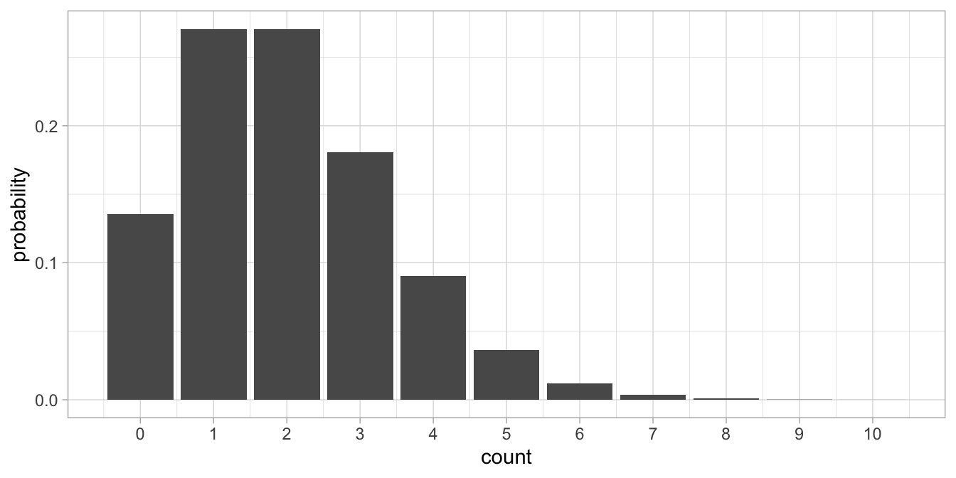
Figure 16.2: The Poisson probability distribution with lambda = 2.
What we see is that the values tend to cluster around the lambda parameter value of 2 (therefore we call \(\lambda\) a tendency parameter). We see only discrete values, and no values below 0. The distribution is not symmetrical, and we see a few extreme values such as those higher than 6. If we would take the mean of the distribution, we would find a value of 2. If we would compute the variance of the distribution we would also find 2. In general, if we have a Poisson distribution with a tendency parameter \(\lambda\), we know from theory that both the mean and the variance will be equal to \(\lambda\).
A Poisson model could be suitable for our data: a linear equation could predict the parameter \(\lambda\) and then the actual data show a Poisson distribution.
\[\begin{aligned} \lambda &= b_0 + b_1 X \\ Y &\sim Poisson(\lambda)\end{aligned}\]
However, because of the additivity assumption, the equation \(b_0 + b_1 X = \lambda\) can lead to negative values for \(\lambda\) if either \(b_0\) or \(b_1\) is negative, and/or if \(X\) has negative values. A negative value for \(\lambda\) is not logical, because we then would have a tendency to observe values like -2 and -4 in our data, which is contrary to having count data. A Poisson distribution always shows integers of at least 0, so one way or another we have to make sure that we always have a \(\lambda\) of at least 0.
Remember that we saw the reverse problem with logistic regression: there we wanted to have the possibility of negative values for our dependent variable logodds ratio, so therefore we used the logarithm. Here we want to always have positive values for our dependent variable, so we can use the inverse of the logarithm function: the exponential. Then we have the following model:
\[\begin{aligned} \lambda &= \textrm{exp}(b_0 + b_1 X)= e^{b_0+b_1X} \\ Y &\sim Poisson(\lambda)\end{aligned}\]
This is a generalised linear model, now with a Poisson distribution and an exponential link function. The exponential function makes any value positive, for instance \(\textrm{exp}(0)=1\) and \(\textrm{exp}(-10)=0.00005\), so that we always have a positive \(\lambda\) parameter.
Let’s analyse the film revenues data with this generalised linear model. Our dependent variable is Number of cinemas, that is, the number of cinemas that are running a particular film, and the independent variable is Rank, which indicates the relative amount of weekend gross revenu for that film (rank 1 meaning the most money). When we run the analysis, the result is as follows:
\[\begin{aligned} \lambda &= \textrm{exp}(6.450 -0.075 \times \texttt{Rank}) \\ \texttt{N}_{cinemas} &\sim Poisson(\lambda)\end{aligned}\]
What does it mean? Well, similar to logistic regression, we can understand such equations by making some predictions for interesting values of the independent variable. For instance, a value of 1 for Rank means that we are looking at the film with the largest gross revenu. If we fill in that value, we get the equation \(\lambda=\textrm{exp}(6.450 -0.075 \times 1)= \textrm{exp} (6.375)= 587\). Thus, for the top film of the week, we expect to see that the film runs in 587 cinemas.
Another value of Rank might be 10, representing the film with the 10th largest gross revenue. If we fill in that value, we get: \(\lambda=\textrm{exp}(6.450 -0.075 \times 10)= \textrm{exp}(5.70) = 299\). Thus, for the film with the 10th largest revenue, we expect to see that it runs in 299 cinemas.
If we look at the pattern in these expected scores, we see that the number of cinemas is negatively related to the gross revenue. That is what we find in this data set. In the next section we will see how to perform the analysis in R.
16.2 Poisson regression in R
Poisson regression is a form of a generalised linear model analysis,
similar to logistic regression, so we can use the glm() function to analyse the cinema data. Instead of using a Bernoulli
distribution, we use a Poisson distribution. The code is as follows.
model <- bfi %>%
  glm(`Number of cinemas` ~ Rank, family = poisson, data = .)
model %>% tidy(conf.int = T)
## # A tibble: 2 × 7
## term estimate std.error statistic p.value conf.low conf.high
## <chr> <dbl> <dbl> <dbl> <dbl> <dbl> <dbl>
## 1 (Intercept) 6.45 0.0173 372. 0 6.41 6.48
## 2 Rank -0.0747 0.00114 -65.7 0 -0.0769 -0.0725We see the same values for the intercept and the effect of Rank as in the previous section. We now also see 95% confidence intervals for these parameter values.
For interpretation and checking model assumptions, it is a good idea to make a visualisation of the model. We can let R plot the predicted counts next to the observed data using the following code:
bfi %>%
  add_predictions(model, type = "response") %>%
  ggplot(aes(x = Rank, y = `Number of cinemas`)) +
  geom_point() +
geom_line(aes(y = pred)) 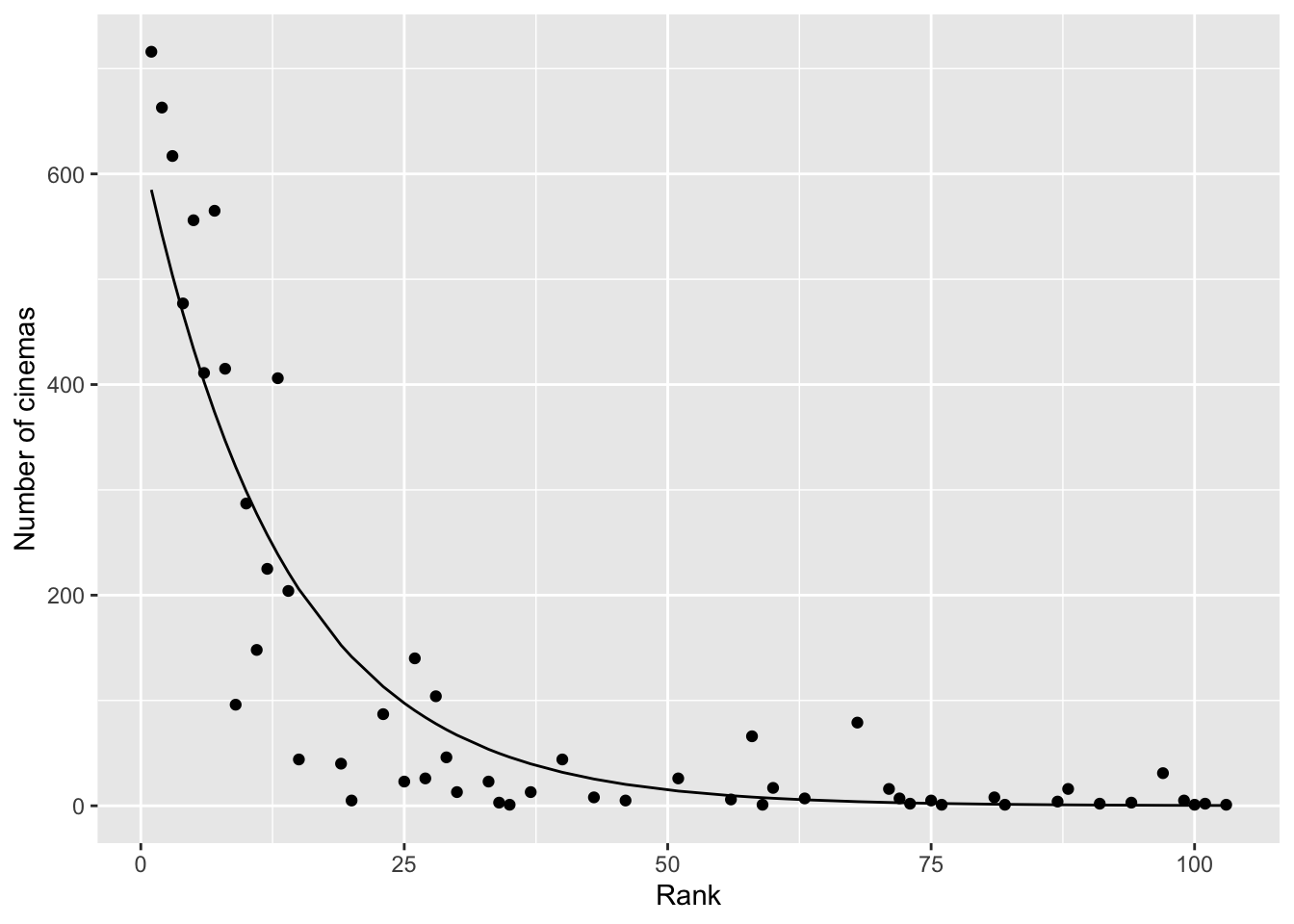
Note that the line with the predicted counts is curvy. The model equation \(b_0 + b_1 \textrm{Rank}\) is linear, that’s why we call the Poisson model a linear model, but through the exponential link function, \(\lambda = \textrm{exp}(b_0 + b_1 \textrm{Rank})\), we get a line that is not straight anymore.
Do we think the model is a good description of the data? It seems overall rather OK. We only see that for the highest ranked films (the first six films or so), the predicted numbers are generally too high (on the line or above it), and for the films that come next (ranks 7 to 25 or so), the predicted numbers are generally too low (all under the line). With a perfect model, the dots would all be on the line, or randomly distributed around. Some deviation from randomness is observed here.
Going back to the regression table, we see that for Rank, the confidence interval runs from -0.077 to -0.073. The value 0 is clearly not included in the confidence interval. We also see a test statistic for Rank, which is a \(z\)-statistic similar to that seen in logistic regression. Remember that the \(z\)-statistic is computed by \(b/SE\). For large enough samples, the \(z\)-statistic follows a standard normal distribution. From that distribution we know that a \(z\)-value of -65.7 is significant at the 5% level. The output tells us it has an associated \(p\)-value of less than 0.001.
However, what should we do with this information? Remember that the statistical test for a null-hypothesis only works if you have a random sample from population data. The first question that we should ask ourselves is whether we have a random sample of data here. The second question is, if we have a random sample of data, from what population was it randomly sampled?
We already get stuck at the first question, since clearly we did not obtain a random sample of data. All our data came from the last weekend of November 2023. The data can clearly be used to say something about that weekend, as most of the films were included in the data, but can they be used to say something about other weekends? Possibly not. Other weekends see different numbers of visitors and different kinds of visitors. It makes a difference if we are looking at a dark and gloomy weekend in November, a sunny weekend in July, or a weekend during the Christmas holidays when whole families go to the cinema. Some weekends on end there may be a huge blockbuster, that might also significantly alter the pattern in the data. It is therefore safest, when reporting this analysis, to stick to a description of the data set itself, and not generalise.
We can write:
"UK cinema data from 24-26 November 2023 were modelled using a generalised linear model with a Poisson distribution (Poisson regression), with independent variable rank and dependent variable the number of cinemas. The numbers of cinemas could reasonably be described by the equation \(\lambda = \textrm{exp}(6.45 - 0.075 \times \texttt{rank})\), where the films were ranked in terms of gross weekend revenu."
16.3 Overdispersion (advanced)
As we saw, with the Poisson distribution there is only one parameter, \(\lambda\). That means that if we model data with a Poisson distribution, the variance of the residuals should be exactly the same as the expected number.
Let’s look at the cinema data. We saw that a higher rank number was associated with a lower expected number of cinemas. Since a lower expected number should go together with a lower variance, according to the Poisson model, we should see that also in the data, otherwise the model is wrong. But also, the variance in numbers should be more or less equal to the average number. Let’s look at the distribution of the data, by first binning the data. We put the 8-top ranking films in the first bin (group), the next 8 films in the second bin, etcetera. Then for every bin we plot the distribution.
bfi %>%
  mutate(bin = cut_number(Rank, n = 8, boundary = 1)) %>%
  ggplot(aes(x = bin, y = `Number of cinemas`)) +
  geom_jitter(width = .1, height = 0, alpha = 0.5)  +
  geom_boxplot(aes(x = bin), alpha = .3) +
xlab("Bin for Rank") 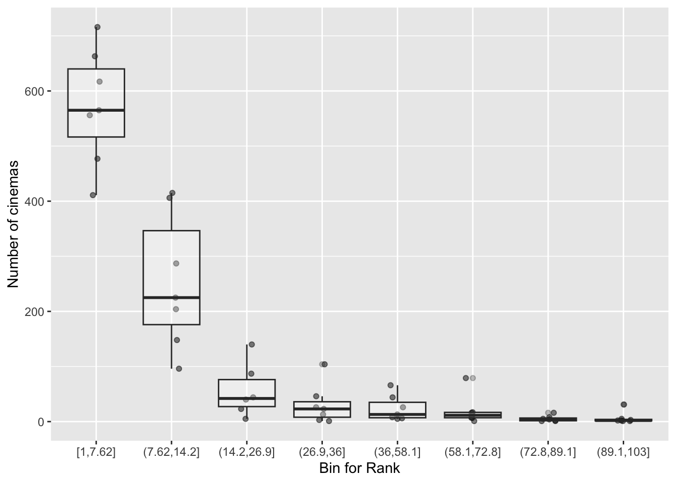
We see that the variance is larger when the values are larger, and becomes smaller when numbers become smaller. However, do the variances actually resemble the expected numbers? For every bin of 8 films, we compute the mean and the variance.
bfi %>%
  mutate(bin = cut_number(Rank, n = 8, boundary = 1)) %>%
  group_by(bin) %>%
  summarise(var = var(`Number of cinemas`),
            mean = mean(`Number of cinemas`)) %>%
  dplyr::select(bin, mean, var)
## # A tibble: 8 × 3
## bin mean var
## <fct> <dbl> <dbl>
## 1 [1,7.62] 572. 11049.
## 2 (7.62,14.2] 254. 14942.
## 3 (14.2,26.9] 56.5 2421.
## 4 (26.9,36] 30.9 1275.
## 5 (36,58.1] 24 538.
## 6 (58.1,72.8] 21.2 839.
## 7 (72.8,89.1] 5.29 28.6
## 8 (89.1,103] 6.43 119.For most of the bins, we see an average number that is lower than the corresponding variance. Clearly the variance does not match the mean. In statistics this is called overdispersion. There is a test to detect overdispersion in your data, available in the performance package.
## # Overdispersion test
##
##        dispersion ratio =  108.223
##   Pearson's Chi-Squared = 5627.584
##                 p-value =  < 0.001
Extensive treatment of dispersion is outside the scope of this book. The interested reader is referred to more specialised resources on generalised linear models.
But one option to deal with violations of the Poisson model assumptions that we will mention here is to try out alternative models. A well-known alternative to the Poisson model is the negative binomial model. The negative binomial model is similar to the Poisson model but more flexible (the Poisson distribution is a special case of the more general negative binomial distribution). It can be estimated with the glm.nb() function from the MASS package.
library(MASS)
model2 <- bfi %>%
  glm.nb(`Number of cinemas` ~ Rank, data = .)
check_overdispersion(model2)
## # Overdispersion test
##
## dispersion ratio = 0.582
## p-value = 0.64The negative-binomial model solves most of the overdispersion problem as the dispersion ratio drops dramatically. Below we see the expected counts for this model. Comparing this figure with that for the Poisson model, we see that it makes different predictions, especially for the top-ranked films. The predictions seem actually much worse for the top-ranked films, as the model underestimates the number of cinemas for the top 8 films.
bfi %>% add_predictions(model2, type = "response") %>%
  ggplot(aes(x = Rank, y = `Number of cinemas`)) +
  geom_point() +
geom_line(aes(y = pred)) 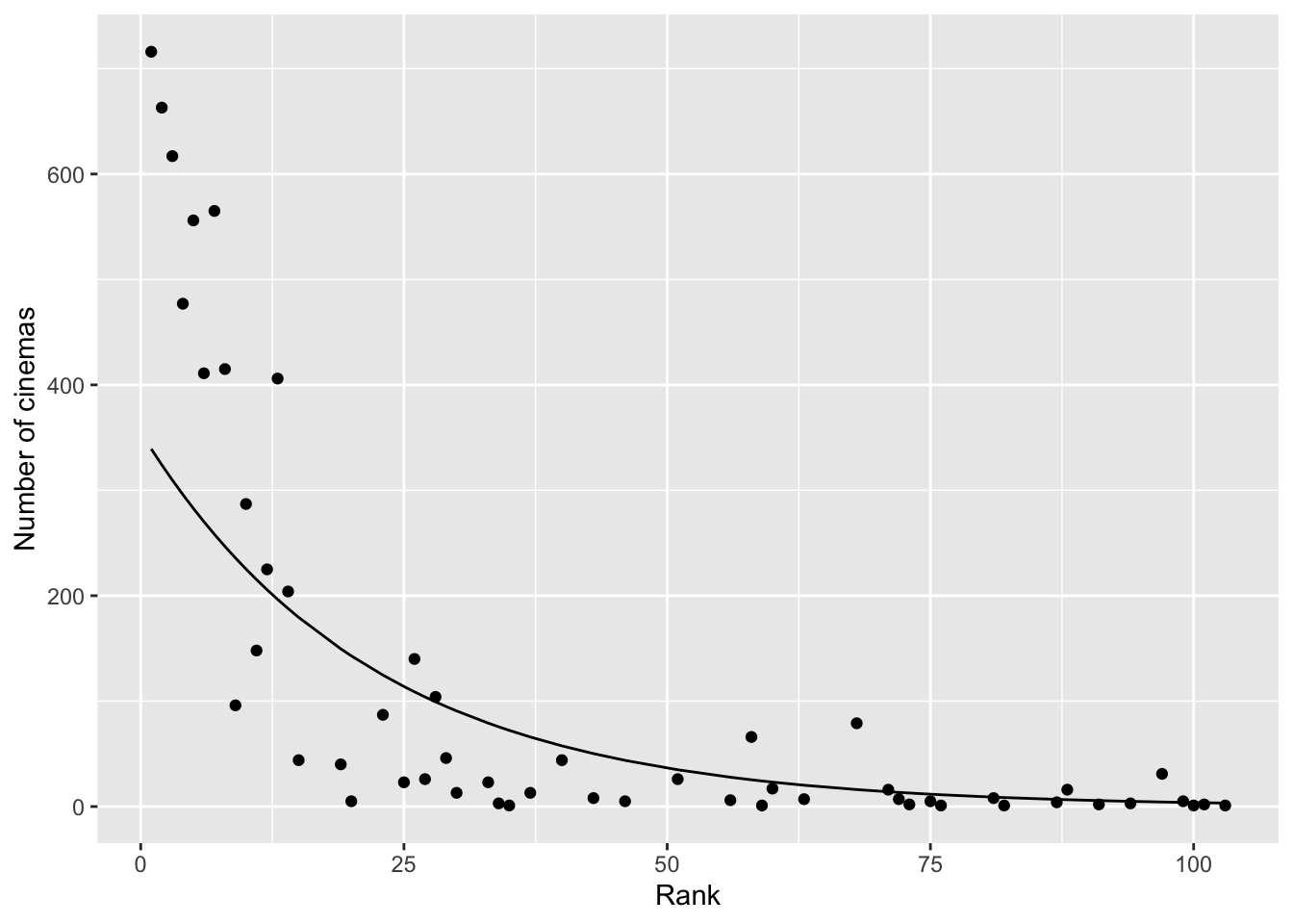
This problem is not easily solved. Instead of the ranks, we could work with the original data: the actual gross weekend revenue. Because this variable is extremely skewed (a few very large outliers), it makes sense to work with the logarithm of that variable and use that in the negative binomial model.
model3 <- bfi %>%
  glm.nb(`Number of cinemas` ~ log(`Weekend Gross`),
         data = .)

bfi %>%
  add_predictions(model3, type = "response") %>%
  ggplot(aes(x = log(`Weekend Gross`),
             y = `Number of cinemas`)) +
  geom_point() +
geom_line(aes(y = pred)) 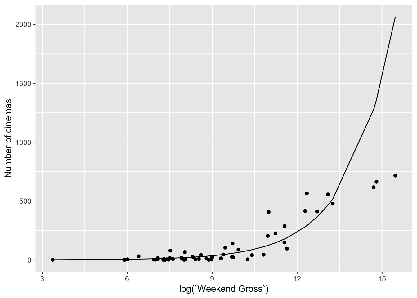
The negative binomial model shows a good fit for most of the data. The model is sadly not able to predict the three top films correctly. This model seems better than the model that used the ranks, since there the top 8 films were badly predicted.
16.4 Association between two categorical variables
Poisson models are used when you count things, and when you are interested in how two or more variables are associated. Let’s go back to Chapter 1. There we discussed the situation where we have two categorical variables, and you want to see how they co-vary. We made a crosstable that showed the counts of each combination of the levels of the categorical variables.
Imagine we do a study into the gender balance in companies. In one particularly large, imaginary company, there are about 100,000 employees. For a random sample of 1000 employees, we know their gender (female or male), and we know whether they have a position in senior management or not (leadership: yes or no). It turns out that there are 22 female senior managers, and only 8 male senior managers. If we would randomly pick a senior manager from this sample, they would more likely be a woman than a man, right? Can we therefore conclude that there is a positive gender bias, in that senior managers in this company are more often female? Think about it carefully, before you read on.
The problem is, you should first know how many men and how many women there are in the first place. Are there relatively many female leaders, given the gender distribution in this company? In Table 16.2 you find the crosstable of the data. From this table we see that there are 800 women in the sample and 200 men.
| gender | no | yes | Total |
|---|---|---|---|
| female | 778 | 22 | 800 |
| male | 192 | 8 | 200 |
| Total | 970 | 30 | 1000 |
Thus, we see see more female leaders than male leaders, but we also see many more women than men working there in the first place.
It is clear that the data in the table are count data. They can therefore be analysed using Poisson regression. Later in this chapter we will see how we can do that. But first we have to realise that the counts are a bit different from the counts we observed in the cinema example where we counted the number of cinemas than a particular film. The dependent variable there was a count variable, but it also had a clear meaning: the count reflected the choice of cinema directors to show a film.
In the example here, we simply count the number of employees in a data set that fit a set of criteria (i.e. being a woman and being a senior manager). Technically, both variables are count variables, but conceptually they might feel different for you.
Therefore, before we dive deeper into Poisson models, we will look at a very traditional way of analysing count data in crosstables: computing the Pearson chi-square statistic.
16.5 Cross-tabulation and the Pearson chi-square statistic
Table 16.2 shows that there were 800 women and 200 men in the data set, and of these there were in total 30 employees in senior management. Now if 30 people out of 1000 are in senior management, it means that a proportion of \(\frac{30}{1000}= 0.03\) are in senior management. You might argue that there is only a gender balance if that same proportion is observed in both men and women.
Let’s look at the proportion of women in senior management. We observe 22 female leaders out of a total of 800 women. That’s equal to a proportion of \(\frac{22}{800} = 0.0275\). That is quite close but not equal to 0.03.
Now let’s look at the men. We observe 8 male leaders out of a total of 200 men. That’s equal to a proportion of \(\frac{8}{200} = 0.04\). That is quite close but not equal to 0.03.
Relatively speaking, therefore, there are more men in a senior management role (4%) than there are women in a senior management role (2.75%). Overall there are more women leaders in this data set, but taking into account the gender ratio, there are relatively fewer women than men in the leadership.
Now the question remains whether this difference in leadership across gender is real. These data come from only one particular month, from only 1000 employees instead of all 100,000. Every month new people get hired, get fired, or simply leave. With a huge turn-over, the numbers change all the time. The question is whether we can generalise from these data to the whole company: is there a general gender bias in this company, or are the results we look at due to the random sampling?
The Pearson chi-square test is based on comparing that what you expect given a hypothesis, with what you actually observed. Suppose our hypothesis is that there is a perfect gender balance: the proportion of leaders among the women is equal to the proportion of leaders among the men.
Before we continue, we assume that the total numbers of both genders and the leadership positions are reflective of the actual situation. We therefore assume the proportion of women is 0.8 and the proportion of men is 0.2. We also assume the proportion of senior managers is 3% and the proportion of other employees is 97%.
Assuming gender balance, we expect that a proportion of 0.03 of the women are in a leadership position, and we also expect a proportion of 0.03 of the men are in a leadership position. Given there are 800 women in the data set, under the gender balance assumption we expect \(0.03\times 800 = 24\) women with a leadership role. Given there are 200 men, under the gender balance assumption we expect \(0.03 \times 200 = 6\) men with a leadership role.
Now that we have the number of people that we expect based on gender balance, we can compare them with the actual observed numbers. Let’s calculate the deviations of what we observed from what we expect.
We observed 22 women in a leadership position, where we expected 24, so that is a deviation of \(22-24=-2\) (observed minus expected).
We observed 8 men in the leadership, where we expected 6, which results in a deviation of \(8-6=+2\) (observed minus expected).
We also have the observed counts of the employees not in the leadership. Also for them we can calculate expected numbers based on gender balance. A proportion of .97 are not in the leadership. We therefore expect \(0.97 \times 800= 776\) women. We observed 778, so then we have a deviation of \(778-776 = +2\).
For the men we expect \(0.97\times 200 = 194\) to be without a leadership role, which results in a deviation of \(192 - 194 = -2\).
If we would add these deviations up, we should be able to say something about how much the observed numbers deviate from the expected numbers. However, if we do that, we get a total of 0, since half of the deviations are positive and half of them are negative. In order to avoid that and get something that is very large when the deviations are very different from 0, we could instead take the squares of these differences and then add them up (the idea is similar to that of computing the variance as an indicator of how much values deviate from each other). Another reason for taking the squares is that the sign of the deviation doesn’t really matter; it is only the distance from 0 that is relevant.
If we take the deviations, square them, and add them up, we get:
\[(-2)^2 + 2^2 + 2^2 + (-2)^2 = 16\] However, we should not forget that a deviation of 2 is only a relatively small deviation when the expected number is large, like 776. Observing 778 instead of the expected 776 is not such a big deal: it’s only a 0.26% increase. In contrast, if you expect only 6 people and suddenly you observe 8 people, that is relatively speaking a large difference (a 33% increase). We should therefore off-set the observed deviations from what we expected. We then get:
\[\frac{(-2)^2}{24} + \frac{2^2}{6} + \frac{2^2}{776} + \frac{(-2)^2}{194} = 0.86\]
What we actually did here was computing a test statistic that helps us to decide whether we have evidence in this data set that speaks against gender balance. It is called the Pearson chi-square statistic and it indicates to what extent the proportions observed in one categorical variable (say leadership membership vs non-membership) are different for the different categories of another categorical variable (say males and females). We observed different leadership proportions for males and females and this test statistic helps us decide if the proportions were also significantly different.
In formula form, the Pearson chi-square statistic looks like this:
\[X^2 = \sum_i \frac{(O_i-E_i)^2}{E_i}\]
For every cell \(i\) in the crosstable, here 4 cells, we compute the difference between the observed count (O) and expected count (E). We square these difference first, then divide them by the expected count, and the resulting numbers we add up (summation). As we saw, we ended up with \(X^2 = 0.86\).
If the null-hypothesis is true, the sampling distribution of \(X^2\) is a chi-square distribution. The shape of this distribution depends on the degrees of freedom, similar to the \(t\)-distribution. The degrees of freedom for Pearson’s chi-square are determined by the number of categories for variable 1, \(K_1\), and the number of categories for variable 2, \(K_2\): \(\textrm{df} = (K_1 - 1)(K_2 - 1)\). Thus, with a \(2 \times 2\) crosstable there is only one degree of freedom: \((2-1)\times(2-1)= 1\).
The chi-square distribution with one degree of freedom is plotted in Figure 16.3.
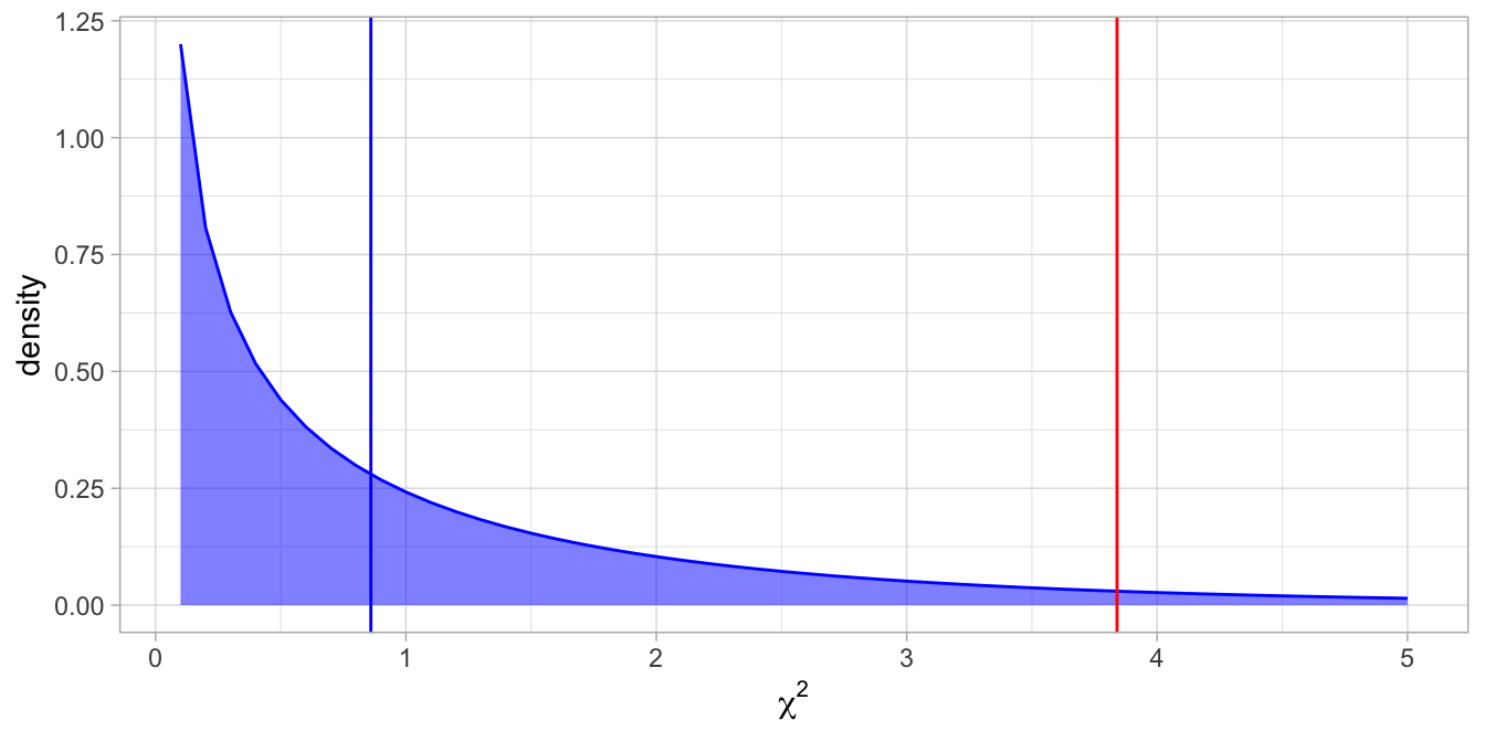
Figure 16.3: The chi-square distribution with one degree of freedom. Under the null-hypothesis we observe values larger than 3.84 only 5% of the time, indicated by the red line. The blue line represents the value based on the data.
The observed value of the test statistic is 0.86 and plotted in blue. The critical value for the null-hypothesis to be rejected at an alpha of 5% is 3.84 and depicted in red. The null-hypothesis can clearly not be rejected. There is no evidence that there is any gender imbalance in this large company of 100,000 employees.
16.6 Pearson chi-square in R
The Pearson chi-square test is based on data from a crosstable. The data that you have are most often not in such a format, so you have to create that table first.
Suppose you have the dataframe with the 1000 employees. We have the variable ID of the employee, a variable for the gender, and a variable for whether they are in senior management.
The top rows of the data might look like this:
## # A tibble: 3 × 3
##      ID gender leader
##   <int> <chr>  <chr>
## 1     1 male   no
## 2     2 male   no
## 3     3 male   no
As we saw in Chapter 1, we can create a table with the tabyl() function from the janitor package.
##  gender  no yes
##  female 778  22
##    male 192   8
Next we plug the crosstable into the function chisq.test().
##
##  Pearson's Chi-squared test with Yates' continuity correction
##
## data:  companytable
## X-squared = 0.48325, df = 1, p-value = 0.487
Two things strike us: the value for the X-squared is not equal to the 0.86 that we computed by hand. But we also see that R used Yates’ continuity correction. This continuity correction is important if some of your expected cell counts are rather low. Here we saw that we expected only 6 men in senior management.
If we don’t let R apply this continuity correction, we obtain our manually computed statistic of 0.86:
##
##  Pearson's Chi-squared test
##
## data:  companytable
## X-squared = 0.85911, df = 1, p-value = 0.354
Generally you should use the corrected version. We then report:
"Using data on 1000 employees the observed proportion of women in a leadership role was 0.0275. The observed proportion of men in a leadership role was 0.04. A Pearson chi-square test with continuity correction showed that this difference was not significant, \(X2(1) = 0.48\), \(p = 0.487\). The null-hypothesis that the proportions are equal in the population could not be rejected."
16.7 Analysing crosstables with Poisson regression in R
If we want to analyse the same data with a Poisson regression, we need to create a dataframe with a count variable. We start from the original dataframe companydata and count the number of men and women with and without a senior management role.
## # A tibble: 3 × 3
##      ID gender leader
##   <int> <chr>  <chr>
## 1     1 male   no
## 2     2 male   no
## 3 3 male no## # A tibble: 4 × 3
## # Groups: gender [2]
## gender leader count
## <chr> <chr> <int>
## 1 female no 778
## 2 female yes 22
## 3 male no 192
## 4 male yes 8We now have a dataframe with the count data in long format, exactly what we need for the Poisson linear model. We take the count variable as dependent variable, and let gender and leader be the predictors:
##
## Call:  glm(formula = count ~ gender + leader, family = poisson, data = .)
##
## Coefficients:
## (Intercept)   gendermale    leaderyes
##       6.654       -1.386       -3.476
##
## Degrees of Freedom: 3 Total (i.e. Null);  1 Residual
## Null Deviance:       1503
## Residual Deviance: 0.8003    AIC: 31.27
In the output we see that the effect of being male is negative, saying that there are fewer men than women in the data. The leadership effect is also negative: there are fewer people in a leadership role than people not in that role.
We can look at what the model predicts regarding the counts:
## # A tibble: 4 × 4
## # Groups:   gender [2]
##   gender leader count  pred
##   <chr>  <chr>  <int> <dbl>
## 1 female no       778 776.
## 2 female yes       22  24.0
## 3 male   no       192 194.
## 4 male   yes        8   6
You see that the model makes the same predictions as under the assumption that there is a gender balance. The deviations in the observed compared to the predicted (expected) are 2 again, similar as we saw when computing the chi-square test. We want to know however, whether the ratio of leaders is the same in males and females: in other words whether the effect of leadership on counts is different for men and women. We therefore check if there is a significant gender by leader interaction effect.
model2 <- companycounts %>%
  glm(count ~ gender + leader + gender:leader,
      family = poisson, data = .)
model2 %>% tidy()
## # A tibble: 4 × 5
## term estimate std.error statistic p.value
## <chr> <dbl> <dbl> <dbl> <dbl>
## 1 (Intercept) 6.66 0.0359 186. 0
## 2 gendermale -1.40 0.0806 -17.4 1.55e-67
## 3 leaderyes -3.57 0.216 -16.5 4.12e-61
## 4 gendermale:leaderyes 0.388 0.421 0.921 3.57e- 1We see a positive interaction effect: the specific combination of being a male and a leader, has an extra positive effect of 0.388 on the counts in the data. The effect is however not significant, since the \(p\)-value is .357.
We see that the \(p\)-value is very similar to the \(p\)-value for the uncorrected Pearson chi-square test (.354) and different from the corrected one (.487). Every \(p\)-value with these kinds of analyses is only an approximation. The \(p\)-values are dissimilar here because the expected number of males in a senior management role is pretty low. For data sets with higher counts, the differences between the methods will disappear. Generally, the Pearson chi-square with continuity correction gives you best results for relatively low expected counts (counts of 5 or less).
If you would like to report the results form this Poisson analysis instead of a Pearson chi-square test, you could write:
"Using data on 1000 employees the observed proportion of women in a leadership role was 0.0275. The observed proportion of men in a leadership role was 0.04. A Poisson regression with number of employees as the dependent variables and main effects of gender, leadership and their interaction showed a non-signficant interaction effect, \(B = 0.388\), \(SE = 0.421\), \(z = 0.92\), \(p = .357\). The null-hypothesis that the proportions are equal in the population could not be rejected."
If the data set is large enough and the numbers are not too close to 0, the same conclusions will be drawn, whether from a \(z\)-statistic for an interaction effect in a Poisson regression model, or from a cross-tabulation and computing a Pearson chi-square. The advantage of the Poisson regression approach is that you can do much more with them, for instance more than two predictors, and including also numeric variables as predictors. In the Poisson regression, you also make it more explicit that when computing the \(z\)-statistic, you take into account the main effects of the variables (the row and column totals). You do that also for the Pearson chi-square, but it is less obvious: we did that by first calculating the proportion of males and females and then calculating the overall proportion of senior management roles, before calculating the expected numbers. The next section shows that you can more easily answer advanced research questions with Poisson regression than with Pearson’s chi-squares and crosstables.
16.8 Going beyond 2 by 2 crosstables (advanced)
If your categorical variables have more than 2 categories you can still do a Pearson chi-square test. You only run into trouble when you have more than two categorical variables, and you want to study the relationship between them. Let’s turn to an example with three categorical variables. Suppose in the employee data, we have data on gender, leadership role, and also whether people work either at the head office in central London, or whether they work at one of the dozens of distribution centres across the world. Do we see a different gender bias in the head office compared to the distribution centres?
Let’s have a look at the data again. Now we make separate tables, one for the head office and one for the distribution centres, see Figure 16.4.
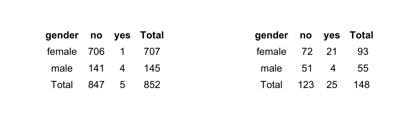
Figure 16.4: The crosstables of gender and leadership, separately for the distribution centres (left table) and the head office (right table).
Remember that in the complete data set, we observed 4% of leadership in the men and 2.75% in the women. Now let’s look only at the data from the distribution centres. Out of 707 women, 1 of them is in senior management, leading to a proportion of 0.001. Out of 145 men, 4 of them are a senior manager, leading to a proportion of 0.028. Thus, at the distribution centres there seems to be a gender bias in that men tend to be more often in senior management positions than women, taking into account overall differences in gender representation.
Contrast this with the situation at the head office in London. There, 21 out of 93 women are in senior management, a proportion of 0.23. For the men, 4 out of 55 are in senior management, a proportion of 0.07. Thus, at the head office, senior management positions are relatively speaking more prevalent among the women than the men. The opposite of what we observed in the distribution centres.
The next question is then, can we generalise this conclusion to the population of the entire company: is the gender bias different at the two types of location? For that we can do a Poisson analysis. First we prepare the data in such a way that for every combination of gender, leadership and location, we get a count. We do that in the following way.
## # A tibble: 3 × 4
##      ID gender leader location
##   <int> <chr>  <chr>  <chr>
## 1   182 female yes    distribution
## 2   197 female yes    headoffice
## 3   231 female yes    headoffice
companycounts <- companydata_location %>%
group_by(gender, leader, location) %>%
summarise(count = n()) %>%
arrange(location)
companycounts## # A tibble: 8 × 4
## # Groups: gender, leader [4]
## gender leader location count
## <chr> <chr> <chr> <int>
## 1 female no distribution 706
## 2 female yes distribution 1
## 3 male no distribution 141
## 4 male yes distribution 4
## 5 female no headoffice 72
## 6 female yes headoffice 21
## 7 male no headoffice 51
## 8 male yes headoffice 4Next, we apply a Poisson regression model. We predict the counts by taking the gender totals, the leader totals and the location totals.
##
## Call:  glm(formula = count ~ gender + leader + location, family = poisson,
##     data = .)
##
## Coefficients:
##        (Intercept)          gendermale           leaderyes  locationheadoffice
##              6.494              -1.386              -3.476              -1.750
##
## Degrees of Freedom: 7 Total (i.e. Null);  4 Residual
## Null Deviance:       2168
## Residual Deviance: 117.9     AIC: 166.4
Generally, there are fewer males, fewer leaders, and fewer people in the head office compared to the other categories. In the previous analysis we saw that a gender bias in leadership was modelled using an interaction effect. Now that we have data on location, there could in addition be a gender bias in location (relatively more women in the head office), and a location bias in leadership (relatively more leaders in the head office). We can therefore add these three two-way interaction effects. But most importantly, we want to know whether the gender bias in management (the interaction between gender and leadership) is moderated by location. This we can test by adding a three-way interaction effect: gender by leader by location. Putting it all together we get the following R code:
companycounts %>%
  glm(count ~ gender + leader + location +
        gender:leader + gender:location + leader:location +
        gender:leader:location,
      family = poisson, data = .)
The exact same model can be achieved with less typing, by using the * operator: then you get all main effects, two-way interaction effects and the three-way interaction effect automatically:
## # A tibble: 8 × 5
##   term                                    estimate std.error statistic  p.value
##   <chr>                                      <dbl>     <dbl>     <dbl>    <dbl>
## 1 (Intercept)                                 6.56    0.0376    174.   0
## 2 gendermale                                 -1.61    0.0922    -17.5  2.73e-68
## 3 leaderyes                                  -6.56    1.00       -6.56 5.56e-11
## 4 locationheadoffice                         -2.28    0.124     -18.5  4.90e-76
## 5 gendermale:leaderyes                        3.00    1.12        2.67 7.55e- 3
## 6 gendermale:locationheadoffice               1.27    0.205       6.18 6.53e-10
## 7 leaderyes:locationheadoffice                5.33    1.03        5.17 2.37e- 7
## 8 gendermale:leaderyes:locationheadoffice    -4.31    1.26       -3.42 6.29e- 4
The only parameter relevant for our research question is the last one concerning the gender by leader by location interaction effect. Its value -4.31 is negative, indicating that the particular combination of being male, being a leader and working at the head office leads to a relatively lower count. There is thus a gender by location bias in leadership, in that the males are relatively more present in leadership positions at the distribution centres than at the head office. The effect is significant, so we can conclude that the gender bias shows a different pattern at the head office than at the distribution centres.
We report:
"Using data on 1000 employees the observed proportion of women in a leadership role was 0.0275. The observed proportion of men in a leadership role was 0.04. Taking into account differences across location we saw that women at distribution centres were relatively less often in senior management position than men (0.1% vs. 2.8%). At the head office, women were relatively more often in a senior management position than men (23% vs. 7%). A Poisson regression with number of employees as the dependent variables and main effects of gender, leadership, location and all their two-way and three-way interaction effects showed a significant three-way interaction effect, \(B = -4.31\), \(SE = 1.26\), \(z = -3.42\), \(p < .001\). The null-hypothesis that the gender bias is equal in the two types of locations of the company can be rejected."
16.9 Take-away points
A Poisson regression model is a form of a generalised linear model.
Poisson regression is appropriate in situations where the dependent variable is a count variable (\(0, 1, 2, 3, \dots\)).
Whereas the normal distribution has two parameters (mean \(\mu\) and variance \(\sigma^2\)), the Poisson distribution has only one parameter: \(\lambda\).
A Poisson distribution with parameter \(\lambda\) has mean equal to \(\lambda\) and variance equal to \(\lambda\).
\(\lambda\) can take any real value between 0 and \(\infty\).
Poisson models can be used to analyse crosstable data. This can also be done using Pearson’s chi-square, but Poisson models allow you to easily go beyond two categorical variables, and include numerical predictors.