Chapter 15 Generalised linear models: logistic regression
15.1 Introduction
In previous chapters we were introduced to the linear model, with its basic form
\[\begin{aligned} Y &= b_0 + b_1 X_1 + \dots + b_n X_n + e \\ e &\sim N(0, \sigma_e^2)\end{aligned}\]
Two basic assumptions of this model are the additivity in the parameters, and the normally distributed residual \(e\). Additivity in the parameters means that the effects of intercept and the independent variables \(X_1, X_2, \dots X_n\) are additive: the assumption is that you can sum these effects to come to a predicted value for \(Y\). So that is also true when we include an interaction effect to account for a moderation,
\[\begin{aligned} Y &= b_0 + b_1 X_1 + b_2 X_2 + b_3 X_1 X_2 + e \\ e &\sim N(0, \sigma_e^2)\end{aligned}\]
or when we use a quadratic term to account for another type of non-linearity in the data:
\[\begin{aligned} Y &= b_0 + b_1 X_1 + b_2 X_1 X_1 + e \\ e &\sim N(0, \sigma_e^2)\end{aligned}\]
In all these models, the assumption is that the effects of the parameters (\(b_0\), \(b_1\), \(b_2\)) can be summed.
The other major assumption of linear (mixed) models is the normal distribution of the residuals. As we have seen in for instance Chapter 7, sometimes the residuals are not normally distributed. Remember that with a normal distribution \(N(\mu,\sigma^2)\), in principle all values between \(-\infty\) and \(+\infty\) are possible, but they tend to concentrate around the mean \(\mu\), in the shape of the bell-curve.
A normal distribution is suitable for continuous dependent variables. Most measured variables are however not continuous at all. Think for example of temperature: if a thermometer gives degrees Celsius with a precision of 1 decimal, the actual data will in fact be discrete, showing rounded values like 10.1, 10.2, 10.3, but never any values in between.
Nevertheless, the normal distribution can still be used in many such cases. Take for instance a data set where the temperature in Amsterdam in summer was predicted on the basis of a linear model. Fig 15.1 shows the distribution of the residuals for that model. The temperature measures were discrete with a precision of one tenth of a degree Celsius, but the distribution of the residuals seems well approximated by a normal curve.
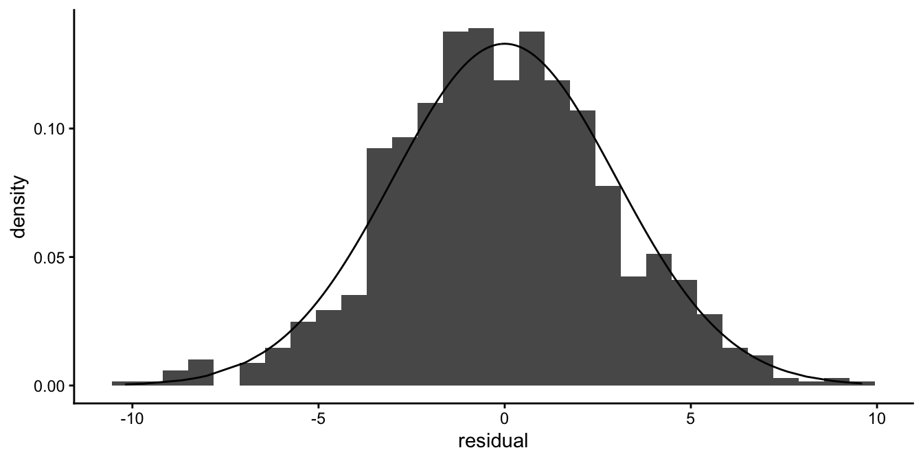
Figure 15.1: A histogram of residuals with a normal curve (black line). Even if measures are in fact discrete, the normal distribution can be a good approximation of the distribution of the residuals.
But let’s look at an example where the discreteness is more prominent. In Figure 15.2 we see the residuals of an analysis of test results. Students had to do an assignment that had to meet four criteria: 1) originality, 2) language, 3) structure, and 4) literature review. Each criterion was registered as either fulfilled (1) or not fulfilled (0). The total score for the assignment was determined on the basis of the number of criteria that were met, so the scores could be 0, 1, 2, 3 or 4. We call such a variable a count variable. In an analysis, this score was predicted on the basis of the average test score on previous assignments, using a linear model.
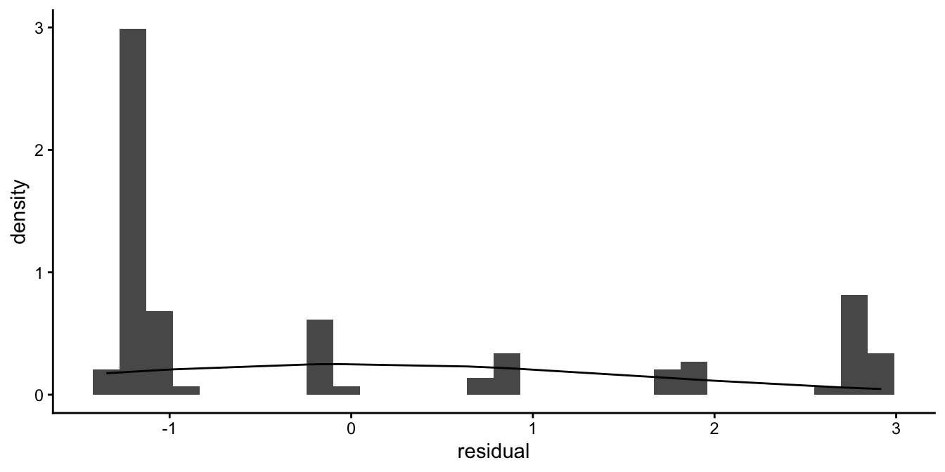
Figure 15.2: Count data example where the best fitting normal distribution is not a good approximation of the distribution of the residuals.
Figure 15.2 shows that the residuals are very discrete, and that a normal distribution with the same mean and variance is a very bad approximation of the distribution. We often see this phenomenon when our dependent variable has only a limited number of possible values.
An even more extreme case we observe when our dependent variable consists of only two values. For example, suppose our dependent variable is whether or not students passed the assignment: only those assignments that fulfilled all four criteria are regarded as sufficient. If we score all students who passed as 1 and score all students who failed as 0 and we predict this 0/1 score by the average test score on previous assignments using a linear model, we get the residuals displayed in Figure 15.3.
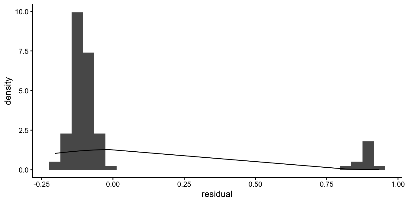
Figure 15.3: Dichotomous data example where the best fitting normal distribution is not a good approximation of the distribution of the residuals.
Here it is also evident that a normal approximation of the residuals will not do. When the dependent variable has only two possible values, a linear model will never work because the residuals can never have a distribution that is even remotely looking normal.
In this chapter and the next we will discuss how generalised linear models can be used to analyse data sets where the assumption of normally distributed residuals is not tenable. First we discuss the case where the dependent variable has only two possible values (dichotomous dependent variables like yes/no or pass/fail, heads/tails, 1/0). In Chapter 16, we will discuss the case where the dependent variable consists of counts (\(0, 1, 2, 3, 4, 5, \dots\)).
15.2 Example data with dichotomous outcome
Imagine that we analyse results on a simple reading test for children in first grade. These children are usually either 6 or 7 years old, depending on what month they were born in. The test is every year around February 1st. A researcher wants to know whether the age of the child can explain why some children pass the test and others fail. She collects data in a random sample of first grade pupils. She computes the age of the child in months. Each child that passes the test gets a score of 1 and all the others get a score of 0. Figure 15.4 plots the data.
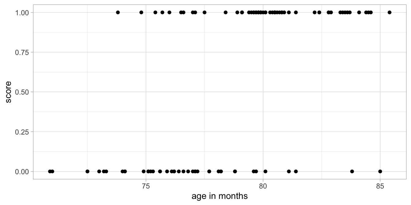
Figure 15.4: Data example: Test outcome (score) as a function of age, where 1 means pass and 0 means fail.
She wants to use the following linear model:
\[\begin{aligned} \texttt{score} &= b_0 + b_1 \texttt{age} + e \\ e &\sim N(0, \sigma_e^2)\end{aligned}\]
Figure 15.5 shows the data with the estimated regression line and Figure 15.6 shows the distribution of the residuals as a function of age.
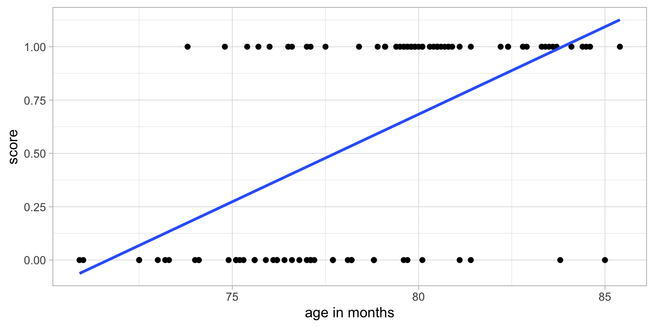
Figure 15.5: Example test data with a linear regression line.
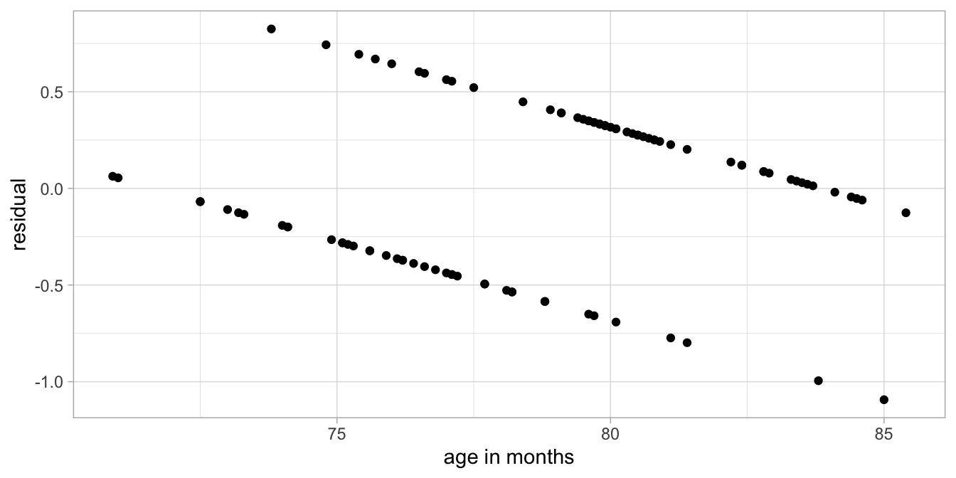
Figure 15.6: Residuals as a function of age, after a linear regression analysis of the test data.
Clearly, a linear model is not appropriate. The assumption of the linear model is that the residuals are scattered randomly around 0. This is not the case here as we see a clear pattern in the residuals. The main problem is that the dependent variable score has only two possible values: 0 and 1. When we have a dependent variable that is dichotomous or binary (only two values), we generally use logistic regression. The basic idea is that instead of assuming the normal distribution for the residuals, we assume the Bernoulli distribution.
15.3 Alternative: the Bernoulli distribution
Before we introduce the Bernoulli distribution, we go back to the regular linear model and rewrite it a bit. First we write the linear equation that gives us the expected value of the dependent variable, \(\hat{Y}\).
\[\begin{equation} \hat{Y} = b_0 + b_1 X_1 + b_2 X_2 \end{equation}\]
Next, we state that the actual observed value, \(Y\), depends on the expected or predicted value \(\hat{Y}\), and is normally distributed around that expected value, with a a certain variance \(\sigma^2\):
\[\begin{equation} Y \sim N(\hat{Y}, \sigma^2) \end{equation}\]
In this case, we omit the residual \(e\), but of course it is still there in the form of the difference between the observed value \(Y\) and the expected value \(\hat{Y}\), and this difference will have a normal distribution. The important thing to note here is that we split the linear model into two parts: a linear part, consisting of the linear equation to model \(\hat{Y}\), and the distribution part, consisting of a normal distribution for the observed value \(Y\).
This division into linear equation and distribution is the basic idea of generalised linear models. These models are all linear in that they all have the same type of linear equation part, but they differ in what kind of distribution they use. Here we model \(Y\) has having a normal distribution. Instead, we could use a distribution that is more suitable for a \(Y\) variable that only has two outcomes: the Bernoulli distribution.
A typical example where the Bernoulli distribution is appropriate is the flip of a coin. For a coin flip there are only two possible outcomes: heads or tails. For a fair coin, the probability of heads is 50%. That means that if we flip the coin 100 times, we expect to see heads in 50% of the cases. If the coin is not fair, for example when the probability of heads is 0.4, we can expect that if we flip the coin 100 times, on average we expect to see 40 times heads and 60 times tails. Our best bet then is that the outcome is tails. However, if we actually flip the coin, we might see heads anyway. Even though tails is more likely than heads, we never know when we will observe heads and when we will observe tails. There is some randomness. This is the kind of randomness that is modelled with the Bernoulli distribution. Let \(Y\) be the outcome of a coin flip: heads or tails. We model a Bernoulli distribution for variable \(Y\) with probability \(p\) for heads, in the following way:
\[Y \sim Bern(p_{heads})\] If we regard \(Y\) to be the outcome of a coin flip, the \(p_{heads}\) parameter tells us how often on average we can see heads rather than tails.
The same kind of randomness and unpredictability is true for the normal distribution in the linear model case: we expect that the observed value of \(Y\) is exactly equal to its predicted value, \(\hat{Y}\), but we observe a value for \(Y\) that is usually different from \(\hat{Y}\). This difference between predicted and observed is the residual. For a whole group of observations with the same predicted value for \(Y\), we know that the whole group of data points will show normal distribution around this predicted value, but we’re completely unsure what the residual will be for each individual data point.
\[Y \sim N(\hat{Y}, \sigma^2_e)\]
In our example of passing the test by the first graders, passing the test or not could also be conceived as the outcome of a coin flip: pass instead of heads and fail instead of tails. So would it be an idea to predict the probability of passing the test on the basis of age? And then for every predicted probability, we allow for the fact that actually the observed success for each individual child can differ. Our linear model could then look like this:
\[\begin{eqnarray} p_i &= b_0 + b_1 \texttt{age}_i \tag{15.1}\\ \texttt{score}_i &\sim Bern(p_i) \tag{15.2} \end{eqnarray}\]
So for each child \(i\), we predict the probability of passing the test, \(p_i\), on the basis of their age. Next, the randomness in the data comes from the fact that a probability is only a probability, so that the observed passing or failing of a child \(\texttt{score}_i\), is like a coin toss with probability of \(p_i\) for success. This can account for the observation that children with the exact same age, can still score differently on the test.
If we would apply such a model to the data, we end up with the following equation:
\[p = -5.876 + 0.082 \times \texttt{age}\]
This equation means that for a child with an age of 80 months, we have a probability of passing the test equal to \(-5.876 + 0.082 \times 80 = 0.68\). Now let’s look at the prediction for a child aged 71 months (a month before their sixth birthday). We then end up with \(-5.876 + 0.082 \times 71 = -0.05\). This can’t however be a probability: a probability is defined to be a number between 0 and 1. A similar problem we get when we do the calculations for a child aged 84 months (shortly after their seventh birthday): \(-5.876 + 0.082 \times 84 = 1.02\). Again, a value that can’t be a probability.
Therefore, in general, a linear equation that yields probabilities directly does not work. With a linear equation we can always end up with values less than 0 and more than 1, which can’t be probabilities. That means that in addition to a Bernoulli distribution, we need a trick that ensures we always get a probability between 0 and 1. The trick that is used is using log-odds.
15.4 Log-odds
To solve the problem with probabilities is that instead of using probabilities in the linear equation, we use log-odds. Log-odds are defined as the natural logarithm of the odds. First we briefly explain what odds are, and next we briefly explain what the logarithm is.
15.4.1 Odds
When talking about probabilities, one often also talks about odds, most often in the context of sports and gambling. In the context of our example data, the odds of passing the test is the ratio of the probability passing a test, and the probability of not passing the test.
\[\begin{equation} \texttt{odds}_{pass} = \frac{p_{pass}}{p_{fail}} \end{equation}\]
In general, we calculate the odds by dividing the probability \(p\) by its complement:
\[\begin{equation} \texttt{odds} = \frac{p}{1-p} \end{equation}\]
More on odds
Odds are an alternative way of expressing the likelihood of a particular event. They are used a lot in betting and gambling settings. Take for example the rolling of a dice. The probability of rolling a 6 is equal to \(\frac{1}{6}\) because there are 6 different types of outcome, and only one of them is “rolling a 6”. We say the probability is “one out of six”. For probabilities therefore, we calculate the number of events that lead to success and we divide by the total number of events.
In contrast, with odds, we count the number of outcomes that lead to success and we divide that by the number of outcomes that lead to failure. There is one outcome for success (“6”), and five outcomes for failure (“1, 2, 3, 4, or 5”). The odds ratio is then “one to five”, which is usually written as 1:5, but is equal to \(\frac{1}{5}\).
Instead of counting events you can also use the probability directly to come up with odds. The probability of a six is \(\frac{1}{6}\) and the probability of not a six is \(\frac{5}{6}\). The odds can then be computed by taking the ratio of these two probabilities: \(\frac{1/6}{5/6}= \frac{1}{5}\). In general, the odds of an event is the probability of that event \(p\) divided by probability of that event not happening, \(q = 1-p\),
\[\begin{equation} \texttt{odds} = \frac{p}{1-p} \end{equation}\]
Suppose the probability of winning the lottery is \(1\%\). Then the probability of losing is \(99\%\). A probability of \(1\%\) means that if I play the lottery a total of 100 times, I expect to win 1 time and lose 99 times. That means once in a total of 100 times: \(\frac{1}{100}\). In contrast, the odds are the number of events that are successful divided by the number of events that are unsuccessful, therefore 1:99, or \(\frac{1}{99}\).
Now that we know how to go from probability statements to statements about odds, how do we go from odds to probability? If someone says the odds of heads against tails is 10 to 1, this means that for every 10 heads (success), there will be 1 tails (failure). In other words, if there were 11 coin tosses in total, 10 would be heads and 1 would be tails. We can therefore transform odds back to probabilities by noting that 10 out of 11 coin tosses is heads, so \(10/11 = 0.91\), and 1 out of 11 is tails, so \(1/11=0.09\).
As a last example, if at the horse races, the odds of Bruno winning
against Sacha are four to five (4:5), this means that for every 4
winnings by Bruno, there would be 5 winnings by Sacha. So out of a total
of 9 winnings, 4 will be by Bruno and 5 will be by Sacha. The
probability of Bruno outrunning Sacha is then \(\frac{4}{9}=0.44\).
When transforming odds into probabilities, you can use the following equation:
\[\begin{equation} \tag{15.3} p = \frac{\texttt{odds}}{\texttt{odds} + 1} \end{equation}\]
15.4.2 Natural logarithm
The logarithm is closely related to the concept of the exponent. The exponent tells us how many times to use a number in a multiplication. In \(4^2\) the exponent “2” says to use 4 twice in a multiplication, so \(4^2 = 4 \times 4 = 16\). Similarly, \(4^3\) means we have to use 4 three times: \(4^3 = 4 \times 4 \times 4 = 64\).
When using the logarithm we go in reverse: How many of one number do we have to use in a multiplication to make another number. For example, if we want to know how often we have to use 4 in a multiplication to obtain 16, this is the same as asking about the logarithm of 16 with base 4, \(\texttt{log}_4(16)\). We know that if we multiply \(4 \times 4\), we obtain 16. Therefore,
\[\begin{equation} \texttt{log}_4(16) = 2 \end{equation}\]
Instead of base 4, we can also use other numbers. For example, we can use base 2:
\[\begin{equation} \texttt{log}_2(16) = 4 \end{equation}\]
because if we multiply 2 four times, we obtain 16: \(2 \times 2 \times 2 \times 2 = 2^4 = 16\).
A special case is using the number \(e\) as the base of our logarithm. The value of \(e\) is called Euler’s number and is about 2.7. When using \(e\) as the base we often write \(\ln\) instead of \(\textrm{log}_e\). For example,
\[\begin{equation} \log_{e}(16) = \texttt{ln}(16) \approx 2.77 \end{equation}\]
because if we raise \(e\) to the power 2.77, we get 16: \(e^{2.77} \approx 16\). An alternative way of writing \(e^{2.77}\) is \(\exp{(2.77)}\).
When using \(e\) as the base of the logarithm, we call it the natural logarithm.
15.4.3 Transforming probability into log-odds
A probability \(p\) is always between 0 and 1. If we transform a probability \(p\) into odds, we always end up with a number somewhere between 0 and infinity. For example if we use a small probability like 0.1, the corresponding odds is \(\frac{0.1}{0.9} \approx 0.11\). If we use a large probability like 0.9, the corresponding odds is \(\frac{0.9}{0.1} \approx 9\).
If we next take the natural logarithm of the odds, we end up with values that can be both positive and negative, in fact all values between \(-\infty\) and \(+\infty\) are possible. For example, with a probability of 0.1, the odds are 0.11 and the natural logarithm of 0.11 equals \(\ln(0.11) = -2.2\). With a probability of 0.9, the odds are 9 and the natural logarithm of 9 equals \(\ln(9) = +2.2\). The natural logarithm of the odds is called the log-odds.
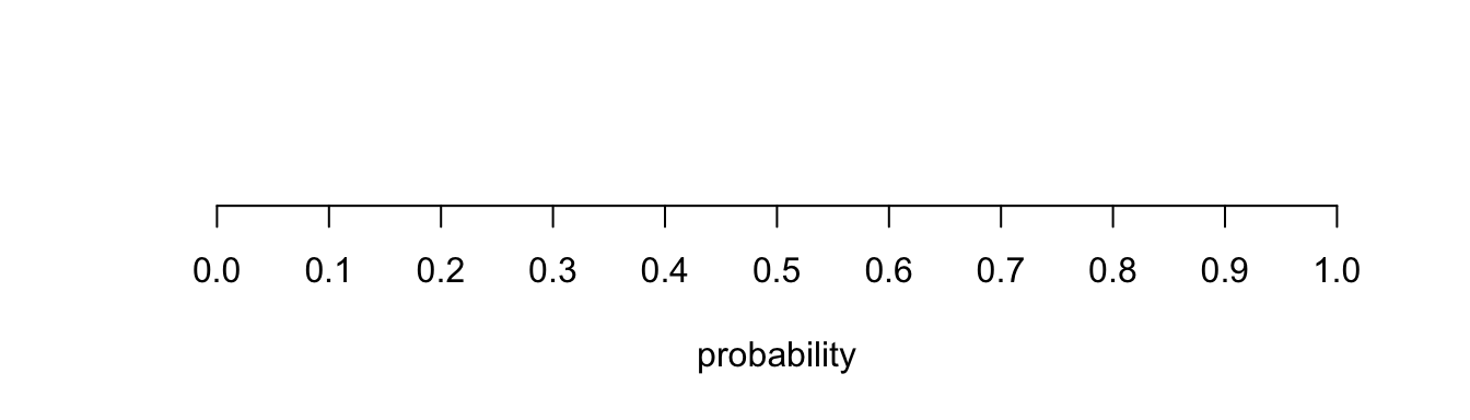
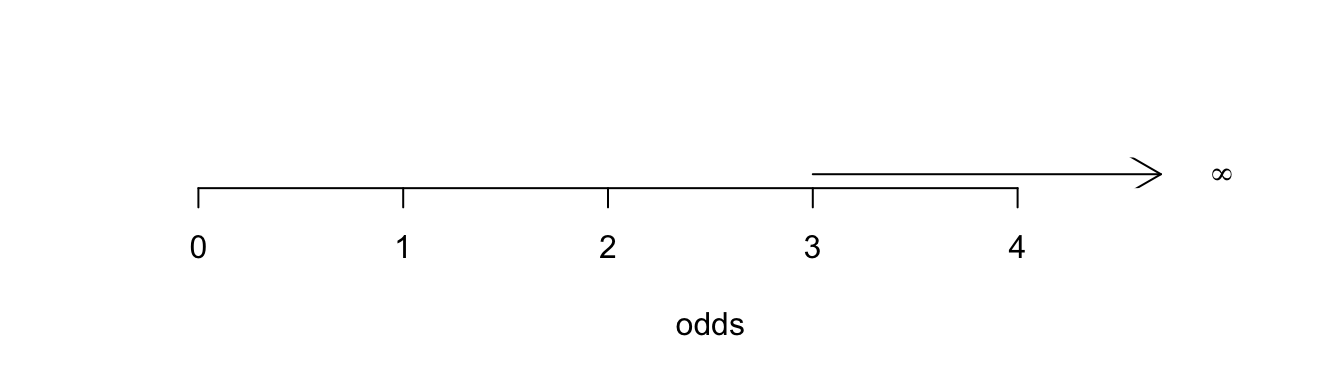
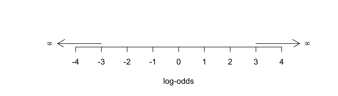
The three different scales are illustrated below. A probability close to 0 is equivalent to a log-odds close to \(-\infty\), and a probability close to 1 is equivalent to a log-odds close to \(+\infty\). A probability of 0.5 is equivalent to a log-odds of 0.
The transformation of a probability into log-odds, by first calculating odds and then taking the natural logarithm, is called the so-called logit function:
\[\texttt{logit}(p) = \ln \frac{p}{1-p}\]
This logit function is plotted in Figure 15.7.
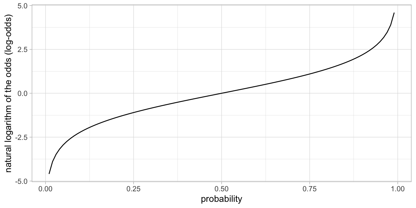
Figure 15.7: The logit function transforms probabilities into log-ods.
Because log-odds can be any value between \(-\infty\) and \(+\infty\), they are very useful for linear equations. It is therefore in logistic regression that instead of probabilities we have a linear equation for the log-odds.
15.5 Logistic link function
In previous pages we have seen that log-odds have the nice property of having meaningful values between \(-\infty\) and \(+\infty\). This makes them suitable for linear models. In essence, our linear model for our test data in children might then look like this:
\[\begin{aligned} \texttt{log-odds}_{pass}&= b_0 + b_1 \texttt{age}\\ Y &\sim Bern(p_{pass})\end{aligned}\]
Note the strange relationship between the probability parameter \(p_{pass}\) for the Bernoulli distribution, and the dependent variable for the linear equation \(\texttt{log-odds}\). The linear model predicts the log-odds, but for the Bernoulli distribution, we use the probability.
Note that earlier, we learned how a probability can be transformed into a log-odds using the logit function \(\texttt{log-odds} = \ln \frac{p}{1-p}\). We also need a way to translate the log-odds that we compute using the linear equation back into probabilities. For that we use the so-called logistic function.
\[p = \frac{e^{\texttt{log-odds}}}{1+ e^{\texttt{log-odds}}}\]
Here we see Euler’s number \(e\) again. As \(e^x\) can also be written as \(\exp(x)\), we can therefore write
\[p = \frac{\exp(\texttt{log-odds})}{1+ \exp(\texttt{log-odds})}\]
The logistic function is plotted in Figure 15.8. Its shape is S-like and resembles the cumulative normal distribution closely (see Ch. 1).
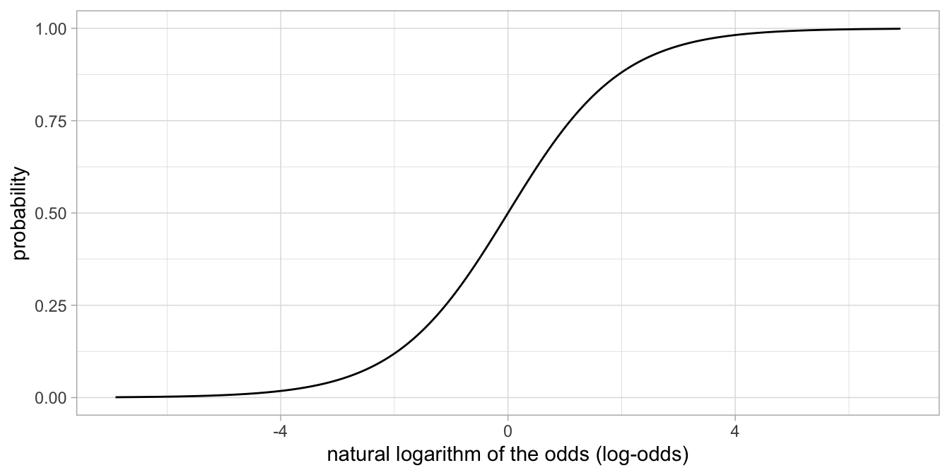
Figure 15.8: The relationship between the natural logarithm of the odds and the probability.
Overview probabilities, odds and log-odds
From probability \(p\) to odds, use
\[\begin{equation} \texttt{odds} = \frac{p}{1-p} \end{equation}\]
From probability to log-odds, use the logit function:
\[\begin{equation} \texttt{log-odds} = \textrm{logit}(p) = \textrm{ln} \frac{p}{1-p} \end{equation}\]
From log-odds to back to \(p\), use the logistic function:
\[\begin{equation} p = \frac{\textrm{exp}(\texttt{log-odds})}{1+ \textrm{exp}(\texttt{log-odds})} \end{equation}\]
15.6 Logistic regression applied to example data
So what does it look like, a linear model for log-odds?
In Figure 15.9 we show the linear model for the log-odds of passing the test for the first-graders. These log-odds are predicted by age using a straight, linear regression line.
## Warning in geom_label(aes(x = 80, y = -1), col = "black", label = "intercept: -35.75, slope: 0.46", : All aesthetics have length 1, but the data has 19 rows.
## ℹ Please consider using `annotate()` or provide this layer with data containing
##   a single row.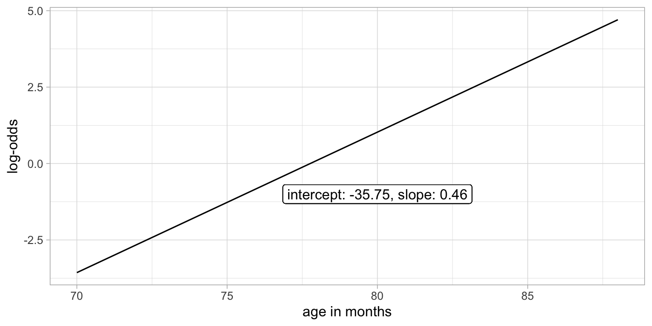
Figure 15.9: Example of a linear model for the log-odds of passing the test.
When we take all these predicted log-odds and convert them back into probabilities using the logistic function, we obtain the plot in Figure 15.10.
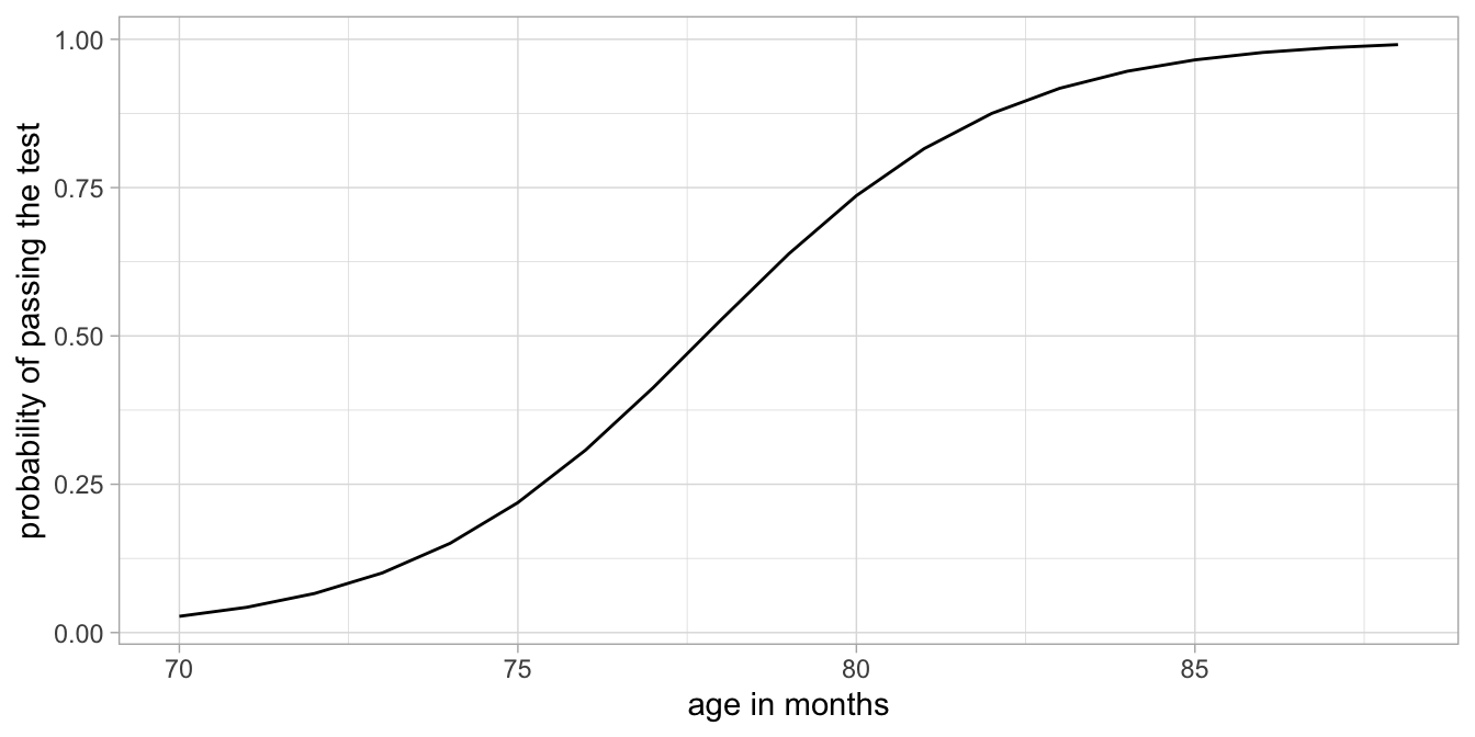
Figure 15.10: Example with log-odds transformed into probabilties (vertical axis).
Here we see an S-shape relationship between age and the probability. It has the same shape as the logistic function in Figure 15.8. We see that our model predicts probabilities close to 0 for very young ages, and probabilities close to 1 for relatively old ages. There is a clear positive effect of age on the probability of passing the test. Note that the relationship is not linear on the scale of the probabilities, see Figure 15.10, but linear on the scale of the logit of the probabilities (the log-odds), see Figure 15.9.
The curvilinear shape we see in Figure 15.10 is a logistic function of age and can be described as:
\[\begin{align} p = \textrm{logistic}(b_0 + b_1 \texttt{age}) &= \frac{\textrm{exp}(b_0 + b_1 \texttt{age})}{1+\textrm{exp}(b_0+ b_1 \texttt{age})} \\ &= \frac{\textrm{exp}(-35.75 + 0.46 \times \texttt{age})}{1+\textrm{exp}(-35.75+ 0.46 \times \texttt{age})} \end{align}\]
In summary, if we go from log-odds to probabilities, we use the logistic function, \(\textrm{logistic}(x)=\frac{\textrm{exp}(x)}{1+\textrm{exp}(x)}\). If we go from probabilities to log-odds, we use the logit function, \(\textrm{logit}(p)=\textrm{ln}\frac{p}{1-p}\). The logistic regression model is a generalised linear model with a logit link function, because the linear equation \(b_0 + b_1 X\) predicts the logit of a probability. It is also often said that we’re dealing with a logistic link function, because the linear equation gives a value that we have to subject to the logistic function to get the probability. Both terms, logit link function and logistic link function are used.
If we go back to our data on the first-grade children that either passed or failed the test, we see that this curve gives a description of our data, see Figure 15.11. The model predicts that around the age of 78 months, the probability of passing the test is around 0.50. We indeed see in Figure 15.11 that around this age about as many children pass the test (score = 1) as children that don’t (score = 0). We see that for younger ages, say around the age of 72 months, more children fail the test than pass the test. This fits with a lower probability of passing the test for such an age. For older children, say around 84 months, we see more children passing the test than failing the test, again in line with the predicted high probability.
On the basis of this analysis there seems to be a positive relationship between age in first-grade children and the probability of passing the test in this sample.
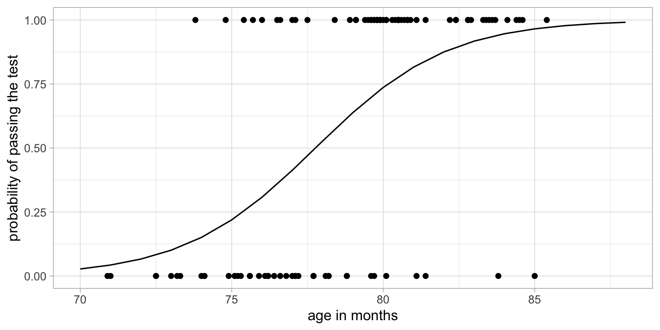
Figure 15.11: Transformed regression line and raw data points.
What we have done here is a logistic regression of passing the test on age. It is called logistic because the curve in Figure 15.11 has a logistic shape. Logistic regression is one specific form of a generalised linear model. Logistic regression is a generalised linear model with a Bernoulli distribution and a so-called logit link function: instead of modelling the probability directly, we have modelled the logit of the probabilities of obtaining a \(Y\)-value of 1 (the log-odds).
Overview
- In a regular linear model for continuous outcomes, an equation gives the predicted \(Y\)-value, and the observed \(Y\)-values are normally distributed around \(\hat{Y}\).
- For dependent variables that have only two possible outcomes, usually a Bernoulli distribution is used instead of a normal distribution.
- The probability cannot be modelled with an equation directly because probability values need to be between 0 and 1.
- Instead of the probablity \(p\), a transformation of the probability is used: the natural logarithm of the odds, also called the logit function \(\texttt{log-odds} = \textrm{logit}(p) = \textrm{ln}\frac{p}{1-p}\). We then get the equation:
\[\begin{aligned} \texttt{log-odds} = b_0 + b_1 X_1 + b_2 X_2 \end{aligned}\]
- A link is needed between the log-odds that is predicted by the equation and the probability \(p\) for the Bernoulli distribution \(Y \sim Bern(p)\). For that we use a logistic transformation:
\[\begin{equation} p = \frac{\textrm{exp}(\texttt{log-odds})}{1+ \textrm{exp}(\texttt{log-odds})} \end{equation}\]
In the next section we will see how logistic regression can be performed in R, and how we should interpret the output.
The linear model model as a special case
The regular linear model can be seen as a generalised linear model. Any generalised model has three ingredients:
- a linear equation to model predictions,
- a distribution for the actual observed outcome,
- a link function between what is predicted and the distribution.
For logistic regression we have a linear equation that predicts log-odds, and we have a Bernoulli distribution with a logit link function between the log-odds and the \(p\)-parameter of the Bernoulli distribution. For the regular linear model, we have a linear equation that gives us \(\hat{Y}\), and we use a normal distribution \(N(\hat{Y}, \sigma^2)\). Since both the equation and the distribution refer to the same \(\hat{Y}\), the link is very simple: the link function is \(\hat{Y} = \hat{Y}\). This is referred to as an identity link function ( \(\hat{Y}\) is identical to \(\hat{Y}\)). The regular linear models from previous chapters are therefore special cases of generalised linear models: generalised linear models with normal distributions and an identity link.
Besides the logit link function and the identity link function, there are several other link functions possible. One of them, the exponential link, we will discuss in the next chapter on generalised linear models for count data (Ch. 16). Apart from the Bernoulli distribution and the normal distribution, there are also alternatives, like the Poisson distribution, also discussed in Chapter 16.
15.7 Logistic regression in R
Let’s analyse the test results from the random sample of first-graders. We see part of the data in Table 15.2.
| result | age |
|---|---|
| pass | 80 |
| fail | 80 |
| fail | 78 |
| fail | 77 |
| pass | 80 |
| fail | 72 |
The dependent variable is result, and we want to study whether it is related to age. The dependent variable is dichotomous (two possible outcomes) so we choose logistic regression. The function that we use in R is the glm() function, which stands for Generalised Linear Model. We can use the following code:
## Error in eval(family$initialize): y values must be 0 <= y <= 1We get an error message: R tells us that our dependent variable needs to have values between 0 and 1. We therefore create a dummy variable score, that is 1 if the child passed the test, and 0 if it did not pass:
Next we run the logistic regression using the dummy variable as the outcome variable:
Note in the code that we specify that we want to use the binomial distribution with a logit link function. But why do we tell R to use a binomial distribution when actually we want to use a Bernoulli? Well, the Bernoulli distribution (one coin flip) is a special case of the binomial distribution (the distribution of several coin flips). So here we use a binomial distribution for one coin flip, which is equivalent to a Bernoulli distribution. Actually, the code can be a little bit shorter, because the logit link function is the default option with the binomial distribution:
Below, we see the parameter estimates from this generalised linear model run on the test data.
## # A tibble: 2 × 5
##   term        estimate std.error statistic    p.value
##   <chr>          <dbl>     <dbl>     <dbl>      <dbl>
## 1 (Intercept)  -35.7      7.58       -4.71 0.00000243
## 2 age            0.460    0.0968      4.75 0.00000203
The parameter estimates table from a glm() analysis looks very much
like that of the ordinary linear model and the linear mixed model. An
important difference is that the statistics shown are no longer
\(t\)-statistics, but \(z\)-statistics. This is because with logistic
models, the ratio \(b_1/SE\) does not have a \(t\)-distribution. In ordinary
linear models, the ratio \(b_1/SE\) has a \(t\)-distribution because in
linear models, the variance of the residuals, \(\sigma^2_e\), has to be
estimated (as it is unknown). If the residual variance were known,
\(b_1/SE\) would have a standard normal distribution. In logistic models,
there is no \(\sigma^2_e\) that needs to be estimated, so the ratio \(b_1/SE\) has a standard normal distribution. One could
therefore calculate a \(z\)-statistic \(z=b_1/SE\) and see whether that
value is smaller than 1.96 or larger than 1.96, if you want to test with
a Type I error rate of 0.05.
The interpretation of the slope parameters is very similar to other
linear models. Note that we have the following equation for the logistic
model:
\[\begin{aligned} \texttt{log-odds}_{\texttt{pass}} &= b_0 + b_1 \texttt{age} \nonumber \\ \texttt{score} &\sim Bern(p_{\texttt{pass}})\end{aligned}\]
If we fill in the values from the R output, we get
\[\begin{aligned} \texttt{log-odds}_{\texttt{pass}} &= -35.7 + 0.46 \times \texttt{age} \nonumber \\ \texttt{score} &\sim Bern(p_{\texttt{pass}})\end{aligned}\]
We can interpret these results by making some predictions. Imagine a child with an age of 72 months (on its sixth birthday). Then the predicted log-odds equals \(-35.7 + 0.46 \times 72 = -2.58\). When we transform the log-odds back to a probability,
## [1] 0.07043673we get \(\frac{\textrm{exp}(-2.58) } {1+ \textrm{exp}(-2.58) }= 0.07\). Note that the probability as well as the odds refer to the outcome that is coded as 1. Here we coded pass as “1” and fail as “0”.
To make predictions using this model easier, we can use the predict() function. In order to get the predicted log-odds we can use
##         1
## -2.649915
Note that the result \(-2.649915\) is different from our hand-calculated \(-2.58\). The difference is the result of the rounding in the R model output.
If we want to predict probabilities instead of the log-odds, we can use
##          1
## 0.06599423
So this model predicts that for children on their sixth birthday, about 7% will pass the test.
Now imagine a child on its seventh birthday (84 months): what does the model predict for the test result?
The predicted log-odds equals \(-35.7 + 0.46 \times 84 = 2.94\). When we transform this back to a probability, we get \(\frac{\textrm{exp}(2.94) } {1+ \textrm{exp}(2.94) }= 0.95\).
Letting R do the work for us, we get the same probability:
##         1
## 0.9461369
We observe that this model predicts that older children have a higher probability that they pass the test than younger children. Six year olds have a very low probability of only 7%, and seven year olds have a high probability of 95%.
A visualisation is often more helpful than a lot of calculations. The relationship between age and the probability of passing the test an be visualised using ggplot() and the add_predictions() function from the modelr package:
data.test %>%
  add_predictions(model.test, type = "response") %>%
  ggplot(aes(x = age, y = pred)) +
  geom_line() +
  geom_point(aes(y = score)) # show data points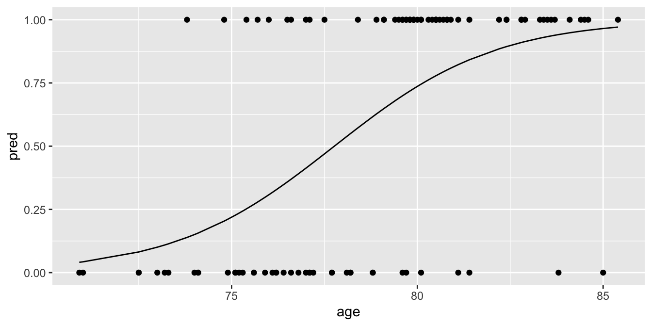
We found that the probability of passing the test is related to age in this data set of randomly selected children, but is there also an effect of age in the entire population of first-graders? The regression table shows us that the effect of age, \(+ 0.46\), is statistically significant at an \(\alpha\) of 5%, \(z = 4.75, p = .00000203\).
"In a logistic regression with dependent variable passing the test and independent variable age, the null-hypothesis was tested that age is not related to passing the test. Results showed that the null-hypothesis could be rejected, \(b_{age} = 0.46, z = 4.75, p < 0.001\). We conclude that in the population of first graders, a higher age is associated with a higher probability of passing the test."
Note that similar to other linear models, the intercept can be interpreted as the predicted log-odds for children that have values 0 for all other variables in the model. Therefore, an intercept of \(-35.7\) means in this case that the predicted log-odds for children with age 0 months equals \(-35.7\). This is equivalent to a probability of \(\frac{\textrm{exp}(-35.7) } {1+ \textrm{exp}(-35.7) }\approx 0\).
15.8 Take-away points
Logistic regression is in place when the dependent variable is dichotomous (yes/no, 1/0, TRUE/FALSE).
Logistic regression is a form of a generalised linear model.
Any generalised model has three properties: 1) a linear equation to model predictions, 2) a distribution for the actual observed outcome, and 3) a link function between what is predicted and the distribution.
In a regular linear model for continuous outcomes, an equation gives the predicted \(Y\)-value, and the observed \(Y\)-values are normally distributed around \(\hat{Y}\).
For dependent variables that have only two possible outcomes, usually a Bernoulli distribution is used instead of a normal distribution. A Bernoulli distribution depends on probability \(p\).
The probability cannot be modelled with an equation directly because the values need to be between 0 and 1.
Instead of the probablity \(p\), a transformation of the probability is used, the natural log of the odds: \(\texttt{log-odds} = \textrm{ln}\frac{p}{1-p}\). This is called the logit function. We then get the equation:
\[\texttt{log-odds} = b_0 + b_1 \texttt{X}\]
- A link is needed between the log-odds that is predicted by the equation and the probability \(p\) for the Bernoulli distribution. We call that the logit link function. We can transform a log-odds into a probability using the logistic function:
\[p = \frac{\textrm{exp}(\texttt{log-odds})}{1+ \textrm{exp}(\texttt{log-odds})}\]