Chapter 14 Non-parametric alternatives for linear mixed models
14.1 Checking assumptions
In previous chapters we discussed the assumptions of linear models and linear mixed models: linearity (in parameters), homoscedasticity (equal variance), normal distribution of residuals, normal distribution of random effects (relevant for linear mixed models only), and independence (no clustering unaccounted for).
The problem of non-linearity can sometimes be solved by introducing quadratic terms, by replacing a linear model \(Y = b_0 + b_1 X + e\) by another linear model \(Y = b_0 + b_1 X + b_2 X^2 + e\).
If we have non-independence, then you can introduce either an extra fixed effect or a random effect for a clustering variable. For example, if you see that cars owned by low income families have much more mileage than cars owned by high income families, you can account for this by adding a fixed effect of an income variable as predictor. If you see that average mileage is rather similar within municipality but that average mileage can vary quite a lot across municipalities, you can introduce a random effect for municipality (if you have data say from 30 different municipalities).
Unequal variance of residuals and non-normal distribution of residuals are harder to tackle. Non-normality can sometimes be solved by using generalised linear models (see Chapter 15). A combination of non-normality and unequal variance can sometimes be easily solved by using a transformation of the dependent variable, for instance not analysing \(Y = b_0 + b_1 X + e\) but analysing \(\textrm{log}(Y)= b_0 + b_1 X + e\) or \(\sqrt{Y}= b_0 + b_1 X + e\). There are also more advanced options available that will not be discussed here but that make corrections to standard errors and \(p\)-values that render inference more robust against model violations.
If these data transformations or advanced options don’t work (or if
you’re not acquainted with them), and your data show non-equal variance
and/or non-normally distributed residuals, there are non-parametric
alternatives. Here we discuss two: Friedman’s test and Wilcoxon’s signed
rank test. We explain them using an imaginary data set on speed
skating.
Suppose we have data on 12 speed skaters that participate on the 10
kilometres distance in three separate championships in 2017-2018: the
European Championships, the Winter Olympics and the World Championships.
Your friend expects that speed skaters will perform best at the Olympic
games, so there she expects the fastest times. You disagree and decide
to test the null-hypothesis that average times are the same at the three
occasions. You regard the data from 2017-2018 to be a random sample of
all seasons in the past and future. In Figure
14.1 we see a boxplot of the data.
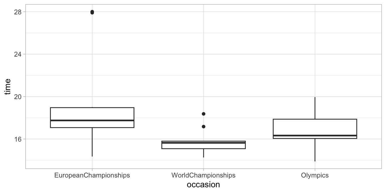
Figure 14.1: Boxplot of the imaginary speed skating data.
In order to test your null-hypothesis, we run a linear mixed model with
dependent variable time, and independent variable occasion. We use
random effects for the differences in speed across skaters. In Figure
14.2 we see the residuals. From this plot we
clearly see that the assumption of equal variance (homogeneity of
variance) is violated: the variance of the residuals in the World
Championships condition is clearly smaller than the variance of the
European Championships condition. From the histogram of the residuals in
Figure 14.3 we also see that the distribution of the
residuals is not bell-shaped: it is positively skewed (skewed to the
right).
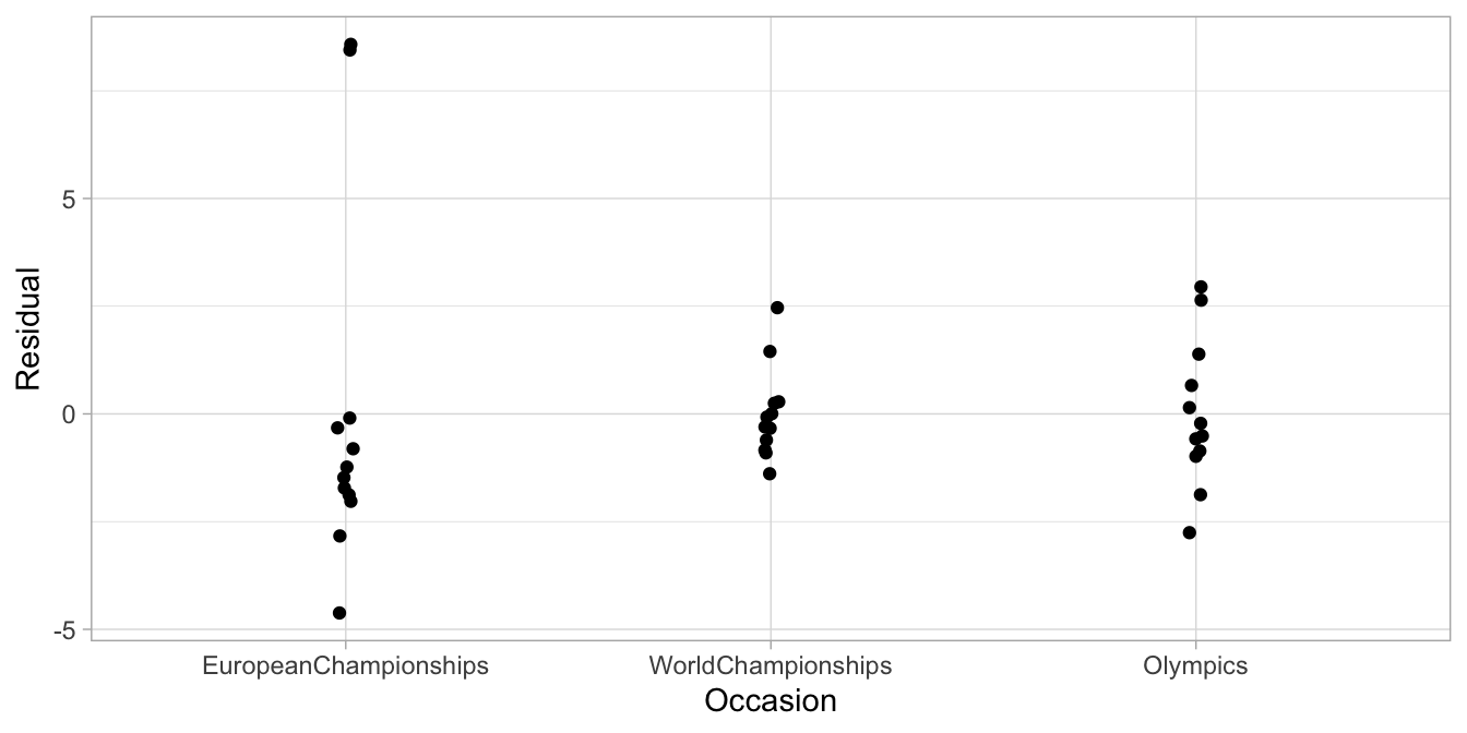
Figure 14.2: Residuals of the speedskating data with a linear mixed model.
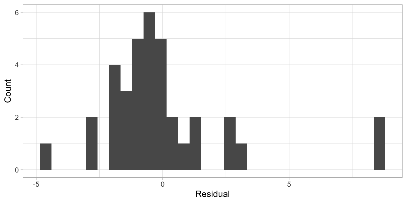
Figure 14.3: Histogram of the residuals of the speedskating data with a linear mixed model.
Since the assumptions of homogeneity of variance and of normally distributed residuals are violated23, the results from the linear mixed model cannot be trusted. In order to answer our research question, we therefore have to resort to another kind of test. Here we discuss Friedman’s test, a non-parametric test, for testing the null-hypothesis that the medians of the three groups of data are the same (see Chapter 1). This Friedman test can be used in all situations where you have at least 2 levels of the within variable. In other words, you can use this test when you have data from three occasions, but also when you have data from 10 occasions or only 2. In a later section the Wilcoxon signed ranks test is discussed. This test is often used in social and behavioural sciences. The downside of Wilcoxon’s test is that it can only handle data sets with 2 levels of the within variable. In other words, it can only be used when we have data from two occasions. Friedman’s test is therefore more generally applicable than Wilcoxon’s.
14.2 Friedman’s test for \(k\) measures
Similar to many other non-parametric tests for testing the equality of medians, Friedman’s test is based on ranks. Table 14.1 shows the speed skating data in wide format.
| athlete | EuropeanChampionships | WorldChampionships | Olympics |
|---|---|---|---|
| 1 | 14.35 | 15.79 | 16.42 |
| 2 | 17.36 | 14.26 | 18.13 |
| 3 | 19.01 | 18.37 | 19.95 |
| 4 | 27.90 | 15.12 | 17.78 |
| 5 | 17.67 | 17.17 | 16.96 |
| 6 | 17.83 | 15.30 | 16.15 |
| 7 | 16.30 | 15.63 | 19.44 |
| 8 | 28.00 | 15.69 | 16.23 |
| 9 | 18.27 | 15.65 | 15.76 |
| 10 | 17.00 | 14.99 | 16.18 |
| 11 | 17.10 | 15.83 | 13.89 |
| 12 | 18.94 | 14.77 | 14.83 |
We rank all of these time measures by determining the fastest time, then the next to fastest time, etcetera, until the slowest time. But because the data in each row belong together (we compare individuals with themselves), we do the ranking row-wise. For each athlete separately, we determine the fastest time (1), the next fastest time (2), and the slowest time (3) and put the ranks in a new table, see Table 14.3. There we see for example that athlete 1 had the fastest time at the European Championships (14.35, rank 1) and the slowest at the Olympics (16.42, rank 3).
| athlete | EuropeanChampionships | WorldChampionships | Olympics |
|---|---|---|---|
| 1 | 1 | 2 | 3 |
| 2 | 2 | 1 | 3 |
| 3 | 2 | 1 | 3 |
| 4 | 3 | 1 | 2 |
| 5 | 3 | 2 | 1 |
| 6 | 3 | 1 | 2 |
| 7 | 2 | 1 | 3 |
| 8 | 3 | 1 | 2 |
| 9 | 3 | 1 | 2 |
| 10 | 3 | 1 | 2 |
| 11 | 3 | 2 | 1 |
| 12 | 3 | 1 | 2 |
Next, we compute the sum of the ranks column-wise: the sum of the ranks for the European Championships data is 31, for the Olympic data it’s 15 and for the World Championships data it is 26. We call these sums \(S_j\), where the \(j\) indicates the column.
From these sums \(S_j\) we can gather that in general, these athletes showed their best times (many rank 1s) at the World Championships, as the sum of the ranks is lowest. We also see that in general these athletes showed their worst times (many rank 2s and 3s) at the European Championships, as the relevant column showed the highest sum of ranks.
In order to know whether these sums of ranks are significantly different from each other, we may compute an \(F_r\)-value based on the following formula:
\[F_r = \left[ \frac{12}{nk(k+1)} \Sigma^k_{j=1} S_j^2 \right] - 3n (k+1)\]
In this formula, \(n\) stands for the number of rows (12 athletes), \(k\) stands for the number of columns (3 occasions), and \(S_j^2\) stands for the squared sum of column \(j\) (\(31^2\), \(15^2\), and \(26^2\), respectively). If we fill in these numbers, we get:
\[\begin{aligned} F_r &= \left[ \frac{12}{12 \times 3(3+1)} \times (31^2 + 15^2 + 26^2) \right] - 3 \times 12 (3+1) \nonumber \\ &= \left[ \frac{12}{144} \times 1862 \right] - 144 = 11.167 \nonumber\end{aligned}\]
What can we tell from this \(F_r\)-statistic? In order to say something about significance, we have to know what values are to be expected under the null-hypothesis that there are no differences across the three groups of data. Suppose we randomly mixed up the data by taking all the speed skating times and randomly assigning them to the three contests and the twelve athletes, until we have a newly filled data matrix, for example the one in Table 14.5.
| athlete | EuropeanChampionships | WorldChampionships | Olympics |
|---|---|---|---|
| 1 | 15.76 | 14.26 | 17.78 |
| 2 | 19.44 | 17.10 | 17.83 |
| 3 | 16.18 | 14.83 | 15.63 |
| 4 | 15.30 | 17.00 | 16.42 |
| 5 | 15.79 | 16.23 | 17.36 |
| 6 | 14.77 | 28.00 | 15.65 |
| 7 | 14.35 | 16.15 | 16.30 |
| 8 | 27.90 | 15.12 | 18.94 |
| 9 | 16.96 | 19.01 | 19.95 |
| 10 | 15.83 | 17.17 | 13.89 |
| 11 | 14.99 | 18.27 | 15.69 |
| 12 | 18.37 | 17.67 | 18.13 |
If we then compute \(F_r\) for this data matrix, we get a different value. If we do this mixing up the data and computing \(F_r\) say 1000 times, we get 1000 values for \(F_r\), summarised in the histogram in Figure 14.4.
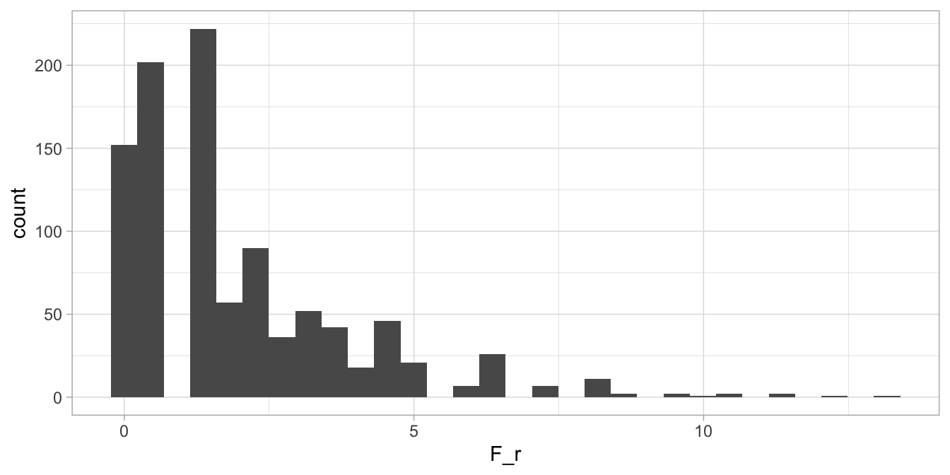
Figure 14.4: Histogram of 1000 possible values for \(F_r\) given that the null-hypothesis is true, for 12 speed skaters.
So if the data are just randomly distributed over the three columns (and 12 rows) in the data matrix, we expect no systematic differences across the three columns and so the null-hypothesis is true. So now we know what the distribution of \(F_r\) looks like when the null-hypothesis is true: more or less like the one in Figure 14.4. Remember that for the true data that we actually gathered (in the right order that is!), we found an \(F_r\)-value of 11.167 . From the histogram, we see that only very few values of 11.167 or larger are observed when the null-hypothesis is true. If we look more closely, we find that only 0.2% of the values are larger than 11.167 , so we have a two-tailed \(p\)-value of 0.004. The 95th percentile of these 1000 \(F_r\)-values is 6.1666667, meaning that of the 1000 values for \(F_r\), 5% are larger than 6.1666667. So if we use a significance level of 5%, our observed value of 11.167 is larger than the critical value for \(F_r\), and we conclude that the null-hypothesis can be rejected.
Now this \(p\)-value of 0.004 and the critical value of 6.1666667 are based on our own computations24. Actually there are better ways. One is to look up critical values of \(F_r\) in tables, for instance in Kendall M.G. (1970) Rank correlation methods. (fourth edition). The \(p\)-value corresponding to this \(F_r\)-value depends on \(k\), the number of groups of data (here 3 columns) and \(n\), the number of rows (12 individuals). If we look up that table, we find that for \(k=3\) and \(n=12\) the critical value of \(F_r\) for a type I error rate of 0.05 equals 6.17. Our observed \(F_r\)-value of 11.167 is larger than that, therefore we can reject the null-hypothesis that the median skating times are the same at the three different championships. So we have to tell your friend that there are general differences in skating times at different contests, \(F_r=11.167 , p < 0.05\), but it is not the case that the fastest times were observed at the Olympics.
A third way to do null-hypothesis testing is to make an approximation of the distribution of \(F_r\) under the null-hypothesis. Note that the distribution in the histogram in Figure 14.4 is very strangely shaped. The reason is that the data set is quite limited. Suppose we have data not on 12 speed skaters, but on 120. If we then randomly mix up data again and compute 1000 different values for \(F_r\), we get the histogram in Figure 14.5.
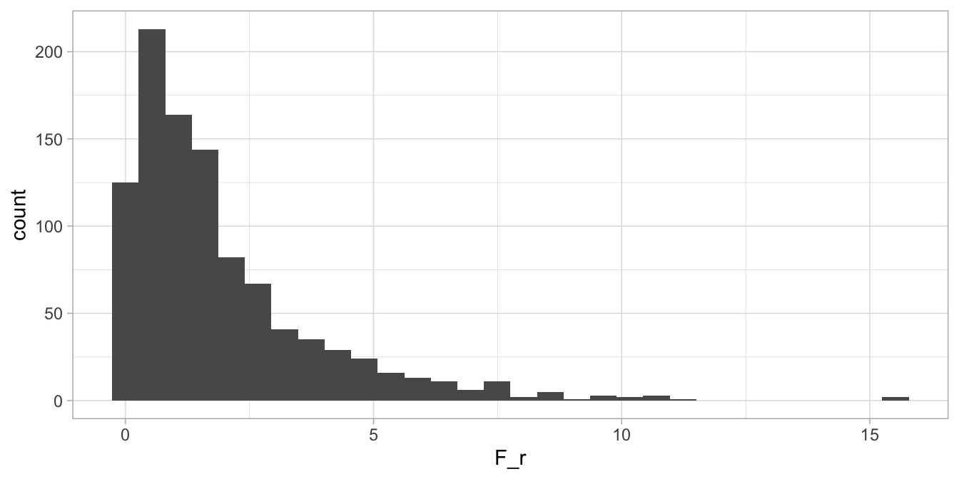
Figure 14.5: Histogram of 1000 possible values for \(F_r\) given that the null-hypothesis is true, for 120 speed skaters.
The shape becomes more regular. It also starts to resemble another distribution, that of the \(\chi^2\) (chi-square). It can be shown that the distribution of the \(F_r\) for a large number of rows in the data matrix, and at least 6 columns, approaches the shape of the \(\chi^2\)-distribution with \(k-1\) degrees of freedom. This is shown in Figure 14.6.
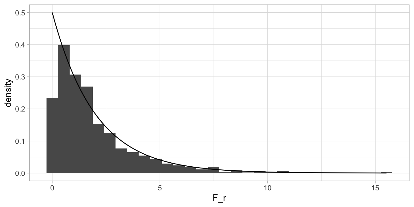
Figure 14.6: The distribution of \(F_r\) under the null-hypothesis, overlain with a chi-square distribution with 2 degrees of freedom.
The density of the \(\chi^2\)-distribution with 2 degrees of freedom approaches the histogram quite well, but not perfectly. In general, for large \(n\) and \(k>5\), the approximation is very good. In that way it gets easier to look up \(p\)-values for certain \(F_r\)-values, because the \(\chi^2\)-distribution is well-known25, so we don’t have to look up critical values for \(F_r\) in old tables. For a significance level of 5%, the critical value of a \(\chi^2\) with 2 degrees of freedom is 5.991. We can see that in R with the following code:
# critical value for chi-square distribution
# with 2 degrees of freedom and alpha = 0.05:
qchisq(p = 0.95, df = 2)
## [1] 5.991465This is close to the value in the table for \(F_r\) in old books: 6.17. The part of the \(\chi^2\)-distribution with 2 degrees of freedom that is larger than the observed 11.167 is 0.004, so our approximate \(p\)-value for our null-hypothesis is 0.004.
# p-value for statistic of 11.167 based on
# chi-square distribution with 2 degrees of freedom:
pchisq(11.167, df = 2, lower.tail = F)
## [1] 0.00375938514.3 Comparing Friedman’s test with linear mixed model on ranks (advanced)
Remember that for many non-parametric tests, they are equivalent to applying a linear model on ranks. This is not true for this Friedman test. For this data set, we could ignore potential problems with the data and carry out a linear mixed model analysis, using the actual finishing times, and predict them with a fixed effect for the type of championship and a random effect for each individual skater. If you have doubts about the assumptions, apply a non-parametric test like the Friedman test.
Alternatively, we could apply ranking on all the finish times, not row-wise as we do for Friedman’s test but lumping all times together. Next, we apply the same linear mixed model analysis with a fixed effect for the type of championship and a random effect the skaters, now using the ranks as dependent variable. The result would be a perfectly acceptable analysis, however, it is not equivalent to Friedman’s test.26
14.4 How to perform Friedman’s test in R
In order to let R do the calculations for you, you need first of all
your data to be in long format. If your data happen to be in wide
format, use the pivot_longer() function to get the data in long
format. Suppose your data is in wide format, as in Table
14.1. Then the following code turns the data
into long format:
This creates the long format data matrix in Table 14.7:
| athlete | occasion | time |
|---|---|---|
| 1 | EuropeanChampionships | 14.35 |
| 1 | Olympics | 16.42 |
| 1 | WorldChampionships | 15.79 |
| 2 | EuropeanChampionships | 17.36 |
| 2 | Olympics | 18.13 |
| 2 | WorldChampionships | 14.26 |
We can then specify that we want Friedman’s test by using the
friedman.test() function and indicating which variables we want to
use:
##
##  Friedman rank sum test
##
## data:  time and occasion and athlete
## Friedman chi-squared = 11.167, df = 2, p-value = 0.00376
This code says, "use time as dependent variable, occasion as
independent variable, and the data are clustered within athletes (data
with the same athlete ID number belong together)".
In the output we see a chi-squared statistic, degrees of freedom, and an asymptotic (approximated) \(p\)-value. Why don’t we see an \(F_r\)-statistic?
The reason is, as discussed in the previous section, that for a large number of measurements (in wide format: columns) and a large number of individuals (in wide format: rows), the \(F_r\) statistic tends to have the same distribution as a chi-square, \(\chi^2\), with \(k-1\) degrees of freedom. So what we are looking at in this output is really an \(F_r\)-value of 11.167 (exactly the same value as we computed by hand in the previous section). In order to approximate the \(p\)-value, this value of 11.167 is interpreted as a chi-square (\(\chi^2\)), which with 2 degrees of freedom has a \(p\)-value of 0.004.
This asymptotic (approximated) \(p\)-value is the correct \(p\)-value if you have a lot of rows (large \(n\)) and at least 6 variables (\(k>5\)). If you do not have that, as we have here, this asymptotic \(p\)-value is only what it is: an approximation. However, this is only a problem when the approximate \(p\)-value is close to the pre-selected significance level \(\alpha\). If \(\alpha\) equals 0.05, an approximate \(p\)-value of 0.002 is much smaller than that, and we do not hesitate to call it significant, whatever its true value may be. If a \(p\)-value is very close to \(\alpha\), it might be a good idea to look up the exact critical values for \(F_r\) in online tables27. If your \(F_r\) is larger than the critical value for a certain combination of \(n\), \(k\) and \(\alpha\), you may reject the null-hypothesis.
In the above case we can report:
"A Friedman’s test showed that speed skaters have significantly different median times on the 10 kilometre distance at the three types of contests, \(F_r = 11.167 , p = .004\)."
Linear mixed model version on rank data
Althought it is not equivalent to Friedman’s test, the same data could be analysed using a linear mixed model on the ranks. We start from the long data format with the original data and create new variable for the ranks:
##   athlete              occasion  time rank
## 1       1 EuropeanChampionships 14.35    3
## 2       1              Olympics 16.42   19
## 3       1    WorldChampionships 15.79   13
## 4       2 EuropeanChampionships 17.36   24
## 5       2              Olympics 18.13   28
## 6       2    WorldChampionships 14.26    2
Note that we now have large values for the ranks: the data is ranked across all skaters and all championships, in contrast to Friedman’s test where the ranking is done within individual skaters.
Next we apply a linear mixed model and ask for an ANOVA, testing the null-hypothesis that the three championships show the same average rank in the population.
library(lmerTest)
library(car)
datalong %>%
  lmer(rank ~ occasion + (1|athlete), data = .) %>%
  Anova(type = 3, test.statistic = "F")
## Analysis of Deviance Table (Type III Wald F tests with Kenward-Roger df)
##
## Response: rank
## F Df Df.res Pr(>F)
## (Intercept) 92.3181 1 32.409 5.246e-11 ***
## occasion 7.6717 2 22.000 0.002967 **
## ---
## Signif. codes: 0 '***' 0.001 '**' 0.01 '*' 0.05 '.' 0.1 ' ' 1We can report:
"A linear mixed model on the ranked times showed that speed skaters have significantly different median times on the 10 kilometre distance across the three types of contests, \(F(2, 22) = 7.67 , p = .003\)."
14.5 Wilcoxon’s signed ranks test for 2 measures
Friedman’s test can be used for 2 measures, 3 measures or even 10
measures. As stated earlier, the well-known Wilcoxon’s test can only be
used for 2 measures. For completeness, we also discuss that test here.
For that test we compare the measures at the Olympics and at the World
Championships.
For each athlete, we take the difference in skating times (Olympics -
WorldChampionships) and call it \(d\), see Table
14.9. Next we rank these \(d\)-values,
irrespective of sign, and call these ranks rank_d. From Table
14.9 we see that athlete 12 shows the
smallest difference in skating times (\(d = 0.06\), rank = 1) and athlete
2 the largest difference (\(d= 3.78\), rank = 12).
| athlete | WorldChampionships | Olympics | d | rank_d | ranksign |
|---|---|---|---|---|---|
| 1 | 15.79 | 16.42 | 0.63 | 5 | 5 |
| 2 | 14.26 | 18.13 | 3.87 | 12 | 12 |
| 3 | 18.37 | 19.95 | 1.58 | 8 | 8 |
| 4 | 15.12 | 17.78 | 2.66 | 10 | 10 |
| 5 | 17.17 | 16.96 | -0.21 | 3 | -3 |
| 6 | 15.30 | 16.15 | 0.85 | 6 | 6 |
| 7 | 15.63 | 19.44 | 3.81 | 11 | 11 |
| 8 | 15.69 | 16.23 | 0.54 | 4 | 4 |
| 9 | 15.65 | 15.76 | 0.11 | 2 | 2 |
| 10 | 14.99 | 16.18 | 1.19 | 7 | 7 |
| 11 | 15.83 | 13.89 | -1.94 | 9 | -9 |
| 12 | 14.77 | 14.83 | 0.06 | 1 | 1 |
Next, we indicate for each rank whether it belongs to a positive or a
negative difference \(d\) and call that variable ranksign.
Under the null-hypothesis, we expect that some of the larger \(d\)-values are positive and some of them negative, in a fairly equal amount. If we sum the ranks having plus-signs and sum the ranks having minus-signs, we would expect that these two sums are about equal, but only if the null-hypothesis is true. If the sums are very different, then we should reject this null-hypothesis. In order to see if the difference in sums is too large, we compute them as follows:
\[\begin{aligned} T^+ &= 5+ 12 + 8 +10+6+11+4 +2 +7 +1 = 66 \nonumber \\ T^- &= 3 + 9= 12 \nonumber\end{aligned}\]
To know whether \(T^+\) is significantly larger than \(T^-\), the value of \(T^+\) can be looked up in a table, for instance in Siegel & Castellan (1988). There we see that for \(T^+\), with 12 rows, the probability of obtaining a \(T^+\) of at least 66 is 0.0171. For a two-sided test (if we would have switched the columns of the two championships, we would have gotten a \(T^-\) of 66 and a \(T^+\) of 12!), we have to double this probability. So we end up with a \(p\)-value of \(2 \times 0.0171=0.0342\).
In the table we find no critical values for large sample size \(n\), but fortunately, similar to the Friedman test, we can use an approximation using a different distribution, here the normal distribution. It can be shown that for large sample sizes, the statistic \(T^+\) is approximately normally distributed with mean
\[\mu = \frac{n(n+1)}{4}\]
and variance:
\[\sigma^2= \frac {n(n+1)(2n+1) } {24}\]
If we therefore standardise the \(T^+\) by subtracting the \(\mu\) and then dividing by the square root of the variance \(\sqrt(\sigma^2)=\sigma\), we get a \(z\)-value with mean 0 and standard deviation 1. To do that, we use the following formula:
\[z = \frac{T^+ - \mu}{\sigma} = \frac { T^+ - n(n+1)/4} {\sqrt{n(n+1)(2n+1)/24}}\]
Here \(T^+\) is 66 and \(n\) equals 12, so if we fill in the formula we get \(z = 2.118\). From the standard normal distribution we know that 5% of the observations lie above 1.96 and below -1.96. So a value for \(z\) larger than 1.96 or smaller than -1.96 is enough evidence to reject the null-hypothesis. Here our \(z\)-statistic is larger than 1.96, therefore we reject the null-hypothesis that the median skating times are the same at the World Championships and the Olympics. The \(p\)-value associated with a \(z\)-score of 2.118 is 0.034.
The analysis for a Wilcoxon test looks complicated, but is actually equivalent to a linear mixed model applied to ranked data for moderate to large data sets.28 This will be further discussed at the end of the next section.
14.6 How to perform Wilcoxon’s signed ranks test in R
If you want R to perform the Wilcoxon test, your data needs to be in
wide format. If your data are in long format, you can transform them
with the function pivot_wider():
datawide <- datalong %>%
  pivot_wider(id_cols = athlete, values_from = "time", names_from = "occasion")
Next, you use the wilcox.test() function. You select the two
variables (occasions) that you would like to compare, and indicate that
the Olympic and World Championship data are paired within rows (i.e.,
the Olympic and World championship data in one row belong to the same
individual).
##
##  Wilcoxon signed rank exact test
##
## data:  datawide$Olympics and datawide$WorldChampionships
## V = 66, p-value = 0.03418
## alternative hypothesis: true location shift is not equal to 0
The output shows a \(V\)-statistic, which corresponds to our \(T^+\) above.
The standard output yields an approximate \(p\)-value. This \(p\)-value is
by default two-sided. Wilcoxon’s \(T^+\)-statistic (or \(V\)) under the
null-hypothesis approaches a normal distribution in case we have a large
number of observations (many rows in wide format). If \(n>15\), the
approximation is good enough so that if we standardise this statistic,
it can be interpreted as a \(z\)-score (standardised score with a normal
distribution). That means that a \(z\)-score of 1.96 or larger or -1.96 or
smaller can be regarded as significant at the 5% significance level.
Since the standard normal distribution is only an approximation, and we
have \(n=12\), it is safer here to look at the exact significance level.
That can be done with the option exact = TRUE:
##
##  Wilcoxon signed rank exact test
##
## data:  datawide$Olympics and datawide$WorldChampionships
## V = 66, p-value = 0.03418
## alternative hypothesis: true location shift is not equal to 0
In this case we see that the exact \(p\)-value is equal, to the fifth
decimal, to the approximate \(p\)-value. Note that we use a two-sided
test, to allow for the fact that random sampling could lead to a higher
median for the Olympic Games or a higher median for the World
Championships. We just want to know whether the null-hypothesis that the
two medians differ can be rejected (in whatever direction) or not.
Let’s compare the output with the Friedman test, but then only use the
relevant occasions in your code:
datalong %>%
  filter(occasion != "EuropeanChampionships") %>%
  mutate(occasion = as.integer(occasion)) %>%
  friedman.test(time ~ occasion | athlete,
                data = .)
##
## Friedman rank sum test
##
## data: time and occasion and athlete
## Friedman chi-squared = 5.3333, df = 1, p-value = 0.02092Note that the friedman.test() function does not perform well if some
variables are factors and you make a selection of the levels. Here we
have the factor occasion with originally 3 levels. If the
friedman.test() function only finds two of these in the data it is
supposed to analyse, it throws an error. Therefore we turn factor
variable occasion into an integer variable first. The
friedman.test() function then turns this integer variable into a new
factor variable with only 2 levels before the calculations.
In the output we see that the null-hypothesis of equal medians at the World Championships and the Olympic Games can be rejected, with an approximate \(p\)-value of 0.02.
Note that both the Friedman and Wilcoxon tests come up with very similar
\(p\)-values, even though their rationales are different: Friedman’s test is based
on ranks and Wilcoxon’s test is based on the size of positive and negative
differences between measures 1 and 2. Wilcoxon’s test therefore uses more information than Friedman’s test. Both can be used in the case you have two measures. Friedman’s test can be used in all situations where you have 2 or more measures per row, whereas Wilcoxon’s test can only be used if you have 2 measures per row.
In sum, we can report in two ways on our hypothesis regarding similar
skating times at the World Championships and at the Olympics:
"A Friedman test showed a significant difference between the 10km skating times at the World Championships and at the Olympics, \(F_r = 5.33, p = .02\)."
"A Wilcoxon signed ranks test showed a significant difference between the 10km skating times at the World Championships and at the Olympics, \(T^+ = 66, p = .03\)."
How do we know whether the fastest times were at the World Championships
or at the Olympics? If we look at the raw data in Table
14.1, it is not immediately obvious. We have
to inspect the \(T^+ = 66\) and \(T^- = 12\) and consider what they
represent: there is more positivity than negativity. The positivity is
due to positive ranksigns that are computed based on
\(d = Olympics - WorldChampionships\), see Table
14.9. A positive difference \(d\) means that
the Olympics time was larger than the WorldChampionships time. A large
value for time stands for slower speed. A positive ranksign therefore
means that the Olympics time was larger (slower!) than the
WorldChampionships time. A large rank_d means that the difference
between the two times was relatively large. Therefore, you get a large
value of \(T^+\) if the Olympic times are on the whole slower than the
World Championships times, and/or when these positive differences are
relatively large. When we look at the values of ranksign in Table
14.9, we notice that only two values are
negative: one relatively large value and one relatively small value. The
rest of the values are positive, both small and large, and these all
contribute to the \(T^+\) value. We can therefore state that the pattern
in the data is that for most athletes, the Olympic times are slower than
the times at the World Championships.
Of course, this is better visualised with a graph, see Figure 14.7. Easy to see that for 2 skaters, the times were fastest at the Olympics. The rest had their best time at the World Championships.
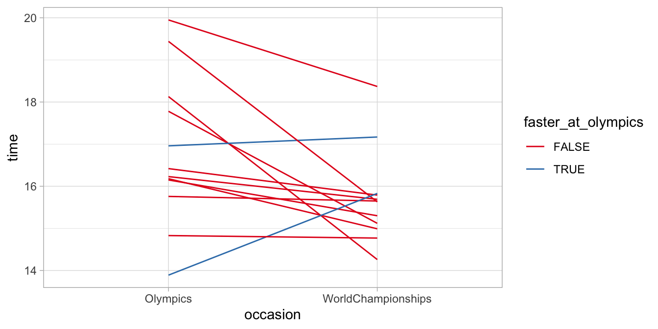
Figure 14.7: Skating times at the Olympics and the World Championships. Only two of the skaters show their fastest time at the Olympics.
Wilcoxon equals linear mixed model applied to ranks
Wilcoxon’s test can also be conceived of as the analog of a linear model on ranks. If we turn the skating data from the World Championships and the Olympic Games into ranks, we can apply a linear mixed model with a fixed effect for occasion and a random effect for the skater. In R we start from the data in long format:
library(lmerTest)
datalong %>%
  filter(occasion != "EuropeanChampionships") %>%
  mutate(rank = rank(time)) %>%
  lmer(rank ~ occasion + (1|athlete), data = .) %>%
  summary()
## Linear mixed model fit by REML. t-tests use Satterthwaite's method [
## lmerModLmerTest]
## Formula: rank ~ occasion + (1 | athlete)
## Data: .
##
## REML criterion at convergence: 149.9
##
## Scaled residuals:
## Min 1Q Median 3Q Max
## -2.11878 -0.59704 0.05797 0.78980 1.48883
##
## Random effects:
## Groups Name Variance Std.Dev.
## athlete (Intercept) 8.939 2.99
## Residual 34.576 5.88
## Number of obs: 24, groups: athlete, 12
##
## Fixed effects:
## Estimate Std. Error df t value Pr(>|t|)
## (Intercept) 9.667 1.904 21.109 5.076 4.93e-05 ***
## occasionOlympics 5.667 2.401 11.000 2.361 0.0378 *
## ---
## Signif. codes: 0 '***' 0.001 '**' 0.01 '*' 0.05 '.' 0.1 ' ' 1
##
## Correlation of Fixed Effects:
## (Intr)
## occsnOlympc -0.630From the results we see that the average rank is higher in the Olympics data. The \(p\)-value is lower than 0.05, so we conclude:
"A linear mixed model on the ranked data (Wilcoxon’s test) showed a significant difference between the 10km skating times at the World Championships and at the Olympics, \(t = 2.36, p = .04\)."
Note that the \(p\)-value is slightly different compared to the Wilcoxon test result earlier. This is because the data set is relatively small. For moderate to large sample sizes, the difference will disappear.
14.7 Ties
Many non-parametric tests are based on ranks. For example, if we have the data sequence 0.1, 0.4, 0.5, 0.2, we give these values the ranks 1, 3, 4, 2, respectively. But in many data cases, data sequences cannot be ranked unequivocally. Let’s look at the sequence 0.1, 0.4, 0.4, 0.2. Here we have 2 values that are exactly the same. We say then that we have ties. If we have ties in our data like the 0.4 in this case, one very often used option is to arbitrarily choose one of the 0.4 values as smaller than the other, and then average the ranks. Thus, we rank the data into 1, 3, 4, 2 and then average the tied observations: 1, 3.5, 3.5, 2. As another example, suppose we have the sequence 23, 54, 54, 54, 19, we turn this into ranks 2, 3, 4, 5, 1 and take the average of the ranks of the tied observations of 54: 2, 4, 4, 4, 1. These ranks corrected for ties can then be used to compute the test statistic, for instance Friedman’s \(F_r\) or Wilcoxon’s \(z\). However, in many cases, because of these corrections, a slightly different formula is to be used. So the formulas become a little bit different. This is all done in R automatically. If you want to know more, see Siegel and Castellan (1988). Non-parametric Statistics for the Behavioral Sciences. New York: McGraw-Hill.
14.8 Take-away points
When a distribution of residuals looks very far removed from a normal distribution and/or shows heterogeneity of variance, consider either a data transformation or using a non-parametric method of analysis.
Friedman’s and Wilcoxon’s tests are non-parametric alternatives for linear mixed modelling with one categorical predictor variable, in a within-subjects design.
Wilcoxon’s can be used for an independent variable with only two categories.
Friedman’s test can also be used for an independent variable with more than two categories.
Alternatively to Wilcoxon’s test and Friedman’s test, one can apply linear mixed models to ranked data. Wilcoxon’s test is actually equivalent to a linear mixed model on ranks, and will yield the same \(p\)-values for large enough samples.
Remember that assumptions relate to the population, not samples: often-times your data set is too small to say anything about assumptions at the population level. Residuals for a data set of 8 persons might show very non-normal residuals, or very different variances for two subgroups of 4 persons each, but that might just be a coincidence, a random result because of the small sample size. If in doubt, it is best to use non-parametric methods.↩︎
What we have actually done is a very simple form of bootstrapping or permutation testing: jumbling up the data set many times and in that way determining the distribution of a test-statistic under the null-hypothesis, in this case the distribution of \(F_r\). For more on bootstrapping, see Davison, A.C. & Hinkley, D.V. (1997). Bootstrap Methods and their Application. Cambridge, UK: Cambridge.↩︎
The \(\chi^2\)-distribution is based on the normal distribution: the \(\chi^2\)-distribution with \(k\) degrees of freedom is the distribution of a sum of the squares of \(k\) independent standard normal random variables.↩︎
See for instance https://seriousstats.wordpress.com/2012/02/14/friedman/↩︎
see https://seriousstats.wordpress.com/2012/02/14/friedman/↩︎