Chapter 3 Inference about a proportion
3.1 Sampling distribution of the sample proportion
So far, we focused on inference about a population mean: starting from a sample mean, what can we infer about the population mean? However, there are also other sample statistics we could focus on. We briefly touched on the variance in the sample and what it tells us about the population variance. In this section, we focus on inference regarding a proportion.
Let’s go back to the example of the elephants in the zoo, and that the manager saw a damaged doorway. This is most likely caused by elephants that are taller than a certain height, making their heads bump the doorway when moving from one space to the other. Let’s suppose the height of the doorway is 3.40 m and that the manager observes that of the 4 elephants in the zoo, 3 bump their head when passing the doorway. Suppose that the 4 elephants are randomly sampled from the entire population of elephants worldwide. What could we say based on these observations about the proportion of elephants worldwide that are taller than 3.40 m?
Let’s again start from the population. Let’s do the thought experiment that the population proportion of elephants taller than 3.40 m equals 0.6: 60% of all the elephants in the world are taller than 3.40 m. Let’s randomly pick 4 elephants from this population. We might get 2 tall elephants and 2 less tall elephants. This means we get a sample proportion of \(\frac{2}{4} = 0.5\). If we do this sampling a lot of times, we obtain the sampling distribution of the sample proportion. It is shown in Figure 3.1. It is a discrete (non-continuous) distribution that is clearly not a normal distribution. But, as we know from the Central Limit Theorem (Chapter 2), it will become a normal distribution when sample size increases.
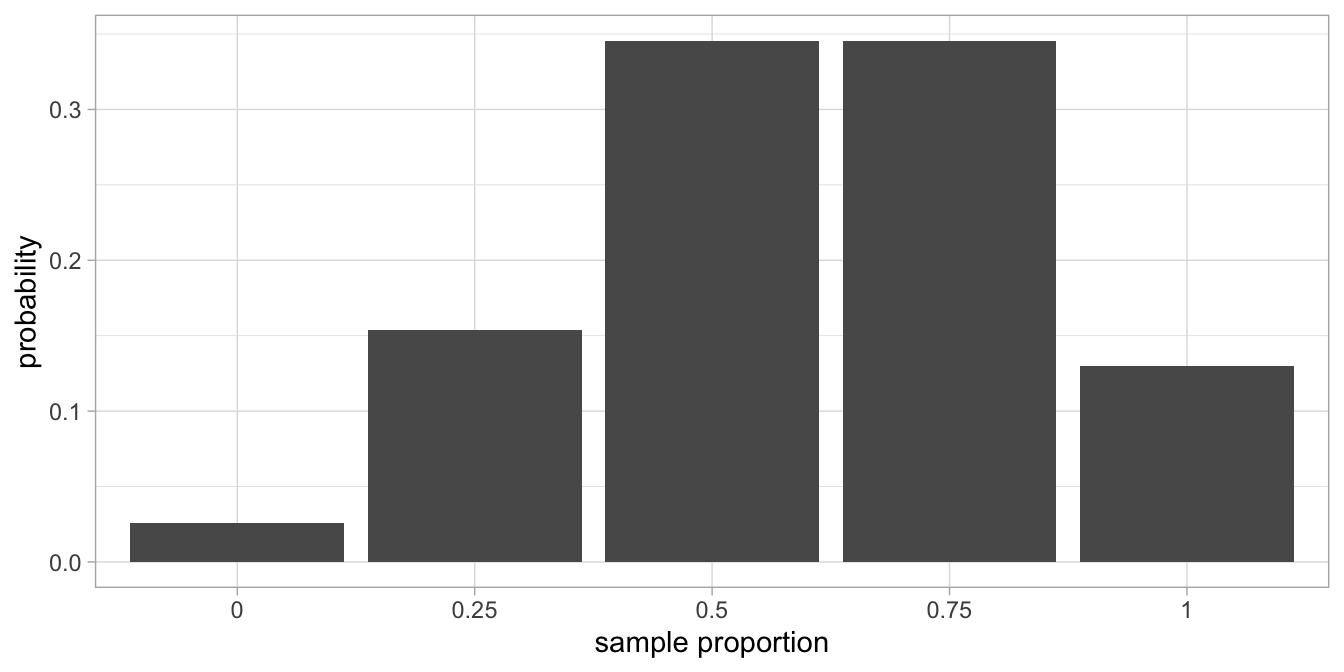
Figure 3.1: Sampling distribution of the sample proportion, when the population proportion is 0.60.
Actually, the sampling distribution that we see in Figure 3.1 is based on the binomial distribution. Using the binomial distribution, we can calculate the probabilities of getting various sample proportions in a straightforward manner, without relying on the normal distribution.
3.2 The binomial distribution (advanced)
The binomial distribution gives us the probability of obtaining a certain number of elements, given how many elements there are in total and the population probability. In our case, the binomial distribution gives us the probability of having exactly 2 elephants taller than 3.40 m, given that there are 4 elephants in our sample and the population proportion equals 0.6. Let’s go through the reasoning step by step.
The proportion of tall elephants in the population is \(p = 0.6\). The sample size equals \(n = 4\). Let’s begin with randomly picking the first elephant: what’s the probability that we select an elephant that is taller than 3.40 m? Well, that probability is equal to the proportion of 0.6. Next, what is the probability that the second elephant is taller than 3.40? Again, this is equal to 0.6.
Now something more complicated: what is the probability that both the first and the second elephant are taller than 3.40? This is equal to \(0.6 \times 0.6 = 0.36\). What is the probability that all 4 elephants are taller than 3.40 m? That is equal to \(0.6 \times 0.6 \times 0.6 \times 0.6 = 0.60^4 = 0.130\). The probability that all 4 elephants are shorter than 3.40 m is equal to \((1-0.6)^4 = 0.4^4=0.026\).
The probability for a mix of 2 tall elephants and 2 shorter elephants is more difficult to compute. You might remember from high school that it involves combinations. For example, the probability that the first 2 elephants are taller than 3.40, and the last 2 elephants shorter, is equal to \(0.6^2 \times (1-0.6)^2 = 0.058\), but there are many other ways in which we can find 2 tall elephants and 2 shorter elephants when we randomly and sequentially pick 4 elephants. There are in fact 6 different ways of randomly selecting 4 elephants where only 2 are tall. When we use A to denote a tall elephant and B to denote a short elephant, the 6 possible combinations of having two As and two Bs are in fact: AABB, BBAA, ABAB, BABA, ABBA, and BAAB.
This number of combinations is calculated using the binomial coefficient:
\[{4\choose 2} = \frac{4!}{2!2!} = 6\]
This number \({4\choose 2}\) (‘four choose two’) is called the binomial coefficient. It can be calculated using factorials: the exclamation mark \(!\) stands for factorial. For instance, \(5!\) (‘five factorial’) means \(5\times 4 \times 3 \times 2 \times 1\).
In its general form, the binomial coefficient looks like:
\[{n\choose r} = \frac{n!}{r!(n-r)!}\]
So suppose sample size \(n\) is equal to 4 and \(r\) equal to 2 (the number of tall elephants in the sample), we get:
\[{4\choose 2} = \frac{4!}{2!(n-r)!} = \frac{4!}{2!2!} = \frac{4\times 3 \times 2 \times 1}{2 \times 1 \times 2 \times 1} = 6\]
Going back to the elephant example, there are \({4\choose 2}=6\) possible ways of getting 2 tall elephants and 2 short elephants when we sequentially pick 4 elephants. Each of these possibilities has a probability of \(0.6^2 \times (1-0.6)^2 = 0.058\). This is explained in Table 3.2. For instance, the probability of getting the ordering ABAB, is equal to the multiplication of the respective probabilities: \(0.6 \times 0.4 \times 0.6 \times 0.4\). In the table you can see that the probability for any ordering is always 0.058. Since any ordering will qualify as obtaining 2 tall elephants from a total of 4, we can sum these probabilities: the probability of getting the ordering AABB or BBAA or ABAB or BABA or ABBA or BAAB, is equal to \(0.058 + 0.058 + 0.058 + 0.058 + 0.058 + 0.058 = 6 \times 0.058 = 0.348\). Here 6 is the number of combinations, calculated as the binomial coefficient \({4\choose 2}\). We could therefore in general compute the probability of having 2 tall elephants in a sample of 4 as
\[p(\#A = 2 | n = 4, p = 0.6) = {4\choose 2} \times 0.6^2 \times (1-0.6)^2 = 6 \times 0.058 = 0.348\]
| ordering | computation of probability | probability |
|---|---|---|
| AABB | 0.6 x 0.6 x 0.4 x 0.4 | 0.058 |
| ABAB | 0.6 x 0.4 x 0.6 x 0.4 | 0.058 |
| ABBA | 0.6 x 0.4 x 0.4 x 0.6 | 0.058 |
| BAAB | 0.4 x 0.6 x 0.6 x 0.4 | 0.058 |
| BABA | 0.4 x 0.6 x 0.4 x 0.6 | 0.058 |
| BBAA | 0.4 x 0.4 x 0.6 x 0.6 | 0.058 |
The probability of ending up with 2 tall elephants in a sample of 4 elephants, in any order, and where the proportion of tall elephants in the population is 0.6, is therefore equal to 0.348.
In the more general case, if you have a population with a proportion \(p\) of As, a sample size of \(n\), and you want to know the probability of finding \(r\) instances of A in your sample, it can be computed with the formula
\[p(\#A = r | n, p) = {n\choose r} \times p^r \times (1-p)^{(n-r)}\]
For example, the probability of obtaining 3 tall elephants when the total number of elephants is 4, is \({4\choose 3} \times 0.6^3 \times (1-0.6)^{1} = 4 \times 0.216 \times 0.4 = 0.346\).
When we calculate the probabilities of finding 0, 1, 2, 3, or 4 tall elephants in a sample of 4 when the population proportion is 0.6, we obtain the binomial distribution that is plotted in Figure 3.2. It is exactly the same as the sampling distribution in Figure 3.1, except that we plot the number of tall elephants in the sample on the horizontal axis, instead of the proportion. This means that we can use the binomial distribution to describe the sampling distribution of the sample proportion. To get the proportions, we simply divide the number of tall elephants in our sample by the total number of elephants (\(n\)) and we get Figure 3.1.
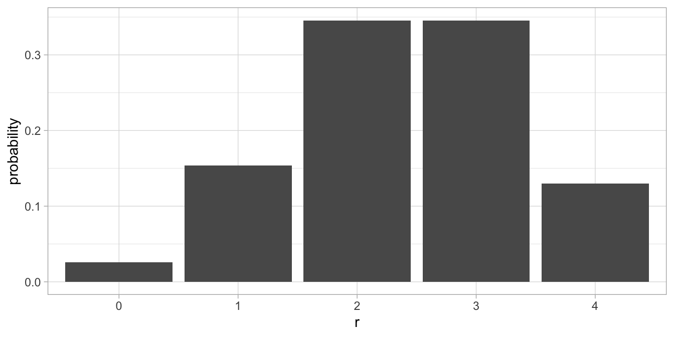
Figure 3.2: Binomial distribution with \(n=4\) and \(p=0.60\).
3.3 Confidence intervals (advanced)
Based on what we know about the binomial distribution, we can perform inference on proportions. In Chapter 2 we saw that inference is very much based on the standard error (i.e., the standard deviation of the sampling distribution). We know from theory that the variance of the binomial distribution can be easily calculated as \(n \times p \times (1-p)\). Because we want to have the variance in proportions rather than in numbers, we have to divide this variance by \(n\) to get the variance of proportions: \(\frac{n \times p \times (1-p)}{n} = p \times (1-p)\). Next, because the variance of a sampling distribution gets smaller with increasing \(n\), we divide by \(n\) again, in a similar way as we did for the sampling distribution of the sample mean in Chapter 2. Taking the square root of this variance gives us the standard deviation of the sampling distribution (i.e., the standard error):
\[\sigma_{\hat{p}} = \sqrt{\frac{p(1-p)}{n}}\]
This standard error makes it easy to construct confidence intervals. We know from the Central Limit Theorem that if \(n\) becomes infinitely large, the sampling distribution will become normal. When \(n=50\), the sampling distribution is already close to normal, as is shown in Figure 3.3. This fact, together with the standard error makes it easy to construct approximate confidence intervals.
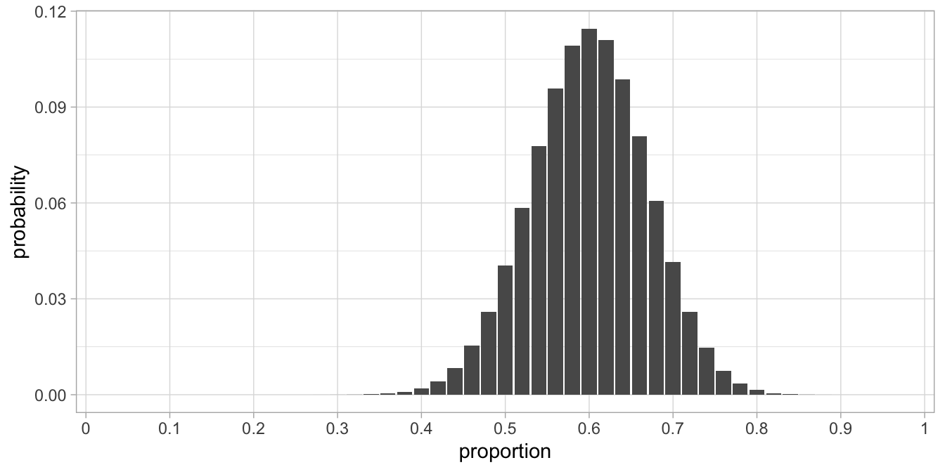
Figure 3.3: Sampling distribution with \(n=50\) and \(p=0.60\).
Suppose that we had 50 elephants in our zoo, and the manager observed that 42 of them bump their head against the doorway. That is a sample proportion of \(\frac{42}{50}= 0.84\). When we want to have a range of plausible values for the population proportion, we can construct a 95% confidence interval around this sample proportion. Because we know that for the standard normal distribution, 95% of the observations are between -1.96 and +1.96, we construct the 95% confidence interval by multiplying 1.96 with the standard error, \(\sigma_{\hat{p}} = \sqrt{\frac{p(1-p)}{n}}\).
However, since we do not know the population proportion \(p\), we have to estimate it. From theory, we know that an unbiased estimator for the population proportion is the sample proportion: \(\hat{p} = \frac{42}{50}= 0.84\). Our estimate for the standard error is then \(\sqrt{\frac{\hat{p}(1-\hat{p})}{n}} = 0.052\).
If we use that value, we get the interval from \(0.84 - 1.96 \times 0.052\) to \(0.84 + 1.96 \times 0.052\): thus, our 95% confidence interval for the population proportion runs from 0.738 to 0.942.
3.4 Null-hypothesis concerning a proportion using the Central Limit Theorem
To do statistical computations by hand using the binomial distribution is often tedious. Because of the central limit theorem, we know that for large sample sizes, the sampling distribution becomes normal. The mean of the sampling distribution is then equal to the proportion \(p\) in the population, and the standard error is equal to \(\sigma_{\hat{p}} = \sqrt{\frac{p(1-p)}{n}}\). If the sample size, \(n\), is large, we can perform null-hypothesis testing using the more familiar normal distribution.
Here we show how to do that with an example using a somewhat larger sample size of 50. Suppose that a researcher has measured all Tanzanian elephants and noted that a proportion of 0.60 was taller than 3.40 m. Suppose also that the manager in the zoo finds that 42 out of the 50 zoo elephants bump their head and are therefore taller than 3.40. How can we test the hypothesis that the zoo elephants could be a random sample of Tanzanian elephants?
To answer this question with a yes or a no, we could apply the logic of null-hypothesis testing. Let the null-hypothesis be that the population of elephants that the zoo elephants were drawn from has a proportion of 0.6 of elephants taller than 3.40 m, and the alternative hypothesis that it this proportion is not equal to 0.60.
\[\begin{aligned} H_0: p = 0.60 \\ H_A: p \neq 0.60\end{aligned}\]
Is the proportion of 0.84 that we observe in the sample (the zoo) a probable value to find if the proportion for all elephants is equal to 0.60? If this is the case, we do not reject the null-hypothesis, and believe that the zoo data could have been randomly selected from the Tanzanian population. However, if the proportion of 0.84 is very unprobable given that the population proportion is 0.60, we reject the null-hypothesis and believe that the zoo elephants were not randomly drawn from the population of Tanzanian elephants.
With null-hypothesis testing we always have to fix our \(\alpha\) first: the probability with which we are willing to accept a type I error. We feel it is really important that the sample is representative of the population, so we definitely do not want to make the mistake that we think the sample is representative (not rejecting the null-hypothesis) while it isn’t (\(H_A\) is true). This would be a type II error (check this for yourself!). If we want to minimise the probability of a type II error (\(\beta\)), we have to pick a relatively high \(\alpha\) (see Chapter 2), so let’s choose our \(\alpha = .10\).
Next, we have to choose a test statistic and determine critical values for it that go with an \(\alpha\) of .10. Because we have a relatively large sample size of 50, we assume that the sampling distribution for a proportion of 0.60 is normal. From the standard normal distribution, we know that 90% (\(1-\alpha\)!) of the values lie between \(-1.64\) and \(1.64\) (see Table 2.4). If we therefore standardise our proportion, we have a measure that should show a standard normal distribution:
\[z_p = \frac{p_s - p_0}{sd}\]
where \(z_p\) is the \(z\)-score for a proportion, \(p_s\) is the sample proportion, \(p_0\) is the population proportion assuming \(H_0\), and \(sd\) is the standard deviation of the sampling distribution, which is the standard error. Note that we should take the standard error that we get when the null-hypothesis is true. We then get
\[z_p = \frac{0.84 - 0.6}{se} = \frac{0.24}{\sqrt{\frac{p_0(1-p_0)}{n}}} = \frac{0.24}{0.069} = 3.478\]
90% of the values in any normal distribution lie between \(\pm 1.64\) standard deviations away from the mean (see Table 2.4). Here we see a \(z\)-score that exceeds these critical values, and we therefore reject the null-hypothesis. We conclude that the proportion of tall elephants observed in the sample is larger than to be expected under the assumption that the population proportion is 0.6. We decide that the zoo data are not randomly drawn from the Tanzanian population data.
The decision process is illustrated in Figure 3.4.
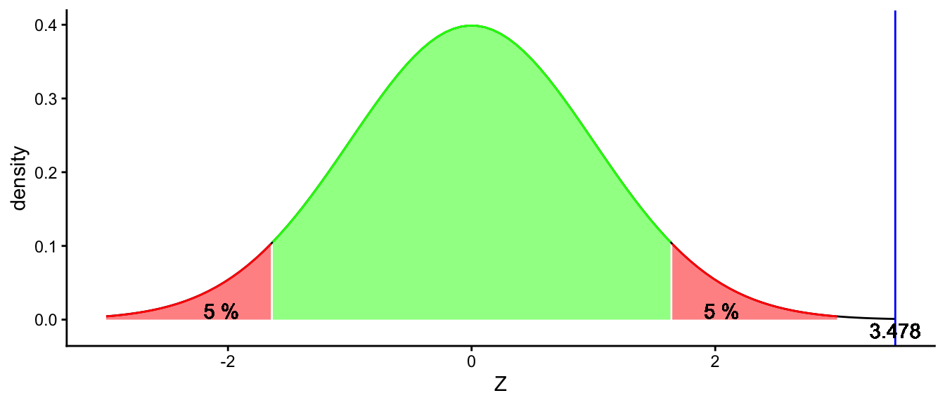
Figure 3.4: A normal distribution to test the null-hypothesis that the population proportion is 0.6. The blue line represents the z-score for our observed sample proportion of 0.84.
To get a feel for what critical z-values go together with what type I error rate, try out the interactive app in Figure 3.5. Choose a type I error rate of 10% and check that the critical z-value will be \(\pm 1.64\). Next choose a type I error rate of 5% and check that the critical z-value will become \(\pm 1.96\). Note that we apply two-tailed (two-sided) hypothesis testing here.
Figure 3.5: [Interactive] The relationship between the type I error rate \(\alpha\), and the critical \(z\)-values to reject the null-hypothesis for a proportion. Change the type I error rate, and see how that affects the critical \(z\)-value.
3.5 Inference on proportions using R
Using the normal distribution as shown in the previous section is a nice trick when you have to do the calculations by hand. However, the normal distribution is only a good approximation of the binomial distribution when you have a large sample size. Using the binomial distribution always gives you the most exact answers, but it can be very tiresome to do all the computations by hand. In this section we discuss how to let R do the calculations for you.
Suppose we have a sample of 50 elephants, and we see that 42 of them
bump their head against the doorway. What can we say about the
population: what proportion of elephants in the entire population will
bump their heads? In R, we use the binom.test() function to do
inference on proportions. This function does all the calculations using
the binomial distribution, so that the results are always trustworthy,
even for small sample sizes. We state the number of observed elephants
that bump their head (x = 42), the sample size (n = 50), the kind of
confidence interval (95%: conf.level = 0.95) and the proportion that
we want to use for the null-hypothesis (p = 0.6):
##
##  Exact binomial test
##
## data:  42 and 50
## number of successes = 42, number of trials = 50, p-value = 0.0004116
## alternative hypothesis: true probability of success is not equal to 0.6
## 95 percent confidence interval:
##  0.7088737 0.9282992
## sample estimates:
## probability of success
##                   0.84
The output shows the sample proportion: the probability of success is 0.84. This is of course \(\frac{42}{50}\). If we want to know what the most reasonable values for the population proportion are, we look at the 95% confidence interval that runs from 0.71 to 0.93. If you want to test the null-hypothesis that the population proportion is equal to 0.60, then we see that the \(p\)-value for that test is .0004. Using only three decimals, we can say the \(p\)-value is less than .001. With an \(\alpha\) of 0.10, this test is significant. We therefore conclude:
"With a binomial test, we tested the null-hypothesis that the population proportion of elephants taller than 3.40 m is equal to 0.60, with an \(\alpha\) of 0.10. Our sample proportion, based on 50 elephants, was 0.84, which is significantly different from 0.6, \(p < .001\). We therefore reject the null-hypothesis."
As said, the binomial test also works fine for small sample sizes. Let’s go back to the very first example of this chapter: the zoo manager sees that of the 4 elephants they have, 3 bump their head and are therefore taller than 3.40 m. What does that tell us about the proportion of elephants worldwide that are taller than 3.40 m? If we assume that the 4 zoo elephants were randomly selected from the entire population of elephants, we can use the binomial distribution. In this case we type in R:
##
##  Exact binomial test
##
## data:  3 and 4
## number of successes = 3, number of trials = 4, p-value = 0.625
## alternative hypothesis: true probability of success is not equal to 0.5
## 95 percent confidence interval:
##  0.1941204 0.9936905
## sample estimates:
## probability of success
##                   0.75
By default, binom.test() yields 95% confidence intervals, as can be
seen in the output.15 We see that the confidence interval for the
population proportion runs from 0.194 to 0.994. Thus, based on
this sample proportion of 0.75, we can state with some degree of
confidence that the population proportion is somewhere between 0.194 and
0.994. That’s of course not very informative, which makes sense
considering we only observe 4 elephants.
We could report:
"In our sample of 4 elephants, 3 were taller than 3.40 m. The 95% confidence interval for the proportion of elephants in the population that are taller than 3.40 m runs from 0.194 to 0.994."
or, somewhat shorter:
"Based on a sample of 4 elephants, our estimate for the proportion of elephants in the population that are taller than 3.40 m is 0.75 (95% CI: 0.194, 0.994)."
Note in the output that by default,
binom.test()chooses the null-hypothesis that the population proportion is 0.5.↩︎