Chapter 12 Linear mixed modelling: introduction
12.1 Fixed effects and random effects
In the simplest form of linear modelling, we have one dependent numeric variable, one intercept and one or more independent variables. Let’s look at a simple regression equation where dependent variable \(Y\) is predicted by an intercept \(b_0\) and a linear effect of independent variable \(X\) with regression slope parameter \(b_1\), and an error term \(e\), where we assume that the error term \(e\) comes from a normal distribution.
\[\begin{aligned} Y &= b_0 + b_1 X + e \\ e &\sim N(0, \sigma^2)\end{aligned}\]
Using this model, we know that for a person with a value of 5 for \(X\),
we expect \(Y\) to be equal to \(b_0 + b_1 \times 5\). As another example,
if \(Y\) is someone’s IQ score, \(X\) is someone’s brain size in cubic
millilitres, \(b_0\) is equal to 70, and \(b_1\) is equal to 0.1, we expect
on the basis of this model that a person with a brain size of 1500 cubic
millimetres has an IQ score of \(70 + 0.01 \times 1500\), which equals
85.
Now, for any model the predicted values usually are not the same as the
observed values. If the model predicts on the basis of my brain size
that my IQ is 140, my true IQ might be in fact 130. This discrepancy is
termed the residual: the observed \(Y\), minus the predicted \(Y\), or
\(\widehat{Y}\), so in this case the residual is
\(Y - \widehat{Y}=130-140= -10\).
Here we have the model for the relationship between IQ and brain size.
\[\begin{aligned} \texttt{IQ} &= 70 + 0.1 \times \texttt{Brain size} + e \\ e &\sim N(0, \sigma^2)\end{aligned}\]
Note that in this model, the values of 70 and 0.1 are fixed, that is, we use the same intercept and the same slope for everyone. You use these values for any person, for Henry, Jake, Liz, and Margaret. We therefore call these effects of intercept and slope fixed effects, as they are all the same for all units of analysis. In contrast, we call the \(e\) term, the random error term or the residual in the regression, a random effect. This is because the error term is different for every unit. We don’t know the specific values of these random errors or residuals for every person, but nevertheless, we assume that they come from a distribution, in this case a normal distribution with mean 0 and an unknown variance. This unknown variance is given the symbol \(\sigma^2\).
Here are a few more examples.
Suppose we study a number of schools, and for every school we use a simple linear regression equation to predict the number of students (dependent variable) on the basis of the number of teachers (independent variable). For every unit of analysis (in this case: school), the intercept and the regression slope are the same (fixed effects), but the residuals are different (random effect).
Suppose we study reaction times, and for every measure of reaction time – a trial – we use a simple linear regression equation to predict reaction time in milliseconds on the basis of the characteristics of the stimulus. Here, the unit of analysis is trial, and for every trial, the intercept and the regression slope are the same (fixed effects), but the residuals are different (random effect).
Suppose we study a number of students, and for every student we use a simple linear regression equation to predict the math test score on the basis of the number of hours of study the student puts in. Here, the unit of analysis is student, and for every student, the intercept and the regression slope are the same (fixed effects), but the residuals are different (random effect).
Let’s focus for now on the last example. What happens when we have a lot of data on students, but the students come from different schools? Suppose we want to predict average grade for every student, on the basis of the number of hours of study the student puts in. We again could use a simple linear regression equation.
\[\begin{aligned} Y &= b_0 + b_1 \texttt{hourswork} + e \\ e &\sim N(0, \sigma^2)\end{aligned}\]
That would be fine if all schools would be all very similar. But suppose that some schools have a lot of high scoring students, and some schools have a lot of low scoring students? Then school itself would also be a very important predictor, apart from the number of hours of study. One could say that the data are clustered: math test scores coming from the same school are more similar than math test scores coming from different schools. When we do not take this into account, the residuals will not show independence (see Chapter 7 on the assumptions of linear models).
One thing we could therefore do to remedy this is to include school as a
categorical predictor. We would then have to code this school variable
into a number of dummy variables. The first dummy variable called
school1 would indicate whether students are in the first school
(school1 = 1) or not (school1 = 0). The second dummy variable
\(\texttt{school2}\) would indicate whether students are in the second
school (school2 = 1) or not (school2 = 0), etcetera. You can then
add these dummy variables to the regression equation like this:
\[\begin{aligned} Y &= b_0 + b_1 \texttt{hourswork} + b_2 \texttt{school1} + b_3 \texttt{school2} + b_4 \texttt{school3} + \dots + e \nonumber\\ e &\sim N(0, \sigma^2) \nonumber\end{aligned}\]
In the output we would find a large number of effects, one for each dummy variable. For example, if the students came from 100 different schools, you would get 99 fixed effects for the 99 dummy variables. However, one could wonder whether this is very useful. As stated earlier, fixed effects are called fixed because they are the same for every unit of research, in this case every student. But working with 99 dummy variables, where students mostly score 0, this seems very much over the top. In fact, we’re not even interested in these 99 effects. We’re interested in the relationship between test score and hours of work, meanwhile taking into account that there are test score differences across schools. The dummy variables are only there to account for differences across schools; the prediction for one school is a little bit higher or lower than for another school, depending on how well students generally perform in each school.
We could therefore try an alternative model, where we treat the school effect as \(random\): we assume that every school has a different average test score, and that these averages are normally distributed. We call these average test score deviations school effects:
\[\begin{aligned} Y &= b_0 + b_1 \texttt{hourswork} + \texttt{schooleffect} + e \notag\\ \texttt{schooleffect} &\sim N(0, \sigma_s^2) \notag\\ e &\sim N(0, \sigma_e^2) \notag \end{aligned}\]
So in this equation, the intercept is fixed, that is, the intercept is the same for all observed test scores. The regression coefficient \(b_1\) for the effect of hours of work is also fixed. But the schooleffect is random, since it is different for every school. The residual \(e\) is also random, being different for every student. It could also be written like this:
\[\begin{eqnarray} Y &=& (b_0 + \texttt{schooleffect}) + b_1 \texttt{hourswork} + e \\ \texttt{schooleffect} &\sim& N(0, \sigma_s^2) \nonumber\\ e &\sim& N(0, \sigma_e^2)\nonumber \tag{12.1} \end{eqnarray}\]
This representation emphasises that for every school, the intercept is a little bit different: for school A the intercept might be \(b_0 + 2\), and for school B the intercept might be \(b_0 - 3\).
So, equation (12.1) states that every observed test score is
partly influenced by an intercept that is random, with a certain average \(b_0\) and variance \(\sigma_s^2\), that is dependent on which school students are in,
partly influenced by the number of hours of work, an effect that is the same no matter what school a student is in (fixed), and
partly influenced by unknown factors, indicated by a random residual \(e\) coming from a normal distribution with variance \(\sigma^2_e\).
To put it more formally: test score \(Y_{ij}\), that is, the test score from student \(j\) in school \(i\), is the sum of an effect of the school \(b_0 + \texttt{schooleffect}_i\) (the average test score in school \(i\)), plus an effect of hours of work, \(b_1 \times \texttt{hourswork}\), and an unknown residual \(e_{ij}\) (a specific residual for the test score for student \(j\) in school \(i\)).
\[\begin{aligned} Y_{ij} &= b_0 + \texttt{schooleffect}_i + b_1 \texttt{hourswork} + e_{ij} \\ \texttt{schooleffect}_i &\sim N(0, \sigma_s^2)\\ e_{ij} &\sim N(0, \sigma_e^2)\end{aligned}\]
So in addition to the assumption of residuals that have a normal
distribution with mean 0 and variance \(\sigma_e^2\), we also have an
assumption that the school averages have a normal distribution, in this
case with mean \(b_0\) and variance \(\sigma_s^2\).
Let’s go back to the example of reaction times. Suppose in an experiment
we measure reaction time in a large number of trials. We want to know
whether the size of the stimulus (large or small) has an effect on
reaction time. Let’s also suppose that we carry out this experiment with
20 participants, where every participant is measured during 100 trials:
50 large stimuli and 50 small stimuli, in random order. Now probably,
some participants show generally very fast responses, and some
participants show generally very slow responses. In other words, the
average reaction time for the 100 trials may vary from participant to
participant. This means that we can use participant as an important
predictor of reaction times. To take this into account we can use the
following linear equation:
\[\begin{aligned} Y_{ij} &= b_0 + \texttt{speed}_i + b_1 \texttt{size} + e_{ij} \\ \texttt{speed}_i &\sim N(0, \sigma_s^2)\\ e_{ij} &\sim N(0, \sigma_e^2)\end{aligned}\]
where \(Y_{ij}\), is the reaction time \(j\) from participant \(i\), \((b_0 + \texttt{speed}_i)\) is a random intercept representing the average speed for each participant \(i\) (where \(b_0\) is the overall average across all participants and \(\texttt{speed}_i\) the random deviation for each and every participant), \(b_1\) is the fixed effect of the size of the stimulus. Unknown residual \(e_{ij}\) is a specific residual for the reaction time for trial \(j\) of participant \(i\).
The reason for introducing random effects is that when your observed data are clustered, for instance student scores clustered within schools, or trial response times are clustered within participants, you violate the assumption of independence: two reaction times from the same person are more similar than two reaction times from different persons. Two test scores from students from the same school may be more similar than two scores from students in different schools (see Chapter 7). When this is the case, when data are clustered, it is very important to take this into account. When the assumption of independence is violated, you are making wrong inference if you use an ordinary linear model, the so-called general linear model (GLM). With clustered data, it is therefore necessary to work with an extension of the general linear model or GLM, the linear mixed model. The above models for students’ test scores across different schools and reaction times across different participants, are examples of linear mixed models. The term mixed comes from the fact that the models contain a mix of both fixed and random effects. GLMs only contain fixed effects, apart from the random residual.
If you have clustered data, you should take this clustering into account, either by using the grouping variable as a categorical predictor or by using a random factor in a linear mixed model. As a rule of thumb: if you have fewer than 10 groups, consider a fixed categorical factor; if you have 10 or more groups, consider a random factor. Two other rules you can follow are: Use a random factor if the assumption of normally distributed group differences is tenable. Use a fixed categorical factor if you are actually interested in the size of group differences.
Below, we will start with a very simple example of a linear mixed model, one that we use for a simple pre-post intervention design.
12.2 Pre-post intervention designs
Imagine a study where we hope to show that aspirin helps reduce headache. We ask 100 patients to rate the severity of their headache before they use aspirin (on a scale from 1 - 100), and to rate the severity again 3 hours after taking 500 mg of aspirin. These patients are randomly selected among people who read the NY Times and suffer from regular headaches. So here we have clustered data: we have 100 patients, and for each patient we have two scores, one before (pre) and one after (post) the intervention of taking aspirin. Of course, overall headache severity levels tend to vary from person to person, so we might have to take into account that some patients have a higher average level of pain than other patients.
The data could be represented in different ways, but suppose we have the data matrix in Table 12.1 (showing only the first five patients). What we observe in that table is that the severity seems generally lower after the intervention than before the intervention. But you may also notice that the severity of the headache also varies across patients: some have generally high scores (for instance patient 003), and some have generally low scores (for example patient 001). Therefore, the headache scores seem to be clustered, violating the assumption of independence. We can quantify this clustering by computing a correlation between the pre-intervention scores and the post-intervention scores. We can also visualise this clustering by a scatter plot, see Figure 12.1. Here it appears that there is a strong positive correlation, indicating that the higher the pain score before the intervention, the higher the pain score after the intervention.
| patient | pre | post |
|---|---|---|
| 001 | 55 | 45 |
| 002 | 63 | 50 |
| 003 | 66 | 56 |
| 004 | 50 | 37 |
| 005 | 63 | 50 |
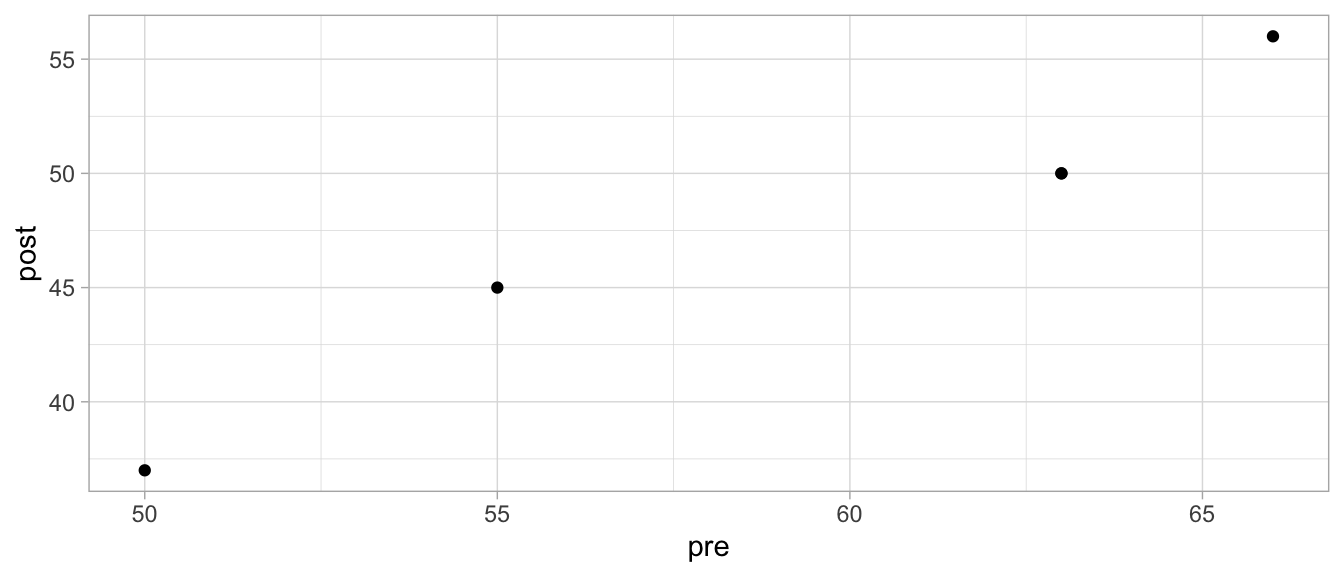
Figure 12.1: Scatterplot of pre and post headache levels.
There is an alternative way of representing the same data. Let’s look at the same data in a new format in Table 12.3. In Chapter 1 we saw that this representation is called long format.
| patient | measure | headache |
|---|---|---|
| 1 | 1 | 55 |
| 1 | 2 | 45 |
| 2 | 1 | 63 |
| 2 | 2 | 50 |
| 3 | 1 | 66 |
| 3 | 2 | 56 |
| 4 | 1 | 50 |
| 4 | 2 | 37 |
| 5 | 1 | 63 |
| 5 | 2 | 50 |
By representing the data in long format we acknowledge that there is
really only one dependent measure: headache severity. The other two
variables indicate that this variable varies across both patients and
time point (pre intervention and post intervention). There is therefore
a variable measure that indicates whether the headache severity was
measured pre intervention (measure = 1) or post intervention
(measure = 2).
Here we might consider applying a simple linear regression model, using
headache as the dependent variable and measure (1st or 2nd) as a
categorical predictor. However, since we know that there is a
correlation between the pre and post severity measures, we know that
measures also systematically vary across patients: some score high on
average and some score low on average. The assumption of independence is
therefore not tenable. Thus we have to run a linear model, including not
only an effect of measure but also an effect of patient. We then
have to decide between fixed effects or random effects for these
variables.
Let’s first look at the variable measure. Since we are really
interested in the effect of the intervention, that is, we want to know
how large the effect of aspirin is, we use a fixed effect for the time
effect (the variable measure). Moreover, the variable measure has
only two levels, which is another reason to opt for a fixed effect.
Then for the patient effect, we see that we have 100 patients. Are we
really interested by how much the average pain level in say patient 23
differs from the average pain level in say patient 45? No, not really.
We only want to acknowledge that the individual differences exist, we
want to take them into account in our model so that our inference
regarding the confidence intervals and hypothesis testing is correct. We
therefore prefer to assume random effects, assuming they are normally
distributed. We therefore end up with a fixed effect for measure and a
random effect for patient resulting in the following model:
\[\begin{aligned} Y_{ij} &= b_0 + \texttt{patient}_i + b_1 \texttt{measure2} + e_{ij} \\ \texttt{patient}_i &\sim N(0, \sigma_p^2)\\ e_{ij} &\sim N(0, \sigma_e^2)\end{aligned}\]
where \(Y_{ij}\) is the \(j\)th headache severity score (first or second)
for patient \(i\), \((b_0 + \texttt{patient}_i)\) is the average amount of
headache before aspirin that patient \(i\) deviates from the mean,
measure2 is a dummy variable, and \(b_1\) is the effect of the
intervention (by how much the severity changes from pre to post). We
assume that the average pain level for each patient shows a normal
distribution with average \(b_0\) and variance \(\sigma^2_p\). And of course
we assume that the residuals show a normal distribution.
An analysis with this model can be done with the R package lme4. That
package contains the function lmer() that works more or less the same
as the lm() function that we saw earlier, but requires the addition of
at least one random variable. Below, we run a linear mixed model, with
dependent variable headache, a regular fixed effect for the
categorical variable measure, and a random effect for the categorical
variable patient.
## Linear mixed model fit by REML ['lmerMod']
## Formula: headache ~ measure + (1 | patient)
##    Data: .
##
## REML criterion at convergence: 1189.8
##
## Scaled residuals:
##      Min       1Q   Median       3Q      Max
## -2.36239 -0.42430 -0.04973  0.49702  2.17096
##
## Random effects:
##  Groups   Name        Variance Std.Dev.
##  patient  (Intercept) 27.144   5.210
##  Residual              8.278   2.877
## Number of obs: 200, groups:  patient, 100
##
## Fixed effects:
##             Estimate Std. Error t value
## (Intercept)  59.6800     0.5952  100.28
## measure2    -10.3600     0.4069  -25.46
##
## Correlation of Fixed Effects:
##          (Intr)
## measure2 -0.342
In the output we see the results. We’re mainly focused on the fixed
effect of the intervention: does aspirin reduce headache? Where it says
‘Fixed effects:’ in the output, we see the linear model coefficients,
with an intercept of around 59 and a negative effect of the intervention
dummy variable measure2, around \(-10\). We see that the dummy variable
was coded 1 for the second measure (after taking aspirin). So, for our
dependent variable headache, we see that the expected headache
severity for the observations with a 0 for the dummy variable measure2
(that is, measure 1, which is before taking aspirin), is equal to
\(59 - (10) \times 0 = 59\).
Similarly, we see that the expected headache severity for the
observations with a 1 for the dummy variable measure2 (that is,
after taking aspirin), is equal to
\(59 - (10) \times 1 = 49 - 10 = 49\). So, expected pain severity is 10
points lower after the intervention than before the intervention.
Whether this difference is significant is indicated by a \(t\)-statistic.
We see here that the average headache severity after taking an aspirin
is significantly different from the average headache severity before
taking an aspirin, \(t = -25.46\). However, note that we do not see a
\(p\)-value. That’s because the degrees of freedom are not clear, because
we also have a random variable in the model. The determination of the
degrees of freedom in a linear mixed model is a complicated matter, with
different choices, the discussion of which is beyond the scope of this
book.
However, we do know that for whatever the degrees of freedom really are, a \(t\)-statistic of -25.46 will always be in the far tail of the \(t\)-distribution, see Appendix B. So we have good reason to conclude that we have sufficient evidence to reject the null-hypothesis that headache levels before and after aspirin intake are the same.
If we do not want to test a null-hypothesis, but want to construct a confidence interval, we run into the same problem that we do not know what \(t\)-distribution to use. Therefore we do not know with what value the standard error of 0.40 should be multiplied to compute the margin of error. We could however use a coarse rule of thump and say that the critical \(t\)-value for a 95% confidence interval is more or less equal to 2 (see Appendix B). If we do that, then we get the confidence level for the effect of aspirin: between \(-10.36 - 2 \times 0.4069 = -11.17\) and \(-10.36 + 2 \times 0.4069 = -9.55\).
Taking into account the direction of the effect and the confidence
interval for this effect, we might therefore carefully conclude that
aspirin reduces headache in the population of NY Times readers with
headache problems, where the reduction is around 10 points on a 1...100
scale (95% CI: 9.55 – 11.17).
Now let’s look at the output regarding the random effect of patient
more closely. The model assumed that the individual differences in
headache severity in the 100 patients came from a normal distribution.
How large are these individual differences actually? This can be gleaned
from the ‘Random effects:’ part of the R output. The ‘intercept’ (i.e.,
the patient effect in our model) seems to vary with a variance of 27,
which is equivalent to a standard deviation of \(\sqrt{27}\) which is
around 5.2. What does that mean exactly? Well let’s look at the equation
again and fill in the numbers:
\[\begin{aligned} Y_{ij} &= b_0 + \texttt{patient}_i + b_1 \texttt{measure2} + e_{ij} \\ Y_{ij} &= 59 + \texttt{patient}_i - 10 \texttt{measure2} + e_{ij} \\ patient_i &\sim N(0, 27)\\ e_{ij} &\sim N(0, 8)\end{aligned}\]
Since R used the the headache level before the intervention as the reference category, we conclude that the average pain level before taking aspirin is 59. However, not everybody’s pain level before taking aspirin is 59: people show variance (variation). The pain level before aspirin varies with a variance of 27, which is equivalent to a standard deviation of around 5.2. Figure 12.2 shows how much this variance actually is. It depicts a normal distribution with a mean of 59 and a standard deviation of 5.2.
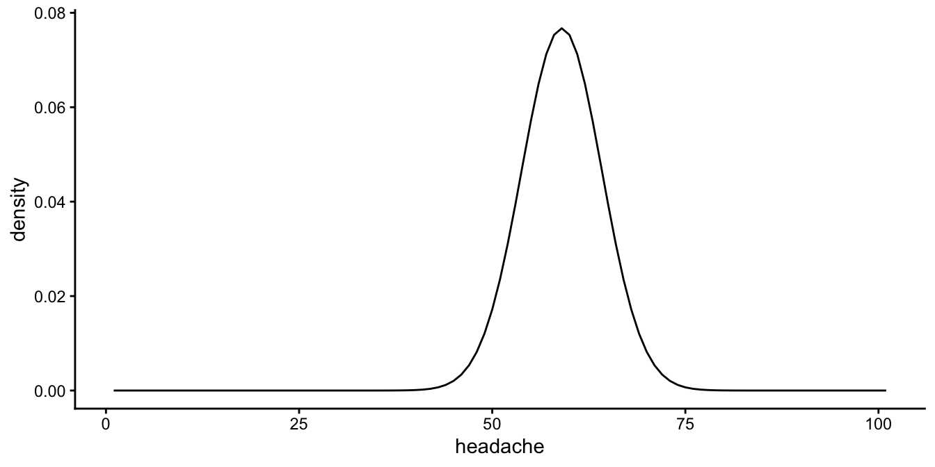
Figure 12.2: Distribution of headache scores before taking aspirin, according to the linear mixed model.
So before taking aspirin, most patients show headache levels roughly
between 50 and 70. More specifically, if we would take the middle 95% by
using plus or minus twice the standard deviation, we can estimate that
95% of the patients shows levels between \(59 - 2 \times 5.2 = 48.6\) and
\(59 + 2 \times 5.2 = 69.4\).
Now let’s look at the levels after taking aspirin. The average
headache level is equal to \(59 - 10 = 49\). So 95% of the patients shows
headache levels between \(49 - 2 \times 5.2 = 38.6\) and
\(49 + 2 \times 5.2 = 59.4\) before taking aspirin.
Together these results are visualised in Figure
12.3. In this plot you see there is
variability in headache levels before taking aspirin, and there is
variation in headache levels after taking aspirin. We also see that
these distributions have the same spread (variance): in the model we
assume that the variability in headache before aspirin is equal to the
variability after aspirin (homoscedasticity). The distributions are
equal, except for a horizontal shift: the distribution for headache
after aspirin is the same as the distribution before aspirin, except for
a shift to the left of about 10 points. This is of course the effect of
aspirin in the model, the \(b_1\) parameter in our model above.
## Warning in fortify(data, ...): Arguments in `...` must be used.
## ✖ Problematic argument:
## • show.legend = F
## ℹ Did you misspell an argument name?
## Warning in geom_label(aes(x = 70, y = 0.06), col = "blue", label = "before aspirin", : All aesthetics have length 1, but the data has 101 rows.
## ℹ Please consider using `annotate()` or provide this layer with data containing
## a single row.## Warning in geom_label(aes(x = 40, y = 0.06), col = "black", label = "3 hrs after aspirin", : All aesthetics have length 1, but the data has 101 rows.
## ℹ Please consider using `annotate()` or provide this layer with data containing
## a single row.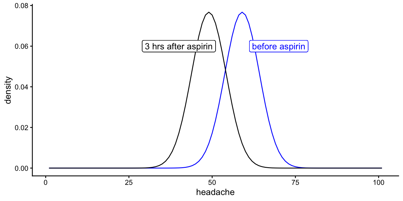
Figure 12.3: Distribution of headache scores before and after taking aspirin, according to the linear mixed model.
The fact that the two distributions before and after aspirin show the same spread (variance) was an inherent assumption in our model: we only have one random effect for patient in our output with one variance (\(\sigma^2_p\)). If the assumption of equal variance (homoscedasticity) is not tenable, then one should consider other linear mixed models. But this is beyond the scope of this book. The assumption can be checked by plotting the residuals, using different colours for residuals from before taking aspirin and for residuals from after taking aspirin.
library(modelr)
data %>%
  add_residuals(out) %>%
  add_predictions(out) %>%
  ggplot(aes(x = pred, y = resid, colour = measure)) +
  geom_point() +
  xlab("Predicted headache") +
  ylab("Residual") +
  scale_colour_brewer(palette = "Set1") + # use nice colours
  theme_light()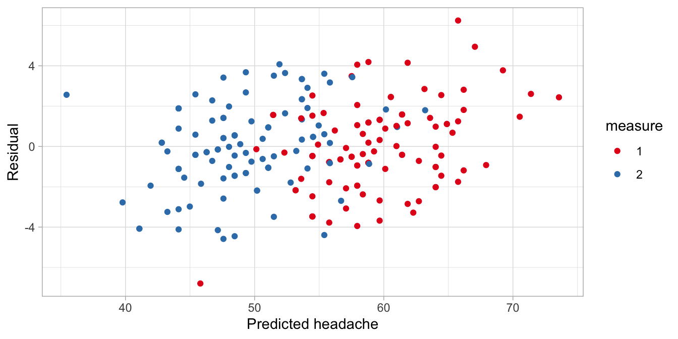
Alternatively one could create a box plot.
data %>%
  add_residuals(out) %>%
  ggplot(aes(x = measure, y = resid)) +
  geom_boxplot() +
  xlab("Measure") +
  ylab("Residual") +
  theme_light()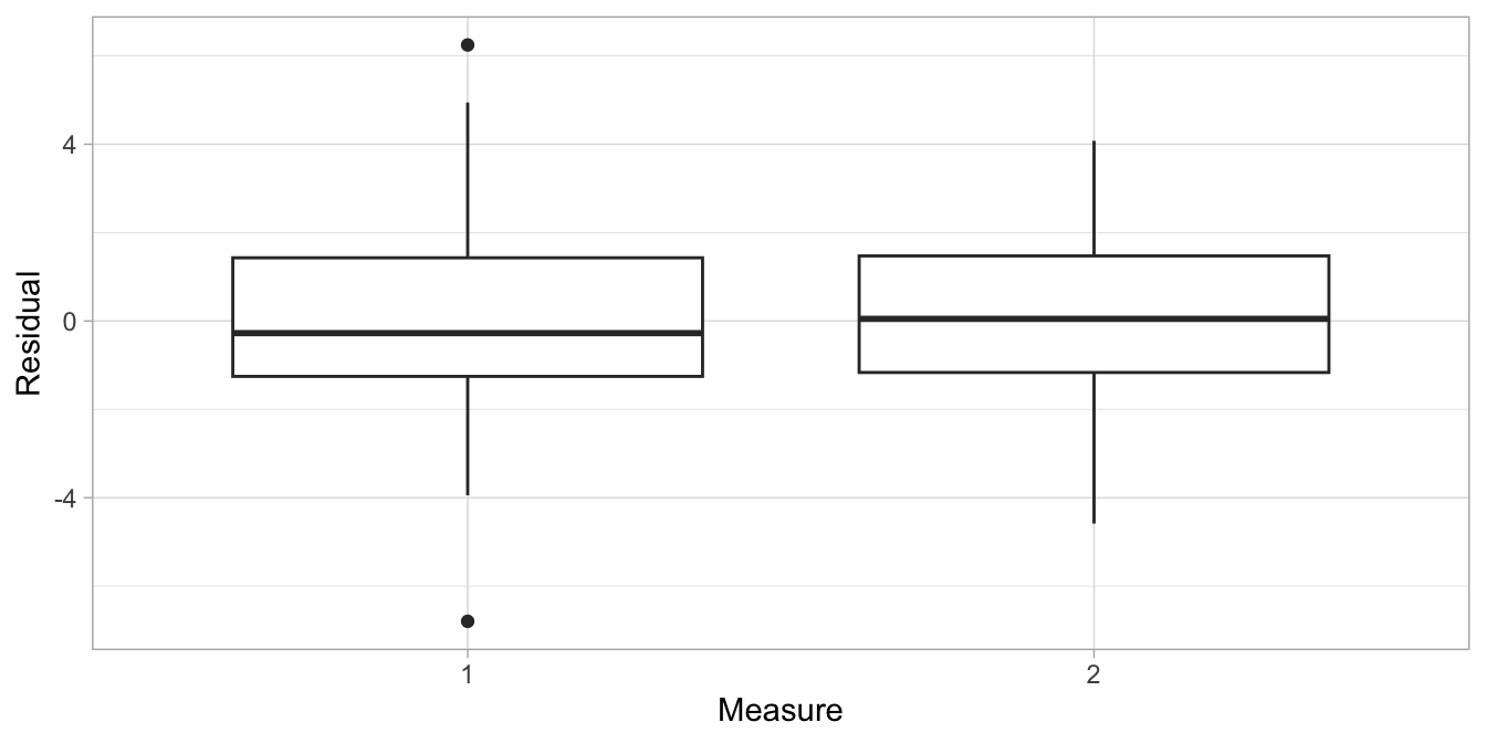
The plots show that the variation in the residuals is about the same for pre and post aspirin headache levels (box plot) and for all predicted headache levels (scatter plot). This satisfies the assumption of homogeneity of variance.
If all assumptions are satisfied, you are at liberty to make inferences
regarding the model parameters. We saw that the effect of aspirin was
estimated at about 10 points with a rough 95% confidence interval, that
was based on the rule of thumb of 2 standard errors around the estimate.
For people that are uncomfortable with such quick and dirty estimates,
it is also possible to use Satterthwaite’s approximation of the degrees
of freedom. You can obtain these, once you load the package lmerTest.
After loading, your lmer() analysis will yield (estimated) degrees of
freedom and the \(p\)-values associated with the \(t\)-statistics and those
degrees of freedom.
## Linear mixed model fit by REML. t-tests use Satterthwaite's method [
## lmerModLmerTest]
## Formula: headache ~ measure + (1 | patient)
##    Data: .
##
## REML criterion at convergence: 1189.8
##
## Scaled residuals:
##      Min       1Q   Median       3Q      Max
## -2.36239 -0.42430 -0.04973  0.49702  2.17096
##
## Random effects:
##  Groups   Name        Variance Std.Dev.
##  patient  (Intercept) 27.144   5.210
##  Residual              8.278   2.877
## Number of obs: 200, groups:  patient, 100
##
## Fixed effects:
##             Estimate Std. Error       df t value Pr(>|t|)
## (Intercept)  59.6800     0.5952 124.7464  100.28   <2e-16 ***
## measure2    -10.3600     0.4069  99.0000  -25.46   <2e-16 ***
## ---
## Signif. codes:  0 '***' 0.001 '**' 0.01 '*' 0.05 '.' 0.1 ' ' 1
##
## Correlation of Fixed Effects:
##          (Intr)
## measure2 -0.342
The degrees of freedom for effect of measure2 is 99. If we look in
Appendix B or check
using R, we see that the critical \(t\)-value with 99 degrees of freedom
for a 95% confidence interval is equal to 1.98. That’s very close to our
rough estimate of 2.
## [1] 1.984217If we calculate the 95% confidence interval using the new critical value, we obtain \(-10.36 - 1.98 \times 0.41 = -11.17\) and \(-10.36 + 1.98 \times 0.41 = -9.55\). That’s only a minor difference with what we saw before.
12.3 Reporting on a linear mixed model for pre-post data
When you want to write down the results from a linear mixed model, it is important to explain what the model looked like, in terms of fixed and random effects. Usually it is not necessary to mention what method you used to determine degrees of freedom (e.g., Satterthwaite’s method).
If you would have to report on the aspirin study illustrated above, you could write down the results as follows:
"In order to estimate the effect of aspirin, headache measures were collected in 100 patients: one measure before aspirin intake and one measure after aspirin intake. The data were analysed using a linear mixed model, with a fixed effect for measure (before/after) and a random effect for patient. The results showed that the average headache score was 10.36 (SE = 0.41) points lower after aspirin intake than before intake."
If you want to include a confidence interval, you can compute it as shown above using the degrees of freedom reported by the lmerTest package. We saw that the 95% confidence interval runs from \(-10.36 - 1.98 \times 0.41\) to \(-10.36 + 1.98 \times 0.41\), that is, from -11.17 to -9.55. The value of -10.36 is negative, meaning that the scores were lower after aspirin. You can report this negative number, but it sounds strange to state that scores were on average -10.36 higher after aspirin intake. Makes more sense to switch the signs and state that the scores were on average 10.36 lower.
We therefore can report:
"The results showed that the average headache score was 10.36 (SE = 0.41, 95% CI: 9.55, 11.17) points lower after aspirin intake than before intake."
If the objective of the study was to test the null-hypothesis that the effect of aspirin equals 0, then you could report:
"In order to test the null-hypothesis that the effect of aspirin on headache equals 0, headache measures were collected in 100 patients: one measure before aspirin intake and one measure after aspirin intake. The data were analysed using a linear mixed model, with a fixed effect for measure (before/after) and a random effect for patient. The results showed that the null-hypothesis could be rejected, \(t(99) = -25.46, p < .001\). Headache level after aspirin intake (\(M = 49.32\)) was significantly lower than headache level before aspirin intake (\(M = 59.68\))."
Usually no mention is made of the variance of the random effects, if it is not relevant to the research question.