Chapter 5 Inference for linear models

In Chapter 4 on regression we saw how a linear equation can describe a data set: the linear equation describes the behaviour of one variable, the dependent variable, on the basis of one or more other variables, the independent variable(s). Sometimes we are indeed interested in the relationship between two variables in one given data set. For instance, a primary school teacher wants to know how well the exam grades in her class of last year predict how well the same students do on another exam a year later.

But very often, researchers are not interested in the relationships between variables in one data set on one specific group of people, but interested in the relationship between variables in general, not limited to only the observed data. For example, a researcher would like to know what the relationship is between the temperature in a brewery and the amount of beer that goes into the beer bottles. In order to study the effect of temperature on volume, the researcher measures the volume of beer in a limited collection of 200 bottles under standard conditions of 20 degrees Celsius and determines from log files the temperature in the factory during production for each measured bottle. The linear equation might be $\texttt{volume} = 32.35 -0.1207 \times \texttt{temp} + e$, see Figure 5.1. Thus, for every unit increase in degrees Celsius, say from 20 to 21 degrees, the volume of beer that is measured increases by -0.1207 centilitres, or put differently, the volume of beer decreases by 0.1207.

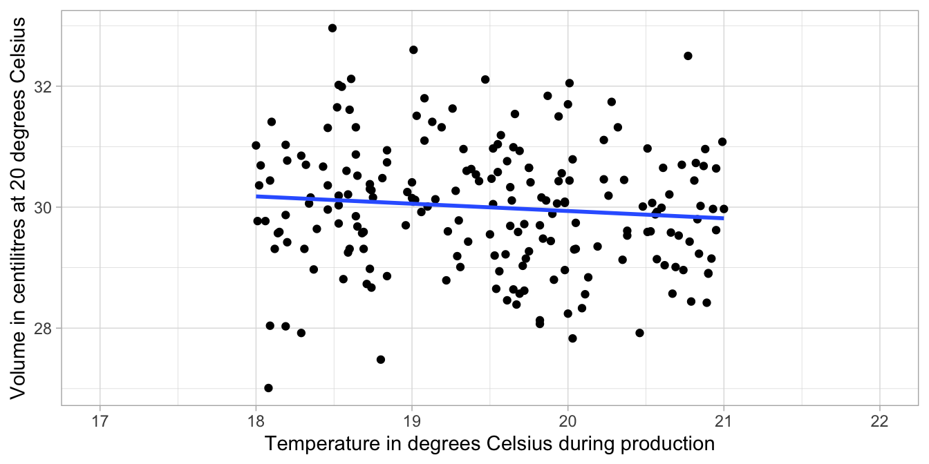
Figure 5.1: The relationship between temperature and volume in a sample of 200 bottles.

But the researcher is not at all interested in these 200 bottles specifically: the question is what would the linear equation be if the researcher had used information about all bottles produced in the same factory? In other words, we may know about the linear relationship between temperature and volume in a sample of bottles, but we might really be interested to know what the relationship would look like had we been able to measure the volume in all bottles.

In this chapter we will see how to do inference in the case of a linear model. Many important concepts that we already saw in earlier chapters will be mentioned again. Some repetition of those rather difficult concepts will be helpful, especially when now discussed within the context of linear models.

5.1 Population data and sample data

In the beer bottle example above, the volume of beer was measured in a total of 200 bottles. Let’s do a thought experiment, similar to the one in Chapter 2. Suppose we could have access to volume data about all bottles of beer on all days on which the factory was operating, including information about the temperature for each day of production. Suppose that the total number of bottles produced is 80,000 bottles. When we plot the volume of each bottle against the temperature of the factory we get the scatter plot in Figure 5.2.

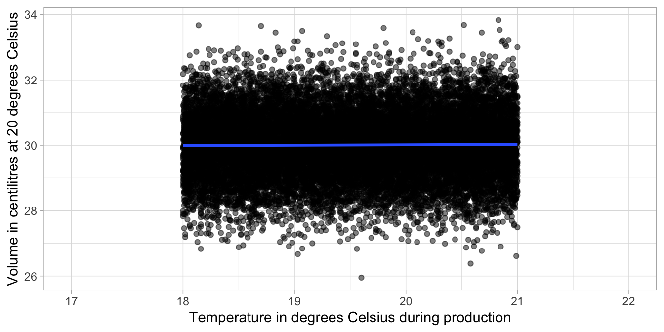
Figure 5.2: The relationship between temperature and volume in all 80,000 bottles.

In our thought experiment, we could determine the regression equation using all bottles that were produced: all 80,000 of them. We then find the blue regression line displayed in Figure 5.2. Its equation is $\texttt{volume} = 29.98 + 0.001 \times \texttt{temp} + e$. Thus, for every unit increase in temperature, the volume increases by 0.001 centilitres. Thus, the slope is slightly positive in the population, but negative in the sample of 200 bottles.

In the data example above, data were only collected on 200 bottles. These bottles were randomly selected¹⁸: there were many more bottles but we could measure only a limited number of them. This explains why the regression equation based on the sample differed from the regression equation based on all bottles: we only see part of the data.

Here we see a discrepancy between the regression equation based on the sample, and the regression equation based on the population. We have a slope of 0.001 in the population, and we have a slope of -0.1207 in the sample. Also the intercepts differ. To distinguish between the coefficients of the population and coefficients of the sample, a population coefficient is often denoted by the Greek letter $\beta$ and a sample coefficient by the Roman letter $b$.

\[\begin{aligned} Population: \texttt{volume} &= \beta_0 + \beta_1 \times \texttt{temp} = 29.98 + 0.001 \times \texttt{temp} \nonumber\\ Sample: \texttt{volume} &= b_0 + b_1 \times \texttt{temp} = 32.35 -0.1207 \times \texttt{temp} \nonumber\end{aligned}\]

The discrepancy between the two equations is simply the result of chance: had we selected another sample of 200 bottles, we probably would have found a different sample equation with a different slope and a different intercept. The intercept and slope based on sample data are the result of chance and therefore different from sample to sample. The population intercept and slope (the true ones) are fixed, but unknown. If we want to know something about the population intercept and slope, we only have the sample equation to go on. Our best guess for the population equation is the sample equation: the unbiased estimator for a regression coefficient in the population is the sample coefficient. But how certain can we be about how close the sample intercept and slope are to the population intercept and slope?

5.2 Random sampling and the standard error

In order to know how close the intercept and slope in a sample are to their values in the population, we do another thought experiment. Let’s see what happens if we take more than one random sample of 200 bottles.

We put the 200 bottles that we selected earlier back into the population and we again blindly pick a new collection of 200 bottles. We then measure for each bottle the volume of beer it contains and we determine the temperature in the factory on the day of its production. We then apply a regression analysis and determine the intercept and the slope. Next, we put these bottles back into the population, draw a second random sample of 200 bottles and calculate the intercept and slope again.

You can probably imagine that if we repeat this procedure of randomly picking 200 bottles from a large population of 80,000, each time we find a different intercept and a different slope. Let’s carry out this procedure 100 times by a computer. Table 5.1 shows the first 10 regression equations, each based on a random sample of 200 bottles. If we then plot the histograms of all 100 sample intercepts and sample slopes we get Figure 5.3. Remember from Chapters 2 and 3 that these are called sampling distributions. Here we look at the sampling distributions of the intercept and the slope.

Table 5.1: Ten different sample equations based on ten different random samples from the population of bottles.
sample	equation
1	volume = 28.87 + 0.06 x temperature + e
2	volume = 30.84 – 0.05 x temperature + e
3	volume = 31.05 – 0.06 x temperature + e
4	volume = 31.67 – 0.09 x temperature + e
5	volume = 30.59 – 0.03 x temperature + e
6	volume = 29.53 + 0.02 x temperature + e
7	volume = 28.36 + 0.08 x temperature + e
8	volume = 27.78 + 0.11 x temperature + e
9	volume = 28.29 + 0.09 x temperature + e
10	volume = 30.75 – 0.03 x temperature + e

The sampling distributions in Figure 5.3 show a large variation in the intercepts, and a smaller variation in the slopes (i.e., all values very close to another).

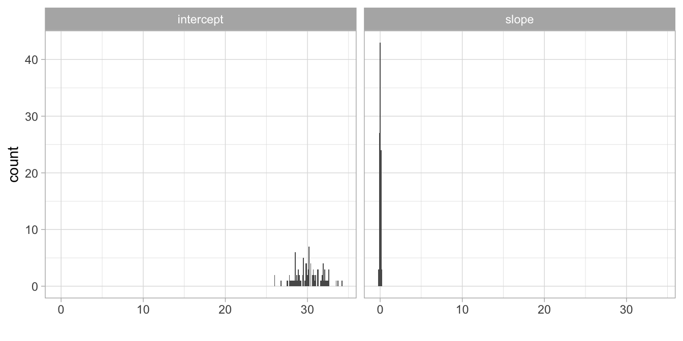
Figure 5.3: Distribution of the 100 sample intercepts and 100 sample slope.

For now, let’s focus on the slope. We do that because we are mostly interested in the linear relationship between volume and temperature. However, everything that follows also applies to the intercept. In Figure 5.4 we see the histogram of the slopes if we carry out the random sampling 1000 times. We see that on average, the sample slope is around $0.001$, which is the population slope (the slope if we analyse all bottles). But there is variation around that mean of $0.001$: the standard deviation of all 1000 sample slopes turns out to be 0.08.

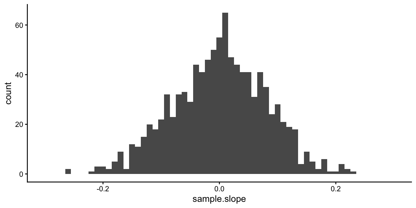
Figure 5.4: Distribution of 1000 sample slopes.

Remember from Chapter 2 that the standard deviation of the sampling distribution is called the standard error. The standard error for the sampling distribution of the sample slope represents the uncertainty about the population slope. If the standard error is large, it means that if we would draw many different random samples from the same population data, we would get very different sample slopes. If the standard error is small, it means that if we would draw many different random samples from the same population data, we would get sample slopes that are very close to one another, and very close to the population slope.¹⁹

5.2.1 Standard error and sample size

Similar to the sample mean, the standard error for a sample slope depends on the sample size: how many bottles there are in each random sample. The larger the sample size, the smaller the standard error, the more certain we are about the population slope. In the above example, the sample size is 200 bottles.

The left panel of Figure 5.5 shows the distribution of the sample slope where the sample size is 2. You see that for quite a number of samples, the slope is larger than 10, even if the population slope is 0.001. But when you increase the number of bottles per sample to 20 (in the right panel), you are less dependent on chance observations. With large sample sizes, your results from a regression analysis become less dependent on chance, become more stable, and therefore more reliable.

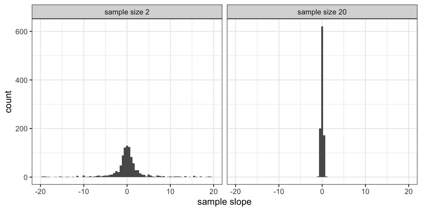
Figure 5.5: Distribution of the sample slope when sample size is 2 (left panel) and when sample size is 20 (right panel).

In Figure 5.5 we see the sampling distributions of the sample slope where the sample size is either 2 (left panel) or 20 (right panel). We see quite a lot of variation in sample slopes with sample size equal to 2, and considerably less variation in sample slopes if sample size is 20. This shows that the larger the sample size, the smaller the standard error, the larger the certainty about the population slope. The dependence of a sample slope on chance and sample size is also illustrated in Figure 5.6.

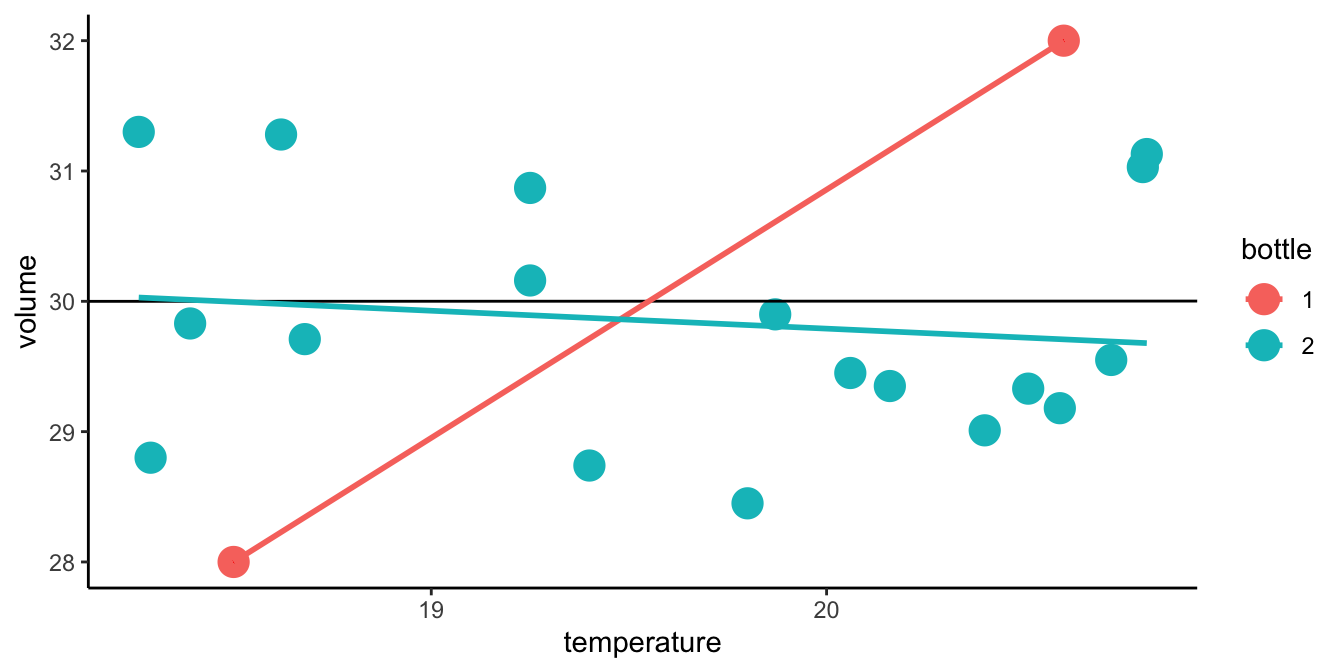
The averaging effect of increasing sample size. The scatter plot shows the relationship between temperature and volume for a random sample of 20 bottles (the dots); the first two bottles in the sample are marked in red. The red line would be the sample slope based on these first two bottles, the blue line is the sample slope based on all 20 bottles, and the black line represents the population slope, based on all 80,000 bottles. This illustrates that the larger the sample size, the closer the sample regression line is expected to be to the population regression line.

Figure 5.6: The averaging effect of increasing sample size. The scatter plot shows the relationship between temperature and volume for a random sample of 20 bottles (the dots); the first two bottles in the sample are marked in red. The red line would be the sample slope based on these first two bottles, the blue line is the sample slope based on all 20 bottles, and the black line represents the population slope, based on all 80,000 bottles. This illustrates that the larger the sample size, the closer the sample regression line is expected to be to the population regression line.

5.2.2 From sample slope to population slope

In the previous section we saw that if we have a small standard error, we can be relatively certain that our sample slope is close to the population slope. We did a thought experiment where we knew everything about the population intercept and slope, and we drew many samples from this population. In reality, we don’t know anything about the population: we only have one sample of data. So suppose we draw a sample of 200 bottles from an unknown population of bottles, and we find a slope of 1, we have to look at the standard error to know how close that sample slope is to the population slope.

For example, suppose we find a sample slope of 1 and the standard error is equal to 0.1. Then we know that the population slope is more likely to be in the neighbourhood of values like 0.9, 1.0, or 1.1 than in the neighbourhood of 10 or -10 (we know that when using the empirical rule, see Chap. 1).

Now suppose we find a sample slope of 1 and the standard error is equal to 10. Then we know that the sample slope is more likely to be somewhere in the neighbourhood of values like -9, 1 or 11, than around values in the neighbourhood of -100 or +100. However, values like -9, 1 and 11 are quite far apart, so actually we have no idea what the population slope is; we don’t even know whether the population slope is positive or negative! The standard error is simply too large.

As we have seen, the standard error depends very much on sample size. Apart from sample size, the standard error for a slope also depends on the variance of the independent variable, the variance of the dependent variable, and the correlations between the independent variable and other independent variables in the equation. We will not bore you with the complicated formula for the standard error for regression coefficients in the case of multiple regression²⁰. But here is the formula for the standard error for the slope coefficient if you have only one predictor variable $X$:

\[\begin{equation} \begin{split} \sigma_{\widehat{b_1}} &= \sqrt{ \frac{ s^2_R} {s^2_X \times (n-1)}} \notag\\ &= \sqrt{ \frac{ \frac{\sum_i ( Y_i - \widehat{Y_i} )^2}{n - 2} } {\frac{\sum_i ( X_i - \bar{X} )^2} {n-1} \times (n-1) }} \end{split} \tag{5.1} \end{equation}\]

where $b_1$ is the slope coefficient in the sample, $n$ is sample size, $s^2_R$ is the sample variance of the residuals, and $s^2_X$ the sample variance of independent variable $X$. From the formula, you can see that the standard error $\sigma_{\widehat{b_1}}$ becomes smaller when sample size $n$ becomes larger.

It’s not very useful to memorise this formula; you’d better let R do the calculations for you. But an interesting part of the formula is the nominator: $\frac{SSR}{n-2}$. This is the sum of the squared residuals, divided by $n-2$. Remember from Chapter 1 that the definition of the variance is the sum of squares divided by the number of values. Thus it looks like we are looking at the variance of the residuals. Remember from Chapter 2 that when we want to estimate a population variance, a biased estimator is the variance in the sample. In order to get an unbiased estimate of the variance, we have to divide by $n-1$ instead of $n$. This was because when computing the sum of squares, we assume we know the mean. Here we are computing the variance of the residuals, but it’s actually an unbiased estimator of the variance in the population, because we divide by $n-2$: when we compute the residuals, we assume we know the intercept and the slope. We assume two parameters, so we divide by $n-2$. Thus, when we have a linear model with 2 parameters (intercept and slope), we have to divide the sum of squared residuals by $n-2$ in order to obtain an unbiased estimator of the variance of the residuals in the population.

From the equation, we see that the standard error becomes larger when there is a large variation in the residuals, it becomes smaller when there is a large variation in predictor variable $X$, and it becomes smaller with large sample size $n$.

5.3 $t$-distribution for the model coefficients

When we look at the sample distribution of the sample slope, for instance in Figure 5.4, we notice that the distribution looks very much like a normal distribution. From the Central Limit Theorem, we know that the sampling distribution will become very close to normal for large sample sizes. Using this sampling distribution for the slope we could compute confidence intervals and do null-hypothesis testing, similar to what we did in Chapters 2 and 3.

For large sample sizes, we could assume the normal distribution, and when we standardise the slope coefficient, we can look up in tables such as in Appendix A the critical value for a particular confidence interval. For instance, 200 bottles is a large sample size. When we standardise the sample slope – let’s assume we find a slope of 0.05 –, we need to use the values -1.96 and +1.96 to obtain a 95% confidence interval around 0.05. The margin of error (MoE) is then 1.96 times the standard error. Suppose that the standard error is 0.10. The MoE is then equal to $1.96 \times 0.10 = 0.196$. The 95% interval then runs from $0.05 - 0.196 = -0.146$ to $0.05 + 0.196 = 0.246$.

However, this approach does not work for small sample sizes. Again this can be seen when we standardise the sampling distribution. When we standardise the slope for each sample, we subtract the sample slope from the population slope $\beta_1$, and have to divide each time by the standard error (the standard deviation). But when we do that

\[\begin{equation} t = \frac {b_1 - \beta_1} {\widehat{\sigma_{\widehat{b_1}}}} = \frac {b_1 - \beta_1} {\sqrt{ \frac{ s^2_R} {s^2_X \times (n-1)}}} \tag{5.2} \end{equation}\]

we immediately see the problem that when we only have sample data, we have to estimate the standard error. In each sample, we get a slightly different estimated standard error, because each time, the variation in the residuals ($s^2_R$) is a little bit different, and also the variation in the predictor variable ($s^2_X$). If sample size is large, this is not so bad: we then can get very good estimates of the standard error so there is little variation across samples. But when sample size is small, both $s^2_R$ and $s^2_X$ are different from sample to sample (due to chance), and the estimate of the standard error will therefore also vary a lot. The result is that the distribution of the standardised $t$-value from Equation (5.2) will only be close to normal for large sample size, but will have a $t$-distribution in general.

Because the standard error is based on the variance of the residuals, and because the variance of the residuals can only be computed if you assume a certain intercept and a certain slope, the degrees of freedom will be $n-2$.

Let’s go back to the example of the beer bottles. In our first random sample of 200 bottles, we found a sample slope of -0.121. We also happened to know the population slope, which was 0.001. From our computer experiment, we saw that the standard deviation of the sample slopes with sample size 200 was equal to 0.08. Thus, if we fill in the formula for the standardised slope $t$, we get for this particular sample

\[t = \frac{-0.1207-0.001}{0.08}= -1.52\]

In this section, when discussing $t$-statistics, we assumed we knew the population slope $\beta$, that is, the slope of the linear equation based on all 80,000 bottles. In reality, we never know the population slope: the whole reason to look at the sample slope is to have an idea about the population slope. Let’s look at the confidence interval for slopes.

5.4 Confidence intervals for the slope

Since we don’t know the actual value of the population slope $\beta_1$, we could ask the personnel in the beer factory what they think is a likely value for the slope. Suppose Mark says he believes that a slope of 0.1 could be true. Well, let’s find out whether that is a reasonable guess, given that the sample slope is -0.121. Now we assume that the population slope $\beta_1$ is 0.1, and we compute the $t$-statistic for our sample slope -0.121:

\[t = \frac{-0.121-0.1}{0.08}= -2.7\]

Thus, we compute how many standard errors the sample value is away from the hypothesised population value 0.1. If the population value is indeed 0.1, how likely is it that we find a sample slope of -0.121?

From the $t$-distribution, we know that such a $t$-value is very unlikely: the probability of finding a sample slope -2.7 standard deviations or more away from a population slope of 0.1 is less than 0.0075341. How do we know that? Well, the $t$-statistic is -2.7 and the degrees of freedom is $200-2=198$. The cumulative proportion of a $t$-value can be looked up in R:

pt(-2.7, df = 198)

## [1] 0.003767051

That means that a proportion of 0.0037671 of all values in the $t$-distribution with 198 degrees of freedom are lower than -2.7. Because the $t$-distribution is symmetric, we then also know that 0.0037671 of all values are larger than 2.7. If we add up these two numbers, we know that 0.0075341 of all values in a $t$-distribution are less than -2.7 or more than 2.7. That means that if the population slope is 0.1, we only find a sample slope of $\pm -0.121$ or more extreme with a probability of 0.0075341. That’s very unlikely.

Because we know that such a $t$-value of $\pm 2.7$ or more extreme is unlikely, we know that a sample slope of -0.1206874 is unlikely if the population slope is equal to 0.1. Therefore, we feel 0.1 is not a realistic value for the population slope.

Now let’s ask Martha. She thinks a reasonable value for the population slope is 0, as she doesn’t believe there is a linear relationship between temperature and volume. She suspects that the fact that we found a sample slope that was not 0 was a pure coincidence. Based on that hypothesis, we compute $t$ again and find:

\[t = \frac{-0.121-0}{0.08}= -1.5\]

In other words, if we believe Martha, our sample slope is only about 1.5 standard deviation away from her hypothesised value. That’s not a very bad idea, since from the $t$-distribution we know that the probability of finding a value more than 1.5 standard deviations away from the mean (above or below) is $13.35$%. You can see that by asking R:

pt(-1.5, df = 198) * 2

## [1] 0.1352072

Thirteen percent, that’s about 1 in 7 or 8 times. That’s not so improbable. In other words, if the population slope is truly 0, then our sample slope of $-0.121$ is quite a reasonable finding. If we reverse this line of reasoning: if our sample slope is $-0.121$, with a standard error of $0.08$, then a population slope of 0 is quite a reasonable guess! It is reasonable, since the difference between the sample slope and the hypothesised value is only $1.5$ standard errors.

So when do we no longer feel that a person’s guess of the population slope is reasonable? Perhaps if the probability of finding a sample slope of at least a certain size given a hypothesised population slope is so small that we no longer believe that the hypothesised value is reasonable. We might for example choose a small probability like 1%. We know from the $t$-distribution with 198 degrees of freedom that 1% of the values lie at least $2.6$ standard deviations above and below the mean.

qt(0.005, df = 198)

## [1] -2.600887

This is shown in Figure 5.7. So if our sample slope is more than $2.6$ standard errors away from the hypothesised population slope, then that population slope is not a reasonable guess. In other words, if the distance between the sample slope and the hypothesised population slope is more than 2.6 standard errors, then the hypothesised population slope is no longer reasonable.

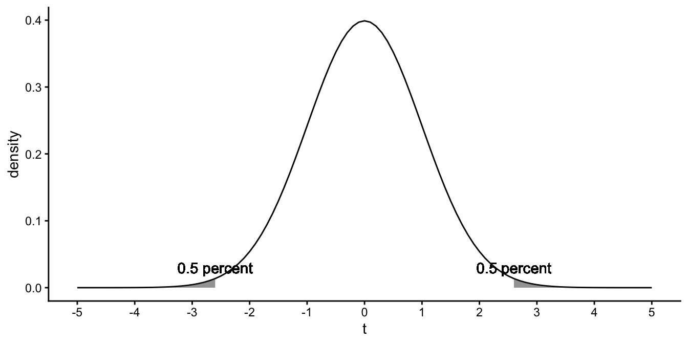
Figure 5.7: The $t$-distribution with 198 degrees of freedom.

This implies that any value closer than $2.6$ standard errors from the sample slope is a collection of reasonable values for the population slope.

Thus, in our example of the 200 bottles with a sample slope of $-0.121$ and a standard error of $0.08$, the interval from $-0.121- 2.6 \times 0.08$ to $-0.121+ 2.6 \times 0.08$ contains reasonable values for the population slope. If we do the calculations, we get the interval from $-0.33$ to $0.09$. If we would have to guess the value for the population slope, our guess would be that it would lie somewhere between between -0.33 and 0.09, if we feel that 1% is a small enough probability.

In data analysis, such an interval that contains reasonable values for the population value, if we only know the sample value, is called a confidence interval, as we know from Chapter 2. Here we’ve chosen to use $2.6$ standard errors as our cut-off point, because we felt that 1% would be a small enough probability to dismiss the real population value as a reasonable candidate (type I error rate). Such a confidence interval based on this 1% cut-off point is called a 99% confidence interval.

Particularly in social and behavioural sciences, one also sees 95% confidence intervals. The critical $t$-value for a type I error rate of 0.05 and 198 degrees of freedom is 1.97.

qt(0.975, df = 198)

## [1] 1.972017

Thus, 5% of the observations lie more than 1.97 standard deviations away from the mean, so that the 95% confidence interval is constructed by subtracting/adding 1.97 standard errors from/to the sample slope. Thus, in the case of our bottle sample, the 95% confidence interval for the population slope is from $-0.121- 1.97 \times 0.08$ to $-0.121+ 1.97 \times 0.08$, so reasonable values for the population slope are those values between $-0.28$ and $0.04$.

We could report about this in the following way, mentioning sample size, the sample slope, the standard error, and the confidence interval.

"Based on 200 randomly sampled bottles, we found a slope of -0.121 (SE = $0.08$, 95% CI: -0.28, 0.04)."

Luckily, this interval contains the true value; we happen to know that the population slope is equal to 0.001. In real life, we don’t know the population slope and of course it might happen that the true population value is not in the 95% confidence interval. If you want to make the likelihood of this being the case smaller, then you can use a 99%, a 99.9% or an even larger confidence interval.

5.5 Residual degrees of freedom in linear models

What does the term, "degrees of freedom" mean? In Chapter 2 we discussed degrees of freedom in the context of doing inference about a population mean. We saw that degrees of freedom referred to the number of values in the final calculation of a statistic that are free to vary. More specifically, the degrees of freedom for a statistic like $t$ are equal to the number of independent scores that go into the estimate, minus the number of parameters used as intermediate steps in the estimation of the parameter itself. There, we computed a $t$-statistic for the sample mean. Because in the computation of the $t$-statistic for a sample mean, we divide by the standard error for the mean, and that this in turn requires assuming a certain value for the mean, we had $n-1$ degrees of freedom.

Here, we are talking about $t$-statistics for linear models. In the case of a simple regression model, we only have one intercept and one slope. In order to compute a $t$-value, for the slope for example, we have to estimate the standard error as well. In Equation (5.1) we see that in order to estimate the standard error, we need to compute the residuals $e_i = Y_i-\hat{Y_i}$. But you can only compute residuals if you have predictions for the dependent variable, $\hat{Y_i}$, and for that you need an intercept and a slope coefficient. Thus, we need to assume we know two parameters, in order to calculate a $t$-value. With sample means we only assumed we knew the mean, and therefore had $n-1$ degrees of freedom. In case of a linear model where we assume one intercept and one slope, we have $n-2$ degrees of freedom. For the same reason, if we have a linear model with one intercept and two slopes (multiple regression with two predictors), we have $n-3$ degrees of freedom. In general then, if we have a linear model with $K$ independent variables, we have $n-K-1$ degrees of freedom associated with our $t$-statistic.

To convince you of this, we illustrate the idea of degrees of freedom in a numerical example. Suppose that we have a sample with four $Y$ values: 2, 6, 5, 2. There are four separate pieces of information here. There is no particular connection between these values. They are free to take any values, in principle. We could say that there are “four degrees of freedom” associated with this sample of data.

Now, suppose that I tell you that three of the values in the sample are 2, 6, and 2; and I also tell you that the sample mean is 3.75. You can immediately deduce that the remaining value has to be 5. Were it any other value, the mean would not be 3.75.

\[\begin{aligned} \bar{Y} = \frac{\sum Y_i}{n} = \frac{2 + 6 + Y_3 + 2}{4} = \frac{10 + Y_3}{4}= 3.75 \nonumber\\ 10 + Y_3 = 4 \times 3.75 = 15 \nonumber\\ Y_3 = 15 - 10 = 5 \nonumber\end{aligned}\]

Once I tell you that the sample mean is 3.75, I am effectively introducing a constraint. The value of the unknown sample value is implicitly being determined from the other three values plus the constraint. That is, once the constraint is introduced, there are only three logically independent pieces of information in the sample. That is to say, there are only three "degrees of freedom", once the sample mean is revealed.

Let’s carry this example to regression analysis. Suppose I have four observations of variables $X$ and $Y$, where the values for $X$ are 1, 2, 3 and 4. Each value of $Y=y$ is one piece of information. These $Y$-values could be anything, so we say that we have 4 degrees of freedom. Now suppose I use a linear model for these data points, and suppose I only use an intercept. Let the intercept be 3.75 so that we have $Y=3.75+e$. Now the first bit of information for $X=1$, $Y$ could be anything, say 2. The second and third bits of information for $X=2$ and $X=4$ could also be anything, say 6 and 2. Figure 5.8 shows these bits of information as dots in a scatter plot. Since we know that the intercept is equal to 3.75, with no slope (slope=0), we can also draw the regression line.

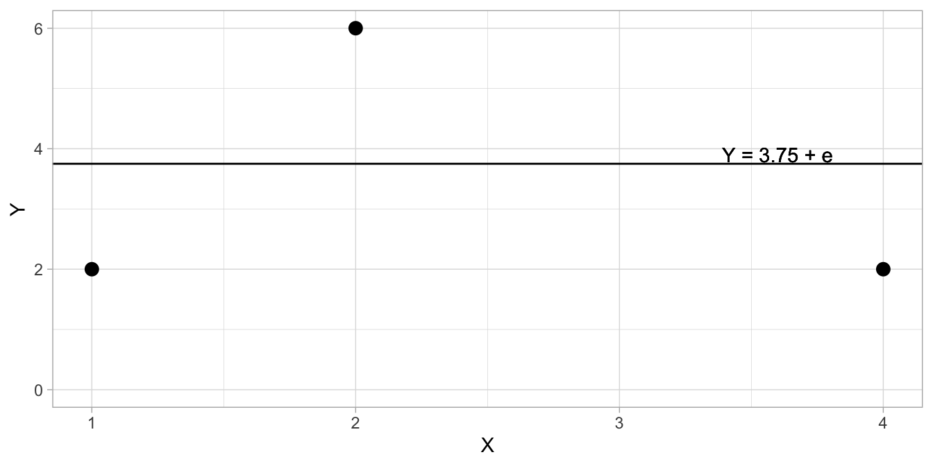
Figure 5.8: Illustration of residual degrees of freedom in a linear model, in case there is no slope and the intercept equals 3.75.

Before we continue, you must know that if we talk about degrees of freedom in regression analysis, we generally talk about residual degrees of freedom. We therefore look at residuals. If we compute the residuals, we have residuals -1.75, 2.25 and -1.75 for these data points. When we sum them, we get -1.25. Since we know that all residuals should sum to 0 in a regression analysis (see Chap. 4), we can derive the fourth residual to be +1.25, since only then the residuals sum to 0. Therefore, the $Y$-value for the fourth data point (for $X=3$) has to be 5, since then the residual is equal to $5 - 3.75 = 1.25$.

In short, when we use a linear model with only an intercept, the degrees of freedom is equal to the number of data points (combinations of $X$ and $Y$) minus 1, or in short notation: $n-1$, where $n$ stands for sample size.

Now let’s look at the situation where we use a linear model with both an intercept and a slope: suppose the intercept is equal to 3 and the slope is equal to 1: $Y=3+1 X+e$. Then suppose we have the same $X$-values as the example above: 1, 2 and 4. When we give these $X$-values corresponding $Y$-values, 2, 6, and 2, we get the plot in Figure 5.9.

Illustration of residual degrees of freedom, in case of a linear model with both intercept and slope for four data points (black line). The blue line is the regression line only using the three known data points.

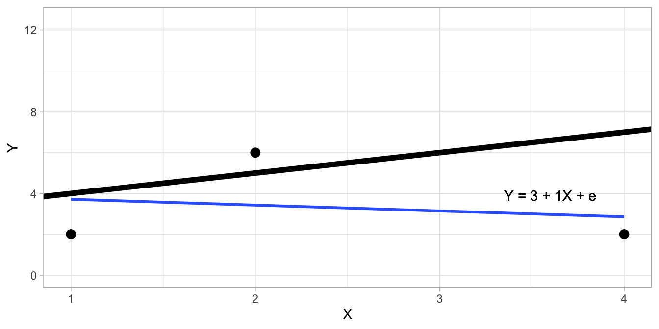
Figure 5.9: Illustration of residual degrees of freedom, in case of a linear model with both intercept and slope for four data points (black line). The blue line is the regression line only using the three known data points.

The black line is the regression line that we get when we analyse the complete data set of four points, $Y=3+1 X$. The blue line is the regression line based on only the three visible data points. Now the question is, is it possible for a fourth data point with $X=3$, to think of a $Y$-value such that the regression line based on these four data points is equal to $Y=3+1X$? In other words, can we choose a $Y$-value such that the blue line exactly overlaps with the black line?

Figure 5.10 shows a number of possibilities for the value of $Y$ if $X=3$. It can be seen, that it is impossible to pick a value for $Y_3$ such that we get a regression equation $Y=3+1X$. The blue line and green line intersect the black line at $X = 1$, but they have slopes that are less steep than the black line. If you use lower values for $Y$ such as 9 (red line) or higher values like 15 (purple line), the regression lines still do not overlap. It turns out to be impossible to choose a value for $Y_3$ in such a way that the regression line matches $Y=3+1X$.

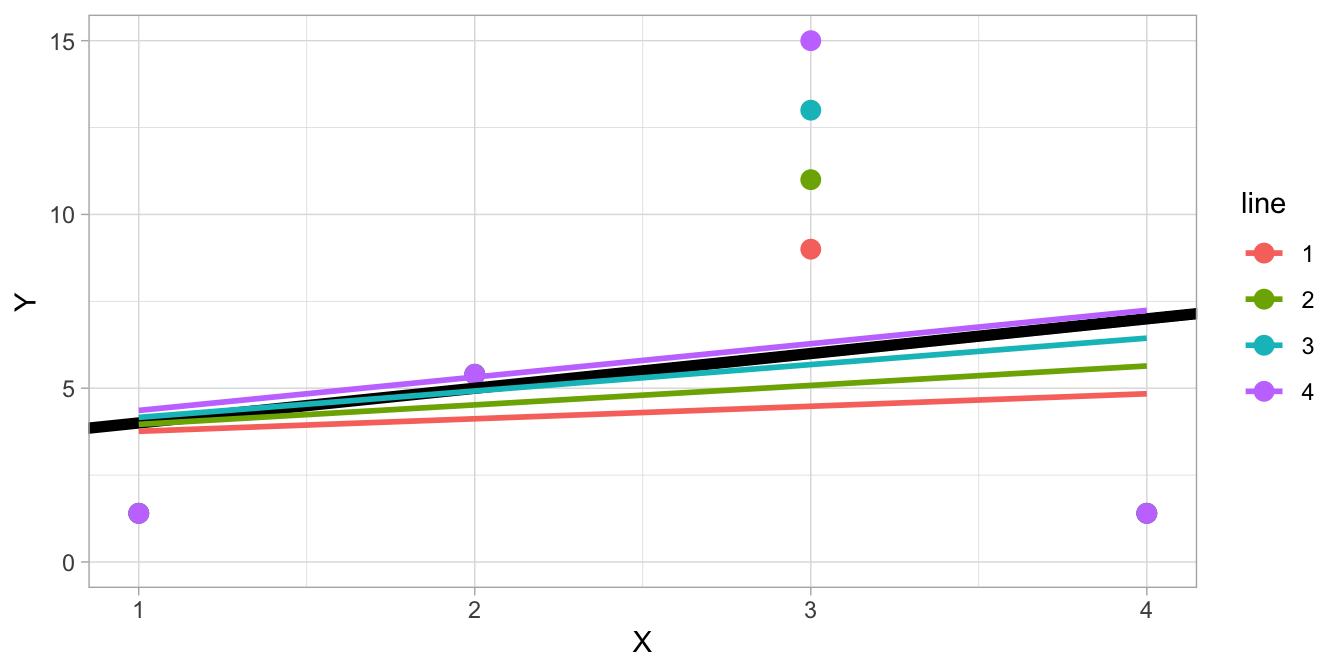
Figure 5.10: Different regression lines for different values of $Y$ if $X=3$.

So, with sample size $n=4$, we can never freely choose 3 residuals in order to satisfy the constraint that a particular regression equation holds for all 4 data points. We have less than 3 degrees of freedom because it is impossible to think of a fitting fourth value. It turns out, that in this case we can only choose 2 residuals freely, and the remaining residuals are then already determined. To prove this requires matrix algebra, but you can see it when you try it yourself.

The gist of it is that if you have a regression equation with both an intercept and a slope, the degrees of freedom is equal to the number of data points (sample size) minus 2: $n-2$. Generalising this to linear models with $K$ predictors: $n-K-1$.

Generally, these degrees of freedom based on the number of residuals that could be freely chosen, given the constraints of the model, are termed residual degrees of freedom. When using regression models, one usually only reports these residual degrees of freedom. Later on in this book, we will see instances where one also should use model degrees of freedom. For now, it suffices to know what is meant by residual degrees of freedom.

5.6 Null-hypothesis testing with linear models

Often, data analysis is about finding an answer to the question whether there is a relationship between two variables. In most cases, the question pertains to the population: is there a relationship between variable $Y$ and variable $X$ in the population? In many cases, one looks for a linear relationship between two variables.

One common method to answer this question is to analyse a sample of data, apply a linear model, and look at the slope. However, one then knows the slope in the sample, but not the slope in the population. We have seen that the slope in the sample can be very different from the slope in the population. Suppose we find a slope of 1: does that mean there is a slope in the population or that there is no slope in the population?

In inferential data analysis, one often works with two hypotheses: the null-hypothesis and the alternative hypothesis. The null-hypothesis states that the population slope is equal to 0 and the alternative hypothesis states that there is a slope that is different from 0. Remember that if the population slope is equal to 0, that is saying that there is no linear relationship between $X$ and $Y$ (that is, you cannot predict one variable on the basis of the other variable). Therefore, the null-hypothesis states there is no linear relationship between $X$ and $Y$ in the population. If there is a slope, whether positive or negative, is the same as saying there is a linear relationship, so the alternative hypothesis states that there is a linear relationship between $X$ and $Y$ in the population.

In formula form, we have

\[\begin{aligned} H_0: \beta_{slope}=0 \nonumber\\ H_A: \beta_{slope} \neq 0\nonumber \end{aligned}\]

The population slope, $\beta_{slope}$, is either 0 or it is not. Our data analysis is then aimed at determining which of these two hypotheses is true. Key is that we do a thought experiment on the null-hypothesis: we wonder what would happen if the population slope would be really 0. In our imagination we draw many samples of a certain size, say 40 data points, from a population where the slope is 0, and then determine the slope for each sample. Earlier we learned that the many sample slopes would form a histogram in the shape of a $t$-distribution with $n-2=38$ degrees of freedom. For example, suppose we would draw 1000 samples of size 40, then the histogram of the 1000 slopes would look like depicted Figure 5.11.

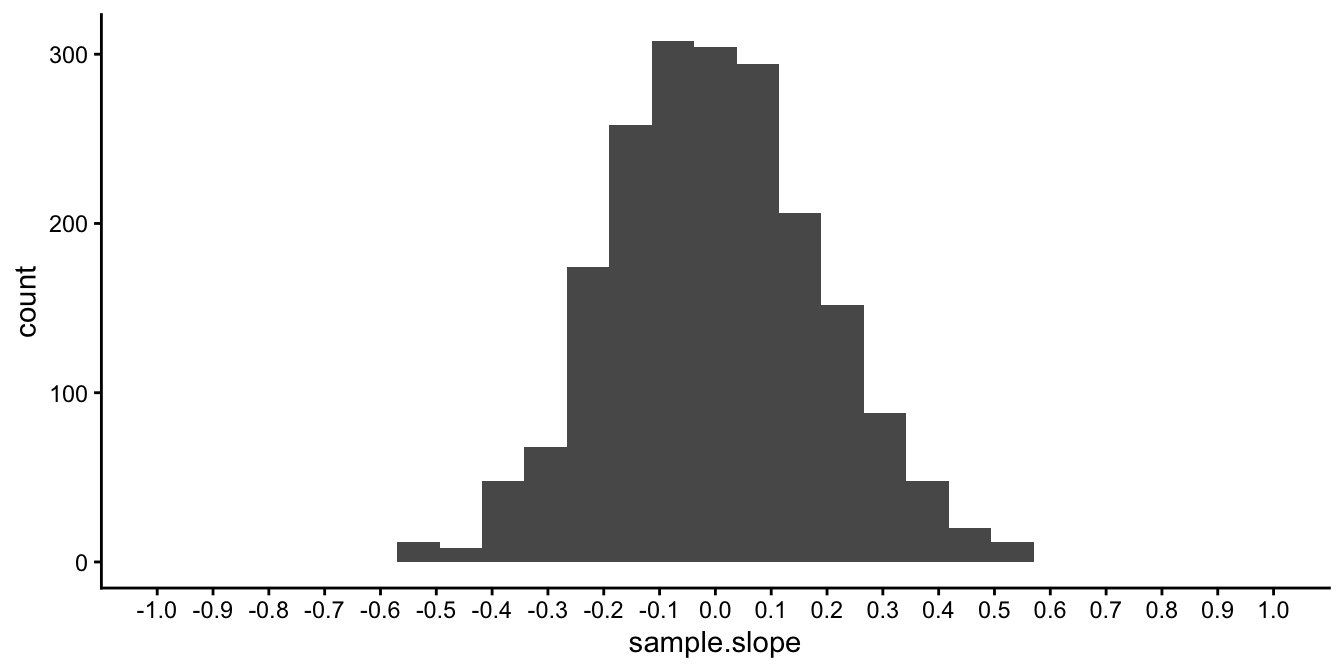
Figure 5.11: Distribution of the sample slope when the population slope is 0 and sample size equals 40.

From this histogram we see that all observed sample slopes are well between -0.8 and 0.8. This gives us the information we need. Of course, we have only one sample of data, and we don’t know anything about the population data. But we do know that if the population slope is equal to 0, then it is very unlikely to find a sample slope of say 1 or -1. Thus, with our sample slope of 1, we know that this finding is very unlikely if we hold the null-hypothesis to be true. In other words, if the population slope is equal to 0, it would be quite improbable to find a sample slope of 1 or larger. Therefore, we regard the null-hypothesis to be false, since it does not provide a good explanation of why we found a sample slope of 1. In that case, we say that we reject the null-hypothesis. We say that the slope is significantly different from 0, or simply that the slope is significant.

5.7 $p$-values

A $p$-value is a probability. It represents the probability of observing certain events, given that the null-hypothesis is true.

In the previous section we saw that if the population slope is 0, and we drew 1000 samples of size 40, we did not observe a sample slope of 1 or larger. In other words, the frequency of observing a slope of 1 or larger was 0. If we would draw more samples, we theoretically could observe a sample slope of 1 or larger, but the probability that that happens for any new sample we can estimate at less than 1 in a 1000, so less than 0.001: $p < 0.001$.

This estimate of the $p$-value was based on 1000 randomly drawn samples of size 40 and then looking at the frequency of certain values in that data set. But there is a short-cut, for we know that the distribution of sample slopes has a $t$-distribution if we standardise the sample slopes. Therefore we do not have to take 1000 samples and estimate probabilities, but we can look at the $t$-distribution directly, using tables online or in statistical packages.

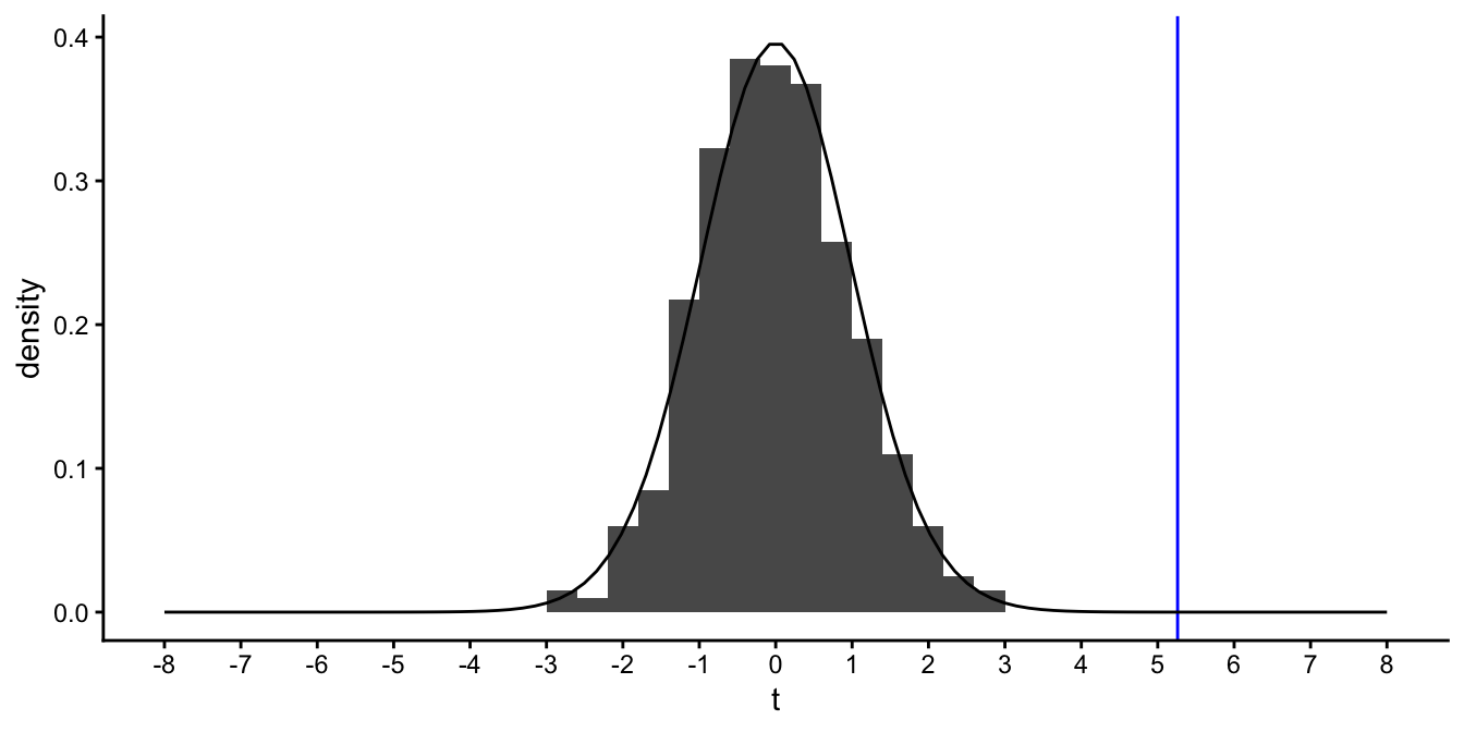
The histogram of 1000 sample slopes and its corresponding theoretical $t$-distribution with 38 degrees of freedom. The vertical blue line represents the $t$-value of 5.26.

Figure 5.12: The histogram of 1000 sample slopes and its corresponding theoretical $t$-distribution with 38 degrees of freedom. The vertical blue line represents the $t$-value of 5.26.

Figure 5.12 shows the $t$-distribution that is the theoretical distribution corresponding to the histogram in Figure 5.11. If the standard error is equal to 0.19, and the hypothetical population slope is 0, then the $t$-statistic associated with a slope of 1 is equal to $t=\frac{1-0}{0.19}=5.26$. With this value, we can look up in the tables, how often such a value of 5.26 or larger occurs in a $t$-distribution with 38 degrees of freedom. In the tables or using R, we find that the probability that this occurs is 0.00000294.

1 - pt(5.26, df = 38)

## [1] 2.939069e-06

So, the fact that the $t$-statistic has a $t$-distribution gives us the opportunity to exactly determine certain probabilities, including the $p$-value.

Now let’s suppose we have only one sample of 40 bottles, and we find a slope of 0.1 with a standard error of 0.19. Then this value of 0.1 is $(0.1-0)/0.19=0.53$ standard errors away from 0. Thus, the $t$-statistic is 0.53. We then look at the $t$-distribution with 38 degrees of freedom, and see that such a $t$-value of 0.53 is not very strange: it lies well within the middle 95% of the $t$-distribution (see Figure 5.12).

Let’s determine the $p$-value again for this slope of 0.1: we determine the probability that we obtain such a $t$-value of 0.53 or larger. Figure 5.13 shows the area under the curve for values of $t$ that are larger than 0.53. This area under the curve can be seen as a probability. The total area under the curve of the $t$-distribution amounts to 1. If we know the area of the shaded part of the total area, we can compute the probability of finding $t$-values larger than 0.53.

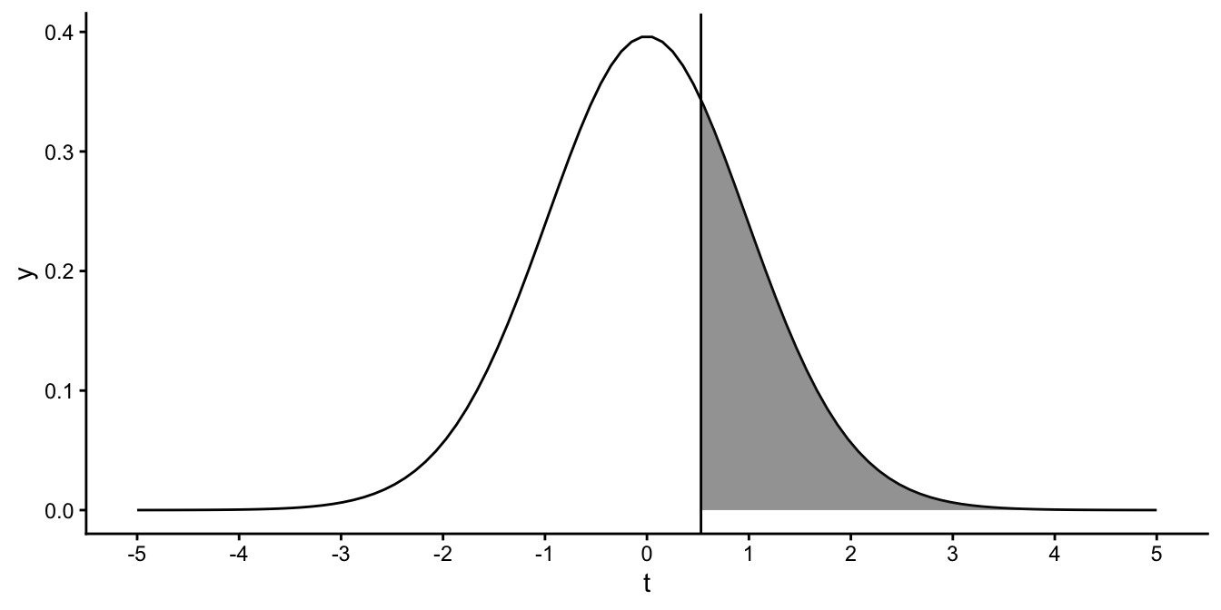
Figure 5.13: Probability of a $t$-value larger than 0.53.

In tables online, in Appendix B, or available in statistical packages, we can look up how large this area is. It turns out to be 0.3.

1 - pt(0.53, df = 38)

## [1] 0.2995977

So, if the population slope is equal to 0 and we draw an infinite number of samples of size 40 and compute the sample slopes, then 30% of them will be larger than our sample slope of 0.1. The proportion of the shaded area is what we call a one-sided $p$-value. We call it one-sided, because we only look at one side of the $t$-distribution: we only look at values that are larger than our $t$-value of 0.53.

We conclude that a slope value of 0.1 is not that strange to find if the population slope is 0. By the same token, it would also have been probable to find a slope of -0.1, corresponding to a $t$-value of -0.53. Since the $t$-distribution is symmetrical, the probability of finding a $t$-value of less than -0.53 is depicted in Figure 5.14, and of course this probability is also 0.3.

pt(-0.53, df = 38)

## [1] 0.2995977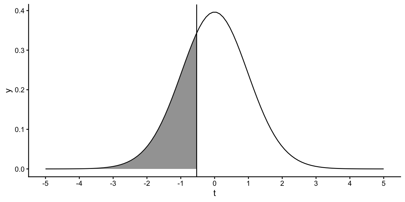

Figure 5.14: Probability of finding a $t$-value smaller than -0.53.

Remember that the null-hypothesis is that the population slope is 0, and the alternative hypothesis is that the population slope is not 0. We should therefore conclude that if we find a very large positive or negative slope, large in the sense of the number of standard errors away from 0, that the null-hypothesis is unlikely to be true. Therefore, if we find a slope of 0.1 or -0.1, then we should determine the probability of finding a $t$-value that is larger than 0.53 or smaller than -0.53. This probability is depicted in Figure 5.15 and is equal to twice the one-side $p$-value, $2 \times 0.2995977=0.5991953$.

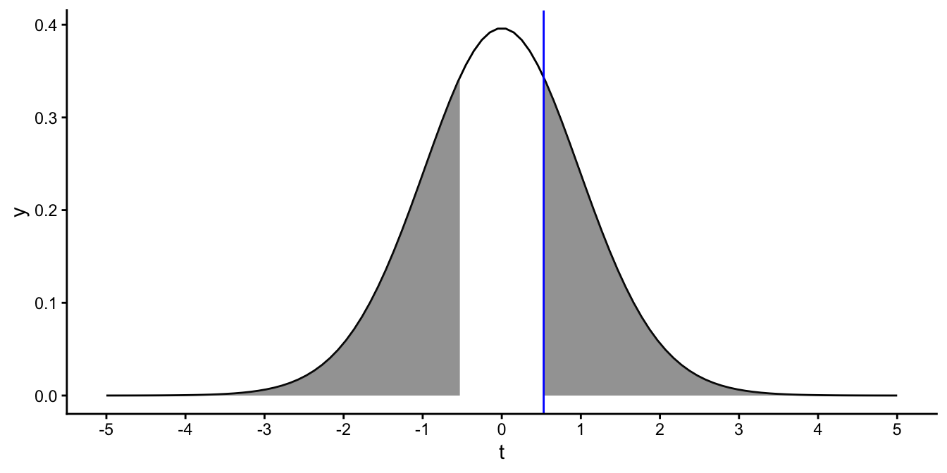
The blue vertical line represents a $t$-value of 0.53. The shaded area represents the two-sided $p$-value: the probability of obtaining a $t$-value smaller than -0.53 or larger than 0.53.

Figure 5.15: The blue vertical line represents a $t$-value of 0.53. The shaded area represents the two-sided $p$-value: the probability of obtaining a $t$-value smaller than -0.53 or larger than 0.53.

This probability is called the two-sided $p$-value. This is the one that should be used, since the alternative hypothesis is also two-sided: the population slope can be positive or negative. The question now is: is a sample slope of 0.1 enough evidence to reject the null-hypothesis? To determine that, we determine how many standard errors away from 0 the sample slope is and we look up in tables how often that happens. Thus in our case, we found a slope that is 0.53 standard errors away from 0 and the tables told us that the probability of finding a slope that is at least 0.53 standard errors away from 0 (positive or negative) is equal to 0.5991953. We find this probability rather large, so we decide that we do not reject the null-hypothesis.

5.8 Hypothesis testing

In the previous section, we found a one-sided $p$-value of 0.00000294 for a sample slope of 1 and more or less concluded that this probability was rather small. The two-sided $p$-value would be twice this value, so 0.00000588, which is still very small. Next, we determined the $p$-value associated with a slope of 0.1 and found a $p$-value of 0.60. This probability was rather large, and we decided to not reject the null-hypothesis. In other words, the probability was so large that we thought that the hypothesis that the population slope is 0 should not be rejected based on our findings.

When should we think the $p$-value is small enough to conclude that the null-hypothesis can be rejected? When can we conclude that the hypothesis that the population slope is 0 is not supported by our sample data? This was a question posed to the founding father of statistical hypothesis testing, Sir Ronald Fischer. In his book Statistical Methods for Research Workers (1925), Fisher proposed a probability of 5%. He advocated 5% as a standard level for concluding that there is evidence against the null-hypothesis. However, he did not see it as an absolute rule: "If P is between .1 and .9 there is certainly no reason to suspect the hypothesis tested. If it is below .02 it is strongly indicated that the hypothesis fails to account for the whole of the facts. We shall not often be astray if we draw a conventional line at .05...". So Fisher saw the $p$-value as an informal index to be used as a measure of discrepancy between the data and the null-hypothesis: The null-hypothesis is never proved, but is possibly disproved.

Later, Jerzy Neyman and Egon Pearson saw the $p$-value as an instrument in decision making: is the null-hypothesis true, or is the alternative hypothesis true? You either reject the null-hypothesis or you don’t, there is nothing in between. A slightly milder view is that you either decide that there is enough empirical evidence to reject the null-hypothesis, or there is not enough empirical evidence to reject the null-hypothesis (not necessarily accepting $H_0$ as true!). This view to data-analysis is rather popular in the social and behavioural sciences, but also in particle physics. In order to make such black-and-white decisions, you decide before-hand, that is, before collecting data, what level of significance you choose for your $p$-value to decide whether to reject the null-hypothesis. For example, as your significance level, you might want to choose 1%. Let’s call this chosen significance level $\alpha$. Then you collect your data, you apply your linear model to the data, and find that the $p$-value associated with the slope equals $p$. If this $p$ is smaller than or equal to $\alpha$, you reject the null-hypothesis, and if $p$ is larger than $\alpha$ then you do not reject the null-hypothesis. A slope with a $p \leq \alpha$ is said to be significant, and a slope with a $p > \alpha$ is said to be non-significant. If the sample slope is significant, then one should reject the null-hypothesis and say there is a slope in the population different from zero. If the sample slope is not significant, then one should not reject the null-hypothesis (i.e., the population slope could well be 0). One could say there is no empirical evidence for the existence of a slope not equal to 0. This leaves the possibility that there is a slope in the population, but that our method of research failed to find evidence for it. Formally, the null-hypothesis testing framework only allows refuting a null-hypothesis by some empirical evidence. It does not allow you to prove that the null-hypothesis is true, only that the null-hypothesis being true is a possibility.

5.9 Inference for linear models in R

So far, we have focused on standard errors and confidence intervals for the slope parameter in simple regression, that is, a linear model where there is only one independent variable. However, the same logic can be applied to the intercept parameter, and to other slope variables in case you have multiple independent variables in your model (multiple regression).

For instance, suppose we are interested in the knowledge university students have of mathematics. We start measuring their knowledge at time 0, when the students start doing a bachelor programme in mathematics. At time 1 (after 1 year) and at time 2 (after two years), we also perform measures. Our dependent variable is mathematical knowledge, a measure with possible values between 200 and 700. The independent variables are time (the time of measurement) and distance: the distance in kilometres between university and their home. There are two research questions. The first question is about the level of knowledge when students enter the bachelor programme, and the second question is how much knowledge is acquired in one year of study. The linear model is as follows:

\[\begin{aligned} \texttt{knowledge} &= b_0 + b_1 \texttt{time} + b_2 \texttt{distance} + e \nonumber\\ e &\sim N(0, \sigma^2) \nonumber\end{aligned}\]

Table 5.2: Regression table as obtained from R, with knowledge predicted by time and distance.
term	estimate	std.error	statistic	p.value
(Intercept)	299.35	7.60	39.40	0.00
time	18.13	2.60	6.96	0.00
distance	-0.76	0.67	-1.15	0.25

The first question could be answered by estimating the intercept $b_0$: that is the level of knowledge we expect for a student at time 0 and with a home 0 kilometres from the university. The second question could be answered by estimating the slope coefficient for time: the expected increase in knowledge per year. In Chapter 4 we saw how to estimate the regression parameters in R. We saw that we then get a regression table. For our mathematical knowledge example, we could obtain the regression table, displayed in Table 5.2. We discussed the first column with the regression parameters in Chapter 4. We see that the intercept is estimated at 299.35, and the slopes for time and distance are 18.13 and -0.76, respectively. So we can fill in the equation:

\[\begin{aligned} \texttt{knowledge} = 299.35 + 18.13 \texttt{time} -0.76 \texttt{distance} + e \nonumber \end{aligned}\]

Let’s look at the other columns in the regression table. In the second column we see the standard errors for each parameter. The third column gives statistics; these are the $t$-statistics for the null-hypotheses that the respective parameters in the population are 0. For instance, the first statistic has the value 39.40. It belongs to the intercept. If the null-hypothesis is that the population intercept is 0 ($\beta_0 = 0$), then the $t$-statistic is computed as

\[t = \frac{b_0 - \beta_0}{\sigma_{\hat{\beta}}} =\frac{ 299.35 - 0 }{7.60} = \frac{ 299.35 }{7.60} = 39.40\]

You see that the $t$-statistic in the regression table is simply the regression parameter divided by its standard error. This is also true for the slope parameters. For instance, the $t$-statistic of 6.96 for time is simply the regression coefficient 18.13 divided by the standard error 2.60:

\[t = \frac{b_1 - \beta_0}{\sigma_{\hat{\beta}}} =\frac{ 18.13 - 0 }{7.60} = \frac{ 18.13 }{2.60} = 6.96\]

The last column gives the two-sided $p$-values for the respective null-hypotheses. For instance, the $p$-value of 0.00 for the intercept says that the probability of finding an intercept of 299.35 or larger (plus or minus), under the assumption that the population intercept is 0, is very small (less than 0.01).

If you want to have confidence intervals for the intercept and the slope for time, you can use the information in the table to construct them yourself. For instance, according to the table, the standard error for the intercept equals 7.60. Suppose the sample size equals 90 students, then you know that you have $n-K-1 = 90 - 2 - 1 = 87$ degrees of freedom. The critical value for a $t$-statistic with 84 degrees of freedom for a 95% confidence interval can be looked up in Appendix B. It must be somewhere between 1.98 and 2.00, so let’s use 1.99. The 95% interval for the intercept then runs between $299.35 - 1.99 \times 7.60$ and $299.35 - 1.99 \times 7.60$, so the expected level of knowledge at the start of the bachelor programme for students living close to or on campus is somewhere between from 284.23 to 314.47.

To show you how this can all be done using R, we have a look at the R dataset called "freeny" on quarterly revenues. We would like to predict the variable market.potential by the predictors price.index and income.level. Apart from the tidyverse package, we also need the broom package for the tidy() function. When we run the following code, we obtain a regression table.

library(broom)
data("freeny")
out <- freeny %>% 
  lm(market.potential ~ price.index + income.level, data = .)
out %>% 
  tidy()

## # A tibble: 3 × 5
##   term         estimate std.error statistic  p.value
##   <chr>           <dbl>     <dbl>     <dbl>    <dbl>
## 1 (Intercept)    13.3      0.291      45.6  1.86e-33
## 2 price.index    -0.309    0.0263    -11.8  6.92e-14
## 3 income.level    0.196    0.0291      6.74 7.20e- 8

We can have R compute the respective confidence intervals by indicating that we want intervals of a certain confidence level, say 99%:

out <- freeny %>% 
  lm(market.potential ~ price.index + income.level, data = .) 
out %>% 
  tidy(conf.int = TRUE, conf.level = 0.99)

## # A tibble: 3 × 7
##   term         estimate std.error statistic  p.value conf.low conf.high
##   <chr>           <dbl>     <dbl>     <dbl>    <dbl>    <dbl>     <dbl>
## 1 (Intercept)    13.3      0.291      45.6  1.86e-33   12.5      14.1  
## 2 price.index    -0.309    0.0263    -11.8  6.92e-14   -0.381    -0.238
## 3 income.level    0.196    0.0291      6.74 7.20e- 8    0.117     0.276

freeny$market.potential %>% length()

## [1] 39

In the last two columns we see for example that the 99% confidence interval for the price.index slope runs from -0.381 to -0.238.

We can report:

"In a multiple regression of market potential on price index and income level ($N = 39$), we found a slope for price index of -0.309 (SE = 0.026, 99% CI: -0.381, -0.238)."

5.10 Type I and Type II errors in decision making

Since data analysis is about probabilities, there is always a chance that you make the wrong decision: you can wrongfully reject the null-hypothesis, or you can wrongfully fail to reject the null-hypothesis. Pearson and Neyman distinguished between two kinds of error: one could reject the null-hypothesis while it is actually true (error of the first kind, or type I error) and one could accept the null-hypothesis while it is not true (error of the second kind, or type II error). We already discussed these types of error in Chapter 2. The table below gives an overview.

Four different scenarios for hypothesis tests.
	Test conclusion
	do not reject $H_0$	reject $H_0$
$H_0$ true	OK	Type I Error
$H_A$ true	Type II Error	OK

To illustrate the difference between type I and type II errors, let’s recall the famous fable by Aesop about the boy who cried wolf. The tale concerns a shepherd boy who repeatedly tricks other people into thinking a wolf is attacking his flock of sheep. The first time he cries "There is a wolf!", the men working in an adjoining field come to help him. But when they repeatedly find there is no wolf to be seen, they realise they are being fooled by the boy. One day, when a wolf does appear and the boy again calls for help, the men believe that it is another false alarm and the sheep are eaten by the wolf.

In this fable, we can think of the null-hypothesis as the hypothesis that there is no wolf. The alternative hypothesis is that there is a wolf. Now, when the boy cries wolf the first time, there is in fact no wolf. The men from the adjoining field make a type I error: they think there is a wolf while there isn’t. Later, when they are fed up with the annoying shepherd boy, they don’t react when the boy cries "There is a wolf!". Now they make a type II error: they think there is no wolf, while there actually is a wolf. The table below gives an overview.

Four different scenarios for wolves and men working in the field.
	Men in the field
	Think there is no wolf	Think there is a wolf
There is no wolf	OK	waste of time and energy
There is a wolf	devoured sheep	OK

Let’s now discuss these errors in the context of linear models. Suppose you want to determine the slope for the effect of age on height in children. Let the slope now stand for the wolf: either there is no slope (no wolf, $H_0$) or there is a slope (wolf, $H_A$). The null-hypothesis is that the slope is 0 in the population of all children (a slope of 0 means there is no slope) and the alternative hypothesis that the slope is not 0, so there is a slope. You might study a sample of children and you might find a certain slope. You might decide that if the $p$-value is below a critical value you conclude that the null-hypothesis is not true. Suppose you think a probability of 10% is small enough to reject the null-hypothesis as true. In other words, if $p \leq 0.10$ then we no longer think 0 is a reasonable value for the population slope. In this case, we have fixed our $\alpha$ or type I error rate to be $\alpha=0.10$. This means that if we study a random sample of children, we look at the slope and find a $p$-value of 0.11, then we do not reject the null-hypothesis. If we find a $p$-value of 0.10 or less, then we reject the null-hypothesis.

Note that the probability of a type I error is the same as our $\alpha$ for the significance level. Suppose we set our $\alpha=0.05$. Then for any $p$-value equal or smaller than 0.05, we reject the null-hypothesis. Suppose the null-hypothesis is true, how often do we then find a $p$-value smaller than 0.05? We find a $p$-value smaller than 0.05 if we find a $t$-value that is above a certain threshold. For instance, for the $t$-distribution with 198 degrees of freedom, the critical value is $\pm 1.97$, because only in 5% of the cases we find a $t$-value of $\pm 1.97$ or more if the null-hypothesis is true! Thus, if the null-hypothesis is true, we see a $t$-value of at least $\pm 1.97$ in 5% of the cases. Therefore, we see a significant $p$-value in 5% of the cases if the null-hypothesis is true. This is exactly the definition of a type I error: the probability that we reject the null-hypothesis (finding a significant $p$-value), given that the null-hypothesis is true. So we call our $\alpha$-value the type I error rate.

Suppose 100 researchers are studying a particular slope. Unbeknownst to them, the population slope is exactly 0. They each draw a random sample from the population and test whether their sample slope is significantly different from 0. Suppose they all use different sample sizes, but they all use the same $\alpha$ of 0.05. Then we can expect that about 5 researchers will reject the null-hypothesis (finding a $p$-value less than or smaller than 0.05) and about 95 will not reject the null-hypothesis (finding a $p$-value of more than 0.05).

Fixing the type I error rate should always be done before data collection. How willing are you to take a risk of a type I error? You are free to make a choice about $\alpha$, as long as you do it before looking at the data, and report what value you used.

If $\alpha$ represents the probability of making a type I error, then we can use $\beta$ to represent the opposite: the probability of not rejecting the null-hypothesis while it is not true (type II error, thinking there is no wolf while there is). However, setting the $\beta$-value prior to data collection is a bit trickier than choosing your $\alpha$. It is not possible to compute the probability that we find a non-significant effect $(p > \alpha)$, given that the alternative hypothesis is true, because the alternative hypothesis is only saying that the slope is not equal to 0. In order to compute $\beta$, we need to think first of a reasonable size of the slope that we expect. For example, suppose we believe that a slope of 1 is quite reasonable, given what we know about growth in children. Let that be our alternative hypothesis:

\[\begin{aligned} H_0: \beta_1 =0 \nonumber \\ H_A: \beta_1 = 1\nonumber\end{aligned}\]

Next, we determine the distribution of sample slopes under the assumption that the population slope is 1. We know that this distribution has a mean of 1 and a standard deviation equal to the standard error. We also know it has the shape of a $t$-distribution. Let sample size be equal to 102 and the standard error 2. If we standardise the slopes by dividing by the standard error, we get the two $t$-distributions in Figure 5.16: one distribution of $t$-values if the population slope is 0 (centred around $t=0$), and one distribution of $t$-values if the population slope is 1 (centred around $t=1/2=0.5$).

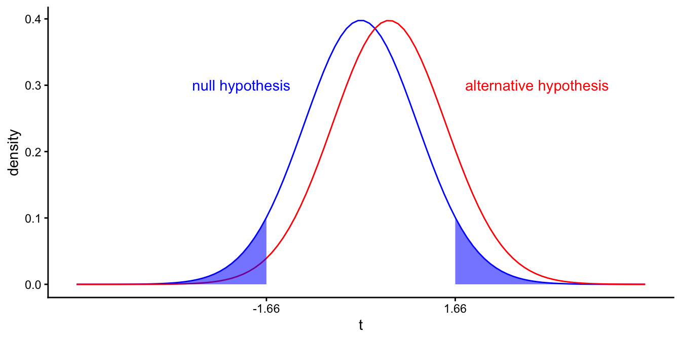
$Different $t$-distributions of the sample slope if the population slope equals 0 (left curve in blue), and if the population slope equals 1 (right curve in red). Blue area depicts the probability that we find a $p$-value value smaller than 0.10 if the population slope is 0 ($\alpha$).$

Figure 5.16: Different $t$-distributions of the sample slope if the population slope equals 0 (left curve in blue), and if the population slope equals 1 (right curve in red). Blue area depicts the probability that we find a $p$-value value smaller than 0.10 if the population slope is 0 ($\alpha$).

Let’s fix $\alpha$ to 10%. The shaded areas represent the area where $p \leq \alpha$: for all values of $t$ smaller than $-1.6859545$ and larger than $1.6859545$, we reject the null-hypothesis. The probability that this happens, if the null-hypothesis is true, is equal to $\alpha$, which is 0.10 in this example. The probability that this happens if the alternative hypothesis is true (i.e., population slope is 1), is depicted in Figure @(fig:inf_21).

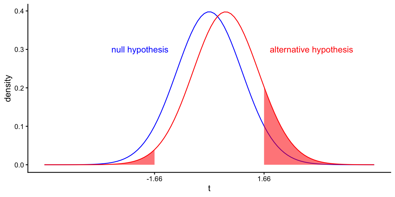
$Different $t$-distributions of the sample slope if the population slope equals 0 (left curve in blue), and if the population slope equals 1 (right curve in red). Shaded area depicts the probability that we find a $p$-value value smaller than 0.10 if the population slope is 1 ($1-\beta$).$

Figure 5.17: Different $t$-distributions of the sample slope if the population slope equals 0 (left curve in blue), and if the population slope equals 1 (right curve in red). Shaded area depicts the probability that we find a $p$-value value smaller than 0.10 if the population slope is 1 ($1-\beta$).

The shaded area in Figure 5.17 turns out to be $0.1415543$. This represents the probability that we find a significant effect, if the population slope is 1. This is actually 1 minus the probability of finding a non-significant effect, if the population slope is 1, which is defined as $\beta$. Therefore, the shaded area in Figure 5.17 represents $1- \beta$: the probability of finding a significant $p$-value, if the population slope is 1. In this example, $1-\beta$ is equal to $0.1415543$, so $\beta$ is equal to $1- 0.1415543 = 0.8584457$.

In sum, in this example with an $\alpha$ of 0.10 and assuming a population slope of 1, we find that the probability of a type II error is 0.86: if there is a slope of 1, then we have an 86% chance of wrongly concluding that the slope is 0.

Type I and II error rates $\alpha$ and $\beta$ are closely related. If we feel that a significance level of $\alpha=0.10$ is too high, we could choose a level of 0.01. This ensures that we are less likely to reject the null-hypothesis when it is true. The critical value for our $t$-statistic is then equal to $\pm 2.6258905$, see Figure 5.18. In Figure 5.19 we see that if we change $\alpha$, we also get a different value for $1-\beta$, in this case $0.0196567$.

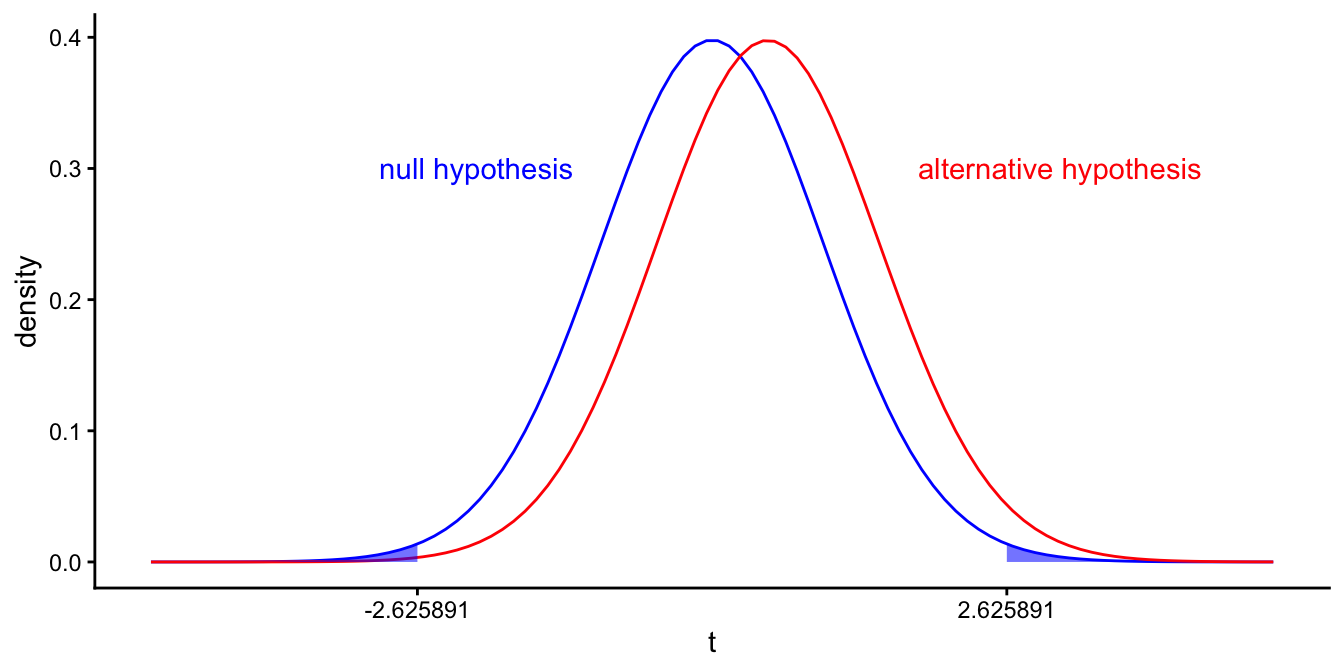
Different $t$-distributions of the sample slope if the population slope equals 0 (left curve), and if the population slope equals 1 (right curve). Blue area depicts the probability that we find a $p$-value value smaller than 0.01 if the population slope is 0.

Figure 5.18: Different $t$-distributions of the sample slope if the population slope equals 0 (left curve), and if the population slope equals 1 (right curve). Blue area depicts the probability that we find a $p$-value value smaller than 0.01 if the population slope is 0.

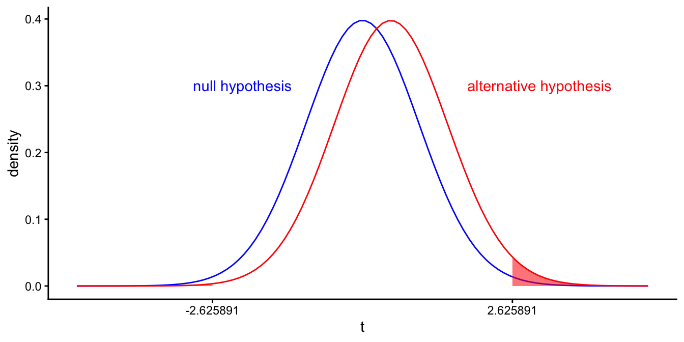
$Different $t$-distributions of the sample slope if the population slope equals 0 (left curve in blue), and if the population slope equals 1 (right curve in red). Red area depicts the probability that we find a $p$-value value smaller than 0.01 if the population slope is 1: $1-\beta$.$

Figure 5.19: Different $t$-distributions of the sample slope if the population slope equals 0 (left curve in blue), and if the population slope equals 1 (right curve in red). Red area depicts the probability that we find a $p$-value value smaller than 0.01 if the population slope is 1: $1-\beta$.

The table below gives an overview of how $\alpha$ and $\beta$ are related to type I and type II error rates. If a $p$-value for a statistical test is equal to or smaller than a pre-chosen significance level $\alpha$, the probability of a type I error equals $\alpha$. The probability of a type II error rate is equal to $\beta$.

The probabilities of a statistical outcome under the null-hypothesis and the alternative hypothesis.
	Statistical outcome
	$p > \alpha$	$p \leq \alpha$
$H_0$	$1-\alpha$	$\alpha$
$H_A$	$\beta$	$1-\beta$

Thus, if we use smaller values for $\alpha$, we get smaller values for $1-\beta$, so we get larger values for $\beta$. This means that if we lower the probability of rejecting the null-hypothesis given that it is true (type I error) by choosing a lower value for $\alpha$, we inadvertently increase the probability of failing to reject the null-hypothesis given that it is not true (type II error).

Think again about the problem of the sheep and the wolf. Instead of the boy, the men could choose to put a very nervous person on watch, someone very scared of wolves. With the faintest hint of a wolf’s presence, the man will call out "Wolf!". However, this will lead to many false alarms (type I errors), but the men will be very sure that when there actually is a wolf, they will be warned. Alternatively, they could choose to put a man on watch that is very laid back, very relaxed, but perhaps prone to nod off. This will lower the risk of false alarms immensely (no more type I errors) but it will dramatically increase the risk of a type II error!

One should therefore always strike a balance between the two types of errors. One should consider how bad it is to think that the slope is not 0 while it is, and how bad it is to think that the slope is 0, while it is not. If you feel that the first mistake is worse than the second one, then make sure $\alpha$ is really small, and if you feel that the second mistake is worse, then make $\alpha$ not too small. Another option, and a better one, to avoid type II errors, is to increase sample size, as we will see in the next section.

5.11 Statistical power

Null-hypothesis testing only involves the null-hypothesis: we look at the sample slope, compute the $t$-statistic and then see how often such a $t$-value and larger values occur given that the population slope is 0. Then we look at the $p$-value and if that $p$-value is smaller than or equal to $\alpha$, we reject the null-hypothesis. Therefore, null-hypothesis testing does not involve testing the alternative hypothesis. We can decide what value we choose for our $\alpha$, but not our $\beta$. The $\beta$ is dependent on what the actual population slope is, and we simply don’t know that.

As stated in the previous section, we can compute $\beta$ only if we have a more specific idea of an alternative value for the population slope. We saw that we needed to think of a reasonable value for the population slope that we might be interested in. Suppose we have the intuition that a slope of 1 could well be the case. Then, we would like to find a $p$-value of less than $\alpha$ if indeed the slope were 1. We hope that the probability that this happens is very high: the conditional probability that we find a $t$-value large enough to reject the null-hypothesis, given that the population slope is 1. This probability is actually the complement of $\beta$, $1-\beta$: the probability that we reject the null-hypothesis, given that the alternative hypothesis is true. This $1-\beta$ is often called the statistical power of a null-hypothesis test. When we think again about the boy who cried wolf: the power is the probability that the men think there is a wolf if there is indeed a wolf. The power of a test should always be high: if there is a population slope that is not 0, then of course you would like to detect it by finding a significant $t$-value!

In order to get a large value for $1-\beta$, we should have large $t$-values in our data-analysis. There are two ways in which we can increase the value of the $t$-statistic. Since with null-hypothesis testing $t=\frac{b-0}{\sigma_{\hat{b}}}=\frac{b}{\sigma_{\hat{b}}}$, we can get large values for $t$ if 1) we have a small standard error, $\sigma_{\hat{b}}$, or 2) if we have a large value for $b$.

Let’s first look at the first option: a small standard error. We get a small standard error if we have a large sample size, see Section 5.2.1. If we go back to the example of the previous section where we had a sample size of 102 children and our alternative hypothesis was that the population slope was 1, we found that the $t$-distribution for the alternative hypothesis was centred around 0.5, because the standard error was 2. Suppose that we would increase sample size to 1200 children, then our standard error might be 0.2. Then our $t$-distribution for the alternative hypothesis is centred at 5. This is shown in Figure 5.20.

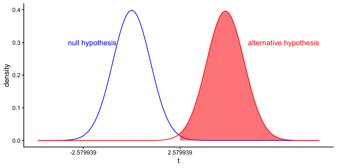
Different $t$-distributions of the sample slope if the population slope equals 0 (left curve in blue), and if the population slope equals 1 (right curve in red). Now for a larger sample size. Shaded area depicts the probability that we find a $p$-value value smaller than 0.01 if the population slope is 1.

Figure 5.20: Different $t$-distributions of the sample slope if the population slope equals 0 (left curve in blue), and if the population slope equals 1 (right curve in red). Now for a larger sample size. Shaded area depicts the probability that we find a $p$-value value smaller than 0.01 if the population slope is 1.

We see from the shaded area that if the population slope is really 1, there is a very high chance that the $t$-value for the sample slope will be larger than 2.58, the cut-off point for an $\alpha$ of 0.01 and 1198 degrees of freedom. The probability of rejecting the null-hypothesis while it is not true, is therefore very large. This is our $1-\beta$ and we call this the power of the null-hypothesis test. We see that with increasing sample size, the power to find a significant $t$-value increases too.

Now let us look at the second option, a large value of $b$. Sample slope $b_1$ depends of course on the population slope $\beta_1$. The power becomes larger when the population slope is further away from zero. If the population slope were 10, and we only had a sample of 102 children (resulting in a standard error of 2), the $t$-distribution for the alternative hypothesis that the population slope is centred around $\frac{b}{\sigma_{\hat{b}}}=10/2=5$, resulting in the same plot as in Figure 5.20, with a large value for $1-\beta$. Unfortunately, the population slope is beyond our control: the population slope is a given fact that we cannot change. The only thing we can change most of the times is sample size.

In sum: the statistical power of a test is the probability that the null-hypothesis is rejected, given that it is not true. This probability is equal to $1-\beta$. The statistical power of a test increases with sample size, and depends on the actual population slope. The further away the population slope is from 0 (positive or negative), the larger the statistical power. Earlier we also saw that $1-\beta$ increases with increasing $\alpha$: the larger $\alpha$, the higher the power.

5.12 Power analysis

Because of these relationships between statistical power, $\alpha$, sample size $n$, and the actual population slope $\beta_1$, we can compute the statistical power for any combination thereof.

If you really care about the quality of your research, you carry out a power analysis prior to collecting data. With such an analysis you can find out how large your sample size should be. You can find many tools online that can help you with that.

Suppose you want to minimise the probability of a type I error, so you choose an $\alpha=0.01$. Next, you think of what kind of population slope you would like to find, if it indeed has that value. You could perhaps base this expectation on earlier research. Suppose that you feel that if the population slope is 0.15, you would really like to find a significant $t$-value so that you can reject the null-hypothesis. Next, you have to specify how badly you want to reject the null-hypothesis if indeed the population slope is 0.15. If the population slope is really 0.15, then you would like to have a high probability to find a $t$-value large enough to reject the null-hypothesis. This is of course the power of the test, $1-\beta$. Let’s say you want to have a power of 0.90. Now you have enough information to calculate how large your sample size should be.

Let’s look at G*power²¹, an application that can be downloaded from the web. If we start the app, we can ask for the sample size required for a slope of 0.15, an $\alpha$ of 0.01, and a power ($1-\beta$) of 0.90. Let the standard deviation of our dependent variable ($Y$) be 3 and the standard deviation of our independent variable ($X$) be 2. These numbers you can guess, preferably based on some other data that were collected earlier. Then we get the input as displayed in Figure 5.21. Note that you should use two-sided $p$-values, so tails = two. From the output we see that the required sample size is 1477 children.

Figure 5.21: The G*power app interface.

5.13 Criticism on null-hypothesis testing and $p$-values

The practice of null-hypothesis significance testing (NHST) is widespread. However, from the beginning it has received much criticism. One of the first to criticise the approach was the inventor of the $p$-value, Sir Ronald Fisher himself. Fisher explicitly contrasted the use of the $p$-value for statistical inference in science with the Pearson-Neyman approach, which he termed "Acceptance Procedures". Whereas in the Pearson-Neyman approach the only relevance of the $p$-value is whether it is smaller or larger than the fixed significance level $\alpha$, Fisher emphasised that the exact $p$-value should be reported to indicate the strength of evidence against the null-hypothesis. He emphasised that no single $p$-value can refute a hypothesis, since chance always allows for type I and type II errors. Conclusions can and will be revised with further experimentation; science requires more than one study to reach solid conclusions. Decision procedures with clear-cut decisions based on one study alone hamper science and lead to tunnel-vision.

Apart from these science-theoretical considerations of the NHST, there are also practical reasons why pure NHST should be avoided. In at least a number of research fields, the $p$-value has become more than just the criterion for finding an effect or not: it has become the criterion of whether the research is publishable or not. Editors and reviewers of scientific journals have increasingly interpreted a study with a significant effect to be more interesting than a study with a non-significant effect. For that reason, in scientific journals you will find mostly studies reported with a significant effect. This has led to the file-drawer problem: the literature reports significant effects for a particular phenomenon, but there can be many unpublished studies with non-significant effects for the same phenomenon. These unpublished studies remain unseen in file-drawers (or these days on hard-drives). So based on the literature there might seem to exist a particular phenomenon, but if you would put all the results together, including the unpublished studies, the effect might disappear completely.

Remember that if the null-hypothesis is true and everyone uses an $\alpha$ of 0.05, then out of 100 studies of the same phenomenon, only 5 studies will be significant and are likely to be published. The remaining 95 studies with insignificant effects are more likely to remain invisible.

As a result of this bias in publication, scientists who want to publish their results are tempted to fiddle around a bit more with their data in order to get a significant result. Or, if they obtain a $p$-value of 0.07, they decide to increase their sample size, and perhaps stop as soon as the $p$-value is 0.05 or less. This horrible malpractice is called $p$-hacking and is extremely harmful to science. As we saw earlier, if you want to find an effect and not miss it, you should carry out a power analysis before you collect the data and make sure that your sample size is large enough to obtain the power you want to have. Increasing sample size after you have found a non-significant effect increases your type I error rate dramatically: if you stop collecting data until you find a significant $p$-value, the type I error rate is equal to 1!

There have been wide discussions the last few years about the use and interpretation of $p$-values. In a formal statement, the American Statistical Association published six principles that should be well understood by anyone, including you, who uses them.

The six principles are:

$p$-values can indicate how incompatible the data are with a specified statistical model (usually the null-hypothesis).
$p$-values do not measure the probability that the studied hypothesis is true, or the probability that the data were produced by random chance alone. Instead, they measure how likely it is to find a sample slope of at least the size that you found, given that the population slope is 0.
Scientific conclusions and business or policy decisions should not be based only on whether a $p$-value passes a specific threshold. For instance, also look at the size of the effect: is the slope large enough to make policy changes worth the effort? Have other studies found effects of similar sizes?
Proper inference requires full reporting and transparency. Always report your sample slope, the standard error, the $t$-statistic, the degrees of freedom, and the $p$-value. Only report about null-hypotheses that your study was designed to test.
A $p$-value or statistical significance does not measure the size of an effect or the importance of a result. (See principle 1)
By itself, a $p$-value does not provide a good measure of evidence regarding a model or hypothesis. At least as important is the design of the study.

These six principles are further explained in the statement online²². The bottom line is, $p$-values have worth but only when used and interpreted in a proper way. Some disagree. The philosopher of science William Rozeboom once called NHST "surely the most bone-headedly misguided procedure ever institutionalized in the rote training of science students." The scientific journal Basic and Applied Social Psychology even banned NHST altogether: $t$-values and $p$-values are not allowed if you want to publish your research in that journal.

Most researchers now realise that reporting confidence intervals is often a lot more meaningful than reporting whether a $p$-value is significant or not. A $p$-value only says something about evidence against the hypothesis that the slope is 0. In contrast, a confidence interval gives a whole range of reasonable values for the population slope. If 0 lies within the confidence interval, then 0 is a reasonable value; if it is not, then 0 is not a reasonable value so that we can reject the null-hypothesis.

Using confidence intervals also counters one fundamental problem of null-hypotheses: nobody believes in them! Remember that the null-hypothesis states that a particular effect (a slope) is exactly 0: not 0.0000001, not -0.000201, but exactly 0.000000000000000000000.

Sometimes a null-hypothesis doesn’t make sense at all. Suppose we are interested to know what the relationship is between age and height in children. Nobody believes that the population slope coefficient for the regression of height on age is 0. Why then test this hypothesis? More interesting would be to know how large the population slope is. A confidence interval would then be much more informative than a simple rejection of the null-hypothesis.

In some cases, a null-hypothesis can be slightly more meaningful: suppose you are interested in the effect of cognitive behavioural therapy on depression. You hope that the number of therapy sessions has a negative effect on the severity of the depression, but it is entirely possible that the effect is very close to non-existing. Of course you can only look at a sample of patients and determine the sample slope. But think now about the population slope: think about all patients in the world with depression that theoretically could partake in the research. Some of them have 0 sessions, some have 1 session, and so on. Now imagine that there are 1 million of such people. How likely is it that in the population, the slope for the regression is exactly 0? Not 0.00000001, not -0.0000000002, but exactly 0.0000000000. Of course, this is extremely unlikely. The really interesting question in such research is whether there is a meaningful effect of therapy. For instance, an effect of at least half a point decrease on the Hamilton depression scale for 5 sessions. That would translate to a slope of $\frac{-0.5}{5} = -0.1$. Also in this case, a confidence interval for the effect of therapy on depression would be more helpful than a simple $p$-value. A confidence interval of -2.30 to -0.01 says that a small population effect of -0.01 might be there, but that an effect of -0.0001 or 0.0000 is rather unlikely. It also states that a meaningful effect of at least -0.1 is likely. You can then conclude that the therapy is helpful. The $p$-value less than $\alpha$ only tells you that a value of exactly 0.0000 is not realistic, but who cares.

So, instead of asking research questions like "Is there a linear relationship between $X$ and $Y$?" you might ask: "How large is the linear effect of $X$ on $Y$?" Instead of a question like "Is there an effect of the intervention?" it might be more interesting to ask: "How large is the effect of the intervention?"

Summarising, remember the following principles when doing your own research or evaluating the research done by others:

Inference about a population slope or intercept can be made on the basis of sample data, but only in probabilistic terms. This means that a simple statement like "the value of the population slope is definitely not zero" cannot be made. Only statements like "A population slope of 0 is not very likely given the sample data" can be made.
Science is cumulative. No study is definitive. Effects should be replicated by independent researchers.
Always report your regression slope or intercept, with the standard error and the sample size. Based on these, the $t$-statistics can be computed with the degrees of freedom. Then if several other researchers have done the same type of research, the results can be combined in a so-called meta-analysis, so that a stronger statement about the population can be made, based on a larger total sample size. The standard error and sample size moreover allow for the construction of confidence intervals. But better is to report confidence intervals yourself.

5.14 Relationship between $p$-values and confidence intervals

In previous sections we stated that if the value 0 lies within a confidence interval, it is a reasonable value for the population slope. If 0 is not within the interval, 0 is not a reasonable value for the population slope, so we have to reject the null-hypothesis. Here we will elaborate a little on this theme.

Both the confidence interval and the $p$-value are based on the same $t$-distribution. Suppose we set our $\alpha$ to 0.05, and our sample size is 102. This means that if we find a $p$-value $p \leq 0.05$ we reject the null-hypothesis that the slope is 0. The $p$-value depends on how many standard deviations our sample slope deviates from 0. We calculate this by computing a standardised slope. For example, for a sample slope of 1 and a standard error of 0.5, our standardised slope is $t=(1-0)/0.5=2$. In other words, our sample slope of 1 is 2 standard errors away from 0. From $t$-tables, we know that with 100 degrees of freedom, the 2.5th and 97.5th percentiles are -1.98 and 1.98, respectively (see Appendix B). Therefore, the $p$-value depends on the size of the $t$-statistic. If it is equal to -1.98 or 1.98, the $p$-value is exactly 0.05. If the $t$-statistic is smaller than -1.98 or larger than 1.98, the $p$-value is smaller than 0.05.

The values -1.98 and 1.98 are also used for the construction of the 95% confidence interval. The lower bound lies at 1.98 times the standard error below the sample slope, and the upper bound lies at 1.98 times above the sample slope. Therefore, if 0 lies more than 1.98 standard errors away from the mean, it lies outside the confidence interval. But if 0 lies more than 1.98 standard errors away from the mean, this implies that the sample slope lies more than -1.98 standard errors away from 0, which corresponds to a $t$-statistic of more than $\pm 1.98$. Thus, if 0 is not within the 95% confidence interval, we know that the $p$-value is smaller than 0.05.

Using the same reasoning as above, we also know that if 0 is not within the 99% confidence interval, we know that the $p$-value is smaller than 0.01, and if 0 is not within the 99.9% confidence interval, we know that the $p$-value is smaller than 0.001, etcetera.

A 95% confidence interval can therefore also be seen as the range of possible values for the null-hypothesis that cannot be rejected with an $\alpha$ of 5%. By the same token, a 99% confidence interval can be seen as the range of possible values for the null-hypothesis that cannot be rejected with an $\alpha$ of 1%, etcetera.

5.15 The intercept only model

So far in this chapter, we have only discussed inference regarding the linear model with both an intercept and one or more slope parameters.

\[Y = b_0 + b_1 X_1 + b_2 X_2 + \dots + e\]

Remember that in Chapter 2 we discussed inference regarding only a mean. Here we show that inference regarding the mean can also be done within the linear model framework. In Chapter 2 we wanted to get a confidence interval for the mean luteinising hormone (LH) for a woman. We had 48 measures ($n = 48$) and the sample mean was 2.4. We computed the standard error as $\sqrt{\frac{s^2}{n}}= 0.080$ (Section 2.13), so that we could construct a confidence interval using a $t$-distribution of $48 - 1 = 47$ degrees of freedom. In Chapter 2 we saw that we can compute a 95% confidence interval for a population mean as

t.test(lh, conf.level = 0.95)$conf.int

## [1] 2.239834 2.560166
## attr(,"conf.level")
## [1] 0.95

Here we show that the same inference can be done with a very simple version of the linear model: an intercept-only model. An intercept-only model has only an intercept and no slopes.

\[\begin{aligned} Y &= b_0 + e \nonumber\\ e &\sim N(0, \sigma^2) \nonumber\end{aligned}\]

We briefly discussed such a model when we discussed degrees of freedom. This model says that the predicted/expected $Y$-value for any observation, is equal to $b_0$, with residuals $e$ that are normally distributed. On average they are 0, and that implies that their sum is equal to 0.

We know that when we have a bunch of $Y$-values, and we compute the mean, the deviations between the $Y$-values and the mean also sum to 0. As a very simple example, if we observe the $Y$-values 4, 5 and 6, the mean is 5. When we take the deviations between this mean of 5 and the $Y$-values, we get -1, 0 and 1. And these sum to 0. This is true for any set of $Y$-values. Thus, we could use the mean of $Y$ as our estimate for $\beta_0$, since then the deviations with the mean (i.e., the residuals) sum to 0.

Earlier we said that the unbiased estimator of the population mean is the sample mean. Therefore, our $b_0$ parameter represents the unbiased estimator of the population mean of $Y$. Let’s see if this works by fitting this model in R. In R, an intercept is indicated by a 1:

library(broom)
data(lh)
out <- lh %>% 
  lm(lh ~ 1, data = .) 
out %>% 
  tidy(conf.int = TRUE)

## # A tibble: 1 × 7
##   term        estimate std.error statistic  p.value conf.low conf.high
##   <chr>          <dbl>     <dbl>     <dbl>    <dbl>    <dbl>     <dbl>
## 1 (Intercept)      2.4    0.0796      30.1 2.14e-32     2.24      2.56

In the output we only see an intercept. It is equal to 2.4, which is also the mean of LH as we saw earlier. The standard error is also exactly the same as we computed by hand (0.0796), as is the 95% confidence interval. We get the same results, because in both cases, we use exactly the same standard error and the same $t$-distribution with $n - K - 1 = 48 - 0 - 1 = 47$ degrees of freedom ($K$ equals 0, the number of independent variables).

In summary, inference about the mean of a set of values can be done using an intercept-only linear model.

5.16 Take-away points

You can use sample data to perform inference on population data.
The linear model coefficients that are based on sample data have uncertainty due to the random sampling.
Uncertainty of model parameters is quantified using standard errors.
Standard errors become smaller with increasing sample size, and coefficients become more precise.
Model parameters have $t$ distributions, which can be used to construct confidence intervals.
In a model with $K$ independent variables, the residual degrees of freedom is $n - K - 1$.
With null-hypothesis testing, usually the hypothesis is tested that a particular slope in the linear model is equal to 0 in the population.
Statistical power refers to the probability of finding a significant result, given that the population coefficient is a certain non-zero value.
Statistical power depends on the population value (if it is large, then you have a higher probability of finding a significant result than when it is close to 0).
Statistical power increases with increasing sample size.
Power analysis can give you insight about how many datapoints you need in order to have reasonable statistical power.
Null-hypothesis is beginning to get outdated. Always consider if an alternate approach like reporting confidence intervals is more appropriate to answer your research question.
A null-hypothesis can be done by checking whether a certain confidence interval includes 0. If 0 is not in the interval, the null-hypothesis that the population value is 0 can be rejected.
With an intercept-only model, you can test the null-hypothesis that the population mean of the dependent variable equals 0, and compute a confidence interval.

Key concepts

Statistical power
Power analysis
Intercept-only model

Random selection means that each of the 80,000 bottles had an equal probability to end up in this sample of 200 bottles.↩︎
Because sample slopes cluster around the population slope, the sample slope is very close to the population slope when the standard error is small.↩︎
See https://www3.nd.edu/ rwilliam/stats1/x91.pdf for the formula. In this pdf, ‘IV’ means independent variable.↩︎
http://www.gpower.hhu.de/↩︎
https://amstat.tandfonline.com/doi/abs/10.1080/00031305.2016.1154108 ↩︎

	Statistical outcome
	\(p > \alpha\)	\(p \leq \alpha\)
\(H_0\)	\(1-\alpha\)	\(\alpha\)
\(H_A\)	\(\beta\)	\(1-\beta\)

Analysing Data using Linear Models