18 Lab 9 (Stata)
18.1 Lab Goals & Instructions
Today we are using two datasets. We’ll load the dataset we need at different points in the lab.
Goals
- Use dfbetas to identify extreme observations
- Use a joint test to test significance of groups of variables
Instructions
- Download the data and the script file from the lab files below.
- Run through the script file and reference the explanations on this page if you get stuck.
- No challenge activity!
Jump Links to Commands in this Lab:
18.2 Outliners with DFBETA
Outliers are observations that are far outside of the pattern of observations for other cases. Some outliers will influence your model more than others. Our goal is to understand if there are outlier observations in our model so we can decide what to do with them.
Just like extreme observations can skew our mean, an outlier or two can change our results.
DFBETA: assesses how much each observation affects the regression. It assesses this by calculating how the slope changes when that observation is deleted. If the absolute value of DFBETA is greater than 2 / sqrt(n) OR 1 then you should consider dropping that observation.
STEP 1: Run the regression
regress satisfaction climate_gen climate_dei undergrad female i.race_5 Source | SS df MS Number of obs = 1,434
-------------+---------------------------------- F(8, 1425) = 126.39
Model | 640.55287 8 80.0691087 Prob > F = 0.0000
Residual | 902.772793 1,425 .633524767 R-squared = 0.4150
-------------+---------------------------------- Adj R-squared = 0.4118
Total | 1543.32566 1,433 1.0769893 Root MSE = .79594
-------------------------------------------------------------------------------
satisfaction | Coefficient Std. err. t P>|t| [95% conf. interval]
--------------+----------------------------------------------------------------
climate_gen | .5605185 .03842 14.59 0.000 .4851528 .6358843
climate_dei | .297791 .0352098 8.46 0.000 .2287223 .3668597
undergrad | .0367544 .0439463 0.84 0.403 -.049452 .1229607
female | -.1016334 .0435345 -2.33 0.020 -.1870321 -.0162348
|
race_5 |
AAPI | -.0726621 .0588523 -1.23 0.217 -.1881086 .0427844
Black | -.5321254 .0692022 -7.69 0.000 -.6678745 -.3963762
Hispanic/L~o | -.1192444 .0608858 -1.96 0.050 -.2386798 .0001909
Other | -.124321 .0759098 -1.64 0.102 -.273228 .024586
|
_cons | .6662546 .1341078 4.97 0.000 .4031847 .9293245
-------------------------------------------------------------------------------STEP 2: Calculate DFBETA
This command creates a dfbeta variable for each variable in your
regression. So the column for dfbeta_1: climate_gen will let you know
what the change in slope would be if that value of climate_gen were
removed from the regression.
dfbetaSTEP 3: See your threshold number
display 2 / sqrt(1434).05281477We are for any values over 0.05 or lower than -0.05
STEP 4: Find any variables with influential values
sum _dfbeta* Variable | Obs Mean Std. dev. Min Max
-------------+---------------------------------------------------------
_dfbeta_1 | 1,434 9.50e-07 .0301021 -.3092084 .2515684
_dfbeta_2 | 1,434 2.02e-06 .0309475 -.1845988 .3696444
_dfbeta_3 | 1,434 -5.03e-07 .0258602 -.1267646 .1063891
_dfbeta_4 | 1,434 -8.84e-07 .026341 -.1005128 .1419428
_dfbeta_5 | 1,434 -9.99e-07 .0254251 -.2209839 .1070866
-------------+---------------------------------------------------------
_dfbeta_6 | 1,434 2.81e-06 .0270477 -.199233 .1754141
_dfbeta_7 | 1,434 -6.97e-07 .0260274 -.1940824 .1116177
_dfbeta_8 | 1,434 1.30e-06 .0293072 -.3292253 .188736So many observations above the 0.05 threshold! Because that threshold is not particularly helpful, we’ll use 1 as the threshold, which is also pretty common.
STEP 5: Locate the observations that are influential
This data set doesn’t have an ID variable, which is rare!
So I’ll create one!
generate index = _nList the index of the observations that are above our threshold of influence For climate_gen.
Note I am showing observations between (.05 and 100) in the first command and (1 and 100 in the second). I added an arbitrary cap at a high number to avoid having Stata list the missing values, which would show up because Stata understands them as infinity in logical statements.
list index if abs(_dfbeta_1) > 2 / sqrt(1800) & abs(_dfbeta_1) <100
list index if abs(_dfbeta_1) > 1 & abs(_dfbeta_1) <100
I’m not showing the results here because they would be too long. Run the .do file to see the output!
Create a scatterplot of all _dfbeta* variables to see which are above the threshold of 1.
scatter _dfbeta* index, ///
    ylabel(-1.5(.5)1.5) /// // Set the y axis from 1.5 to 1.5 with ticks at .5 intervals
    yline(-1 1) // Create lines at -1 and 1 to visualize the thresholds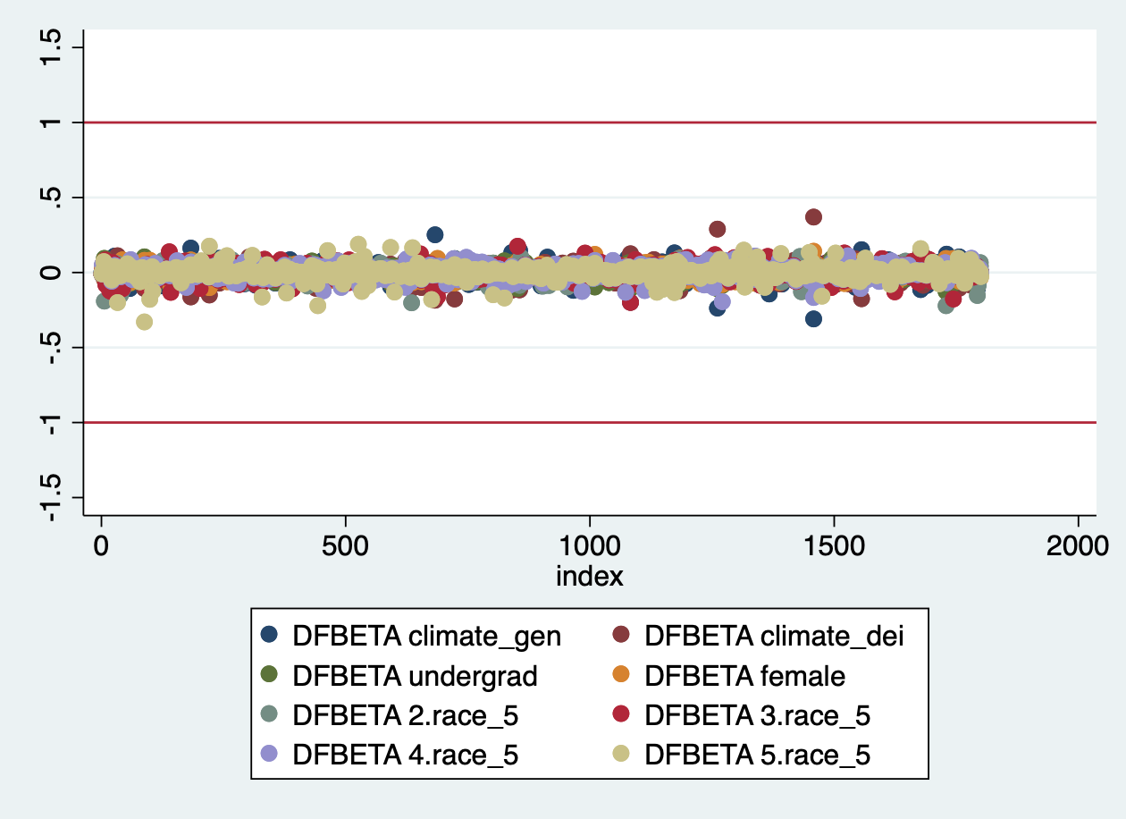
18.3 Joint Tests
Sometimes, you might want to carry out a joint test of coefficients. This is particularly important if you are concerned about bias within your model/a multicollinearity you are worried you can’t/don’t want to solve.
regress satisfaction climate_gen climate_dei undergrad female i.race_5
estimates store dei1
Source | SS df MS Number of obs = 1,434
-------------+---------------------------------- F(8, 1425) = 126.39
Model | 640.55287 8 80.0691087 Prob > F = 0.0000
Residual | 902.772793 1,425 .633524767 R-squared = 0.4150
-------------+---------------------------------- Adj R-squared = 0.4118
Total | 1543.32566 1,433 1.0769893 Root MSE = .79594
-------------------------------------------------------------------------------
satisfaction | Coefficient Std. err. t P>|t| [95% conf. interval]
--------------+----------------------------------------------------------------
climate_gen | .5605185 .03842 14.59 0.000 .4851528 .6358843
climate_dei | .297791 .0352098 8.46 0.000 .2287223 .3668597
undergrad | .0367544 .0439463 0.84 0.403 -.049452 .1229607
female | -.1016334 .0435345 -2.33 0.020 -.1870321 -.0162348
|
race_5 |
AAPI | -.0726621 .0588523 -1.23 0.217 -.1881086 .0427844
Black | -.5321254 .0692022 -7.69 0.000 -.6678745 -.3963762
Hispanic/L~o | -.1192444 .0608858 -1.96 0.050 -.2386798 .0001909
Other | -.124321 .0759098 -1.64 0.102 -.273228 .024586
|
_cons | .6662546 .1341078 4.97 0.000 .4031847 .9293245
-------------------------------------------------------------------------------test (climate_gen = 0) (climate_dei = 0) ( 1) climate_gen = 0
( 2) climate_dei = 0
F( 2, 1425) = 357.42
Prob > F = 0.0000The hypothesis test here is that these two coefficients TOGETHER have a value of 0. The fact that we have a p-value < 0.05 means we reject the hypothesis and find that AT LEAST ONE OF THESE VARIABLES HAS A RELATIONSHIP GREATER THAN 0.
BONUS
Though we don’t cover this in class, you can also use the ‘test’ command to
find out if two variables are equal to each other. This is especially useful
if your question is related to: whether theory 1 (var1) has a significiantly
different effect from theory 2 (var2).
For example: I’m interested in which of these (general climate / dei climate) has a greater effect on student satisfaction. I can use test to see if their coefficients are equal (if var1-var2 = 0),
test climate_gen = climate_dei ( 1) climate_gen - climate_dei = 0
F( 1, 1425) = 15.69
Prob > F = 0.0001You might think: how do I interpret this? The null hypothesis here is that the two coefficients are EQUAL to each other. Since p-value<0.5, we reject the null hypothesis, telling us the two variables are statistically different from each other. Given what our results shows us, we can then see that the difference is that general climate has a greater effect on satisfaction for students than dei climate.