3 Lab 1 (R)
3.1 Lab Goals & Instructions
- Review the basics of data cleaning
- Learn the importance of annotating code
- Start develop your own coding style
Instructions
- Download the data file (
SOC401_W21_Billionaires.rda) and R script (401-1-Lab1.R) from the links below. - Create a project following the instructions in 3.3 below
- Work through the R script, executing each line of code. This page contains the same material, with more explanation about the functions used.
- Read through the Importance of Annotation and Clean Code, and complete the short activity at the bottom of the page. Email the .R script file to me by class on Monday.
Jump Links to Functions in this Lab:
Global view of dataset
List of variable names
First 10 rows of data set or variable values
Missing observations
Descriptive statistics
Frequency tables
mutate
ifelse
Histogram with base R
Histogram with ggplot
Boxplot with ggplot
Bar plot with ggplot
select
filter
Save data files
3.3 Create a Project
In R, it is always best to work within what is called a “Project” when you are coding and analyzing data. Life can get messy and so can data analysis. Creating a project and a file structure is the equivalent of keeping a clean work space. You may not mind a messy desk, but a messy file structure will be a nightmare for your collaborators and increase your risk of making mistakes in your analysis. With quantitative data analysis, file management is crucial.
RStudio has created a wonderful project management tool for you. It’s an umbrella file that organizes all your scripts, folders, figures, and more. It also sets your working directory for you, which we will discuss more below.
For your first task, create a project in R for this class.
- Open RStudio.
- Click the “File” menu button, then “New Project.”
- Click “New Directory.”
- Click “New Project.”
- Type in the name of the directory to store your project, e.g. “401-1_Linear Regression.” Make sure you choose the parent folder on your computer where you want these files to be stored. Your project will live in new folder with the name you gave your directory. Your project and all your files will be stored there.
- Click the “Create Project” button.
Now let’s make sure you can open this project, create a file folder structure, and move your lab files for today into the appropriate spot.
- Exit RStudio
- Navigate to the folder where you created your directory. Double click on the
.Rprojfile you created.
- Open up a blank R script and use the following code to create a file structure.
dir.create("data_raw")
dir.create("data_work")
dir.create("fig_output")
dir.create("scripts")- Move
SOC401_W21_Billionaires.rdato yourdata_rawfolder. - Move
401-1-Lab1.Rto yourscriptsfolder.
For more information on best data management practices, and to see the source of some of the instructions above check out this R tutorial.
![]() Data Tip
Data Tip
Why do I need two separate folders for data?
You should aways store your original, raw data files in a place where they are in no danger of being saved over, altered, or lost. One great way of protecting your original data files is to create two folders for data: one folder for your raw files and one folder where you can saved cleaned datasets and subsets.
3.4 Data Cleaning
Ninety-five percent of the work of quantitative research is getting your data in shape to run your model. This tutorial assumes that you have R downloaded and are familiar with the basics of the language. If you are not, here are some resources to help you get started coding in R.
- R for Data Science. A great online book to help you learn R on your own.
- R Programming Tutorials on Youtube
- A quick tutorial for the Tidyverse. The tidyverse makes datacleaning in R a much simpler process.
- A great book on ggplot2. ggplot2 is the best package for making graphs in any software.
Northwestern’s Research Computing Services offers great trainings in a variety of software languages, including R, on a regular basis. Check them out and get on their email list.
Set up the environment
Before you get to work cleaning your data, you need to let the software know where to grab and save your files. This saves you from having to type in a long file path anytime you want to do something. If you are working in a project, you are good to go! Not sure if you are working in your project? If you look in the top right corner of your RStudio window, you should see the name of you project next to the project icon. If you see “None” or a different name, that means you need to open your project and start working from there!
If you are not working in a project, you should begin your file by setting your working directory. Your working directory is the folder on your computer where you want to store all your data and script files. Below you will see the path to my working directory. You should replace the filepath with the one you want to use.
# Set your working directory
setwd("~/Documents/Work & Research/Regression Labs")
Load your libraries
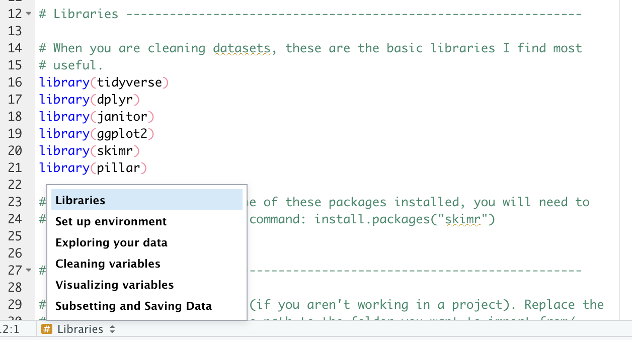
When you are cleaning datasets these are the basic packages that are useful. Make sure you load them before beginning work.
library(tidyverse)
library(dplyr)
library(janitor)
library(ggplot2)
library(skimr)
library(pillar)
Error in library(kableExtra): there is no package called 'kableExtra'Note: if you do not have one of these packages installed, you will need to first install it using the command: install.packages("skimr")
Load your data
Now that you’ve set your working directory, you can tell R to go grab your data and load it into your working environment.
Loading data that is in R’s data formats is easy. An R data file ends in .rda or .rData.
load("data_raw/SOC401_W21_Billionaires.rda")You can also load data in other formats. Here are a few common ones.
# Stata
read_dta("data_raw/SOC401_W21_Billionaires.dta")

# CSV
read.csv("data_raw/SOC401_W21_Billionaires.csv")
Check out this tutorial on how to load excel data:
https://www.datacamp.com/community/tutorials/r-tutorial-read-excel-into-r
At this point, it can also be helpful to rename your dataset to something short and easy to type. You are going to be typing it a lot in your R code.
mydata <- SOC401_W21_Billionaires # this saves the dataset as a new dataframe in our environment.Exploring your data
When you begin any new project, it is important to understand the condition of your variables. Here are a few important functions you need to begin that process.
![]() Data Tip
Data Tip
Remember if this script or any other uses a function that you are not familiar with, you can search for the function online or type ‘?’ and then the name of the function you want to look up in the console. For example, ‘?ifelse( )’ will pull up the documentation for that function.
Let’s start by taking a global look at your dataset.
There are countless ways to do this, but I am providing you with two helpful functions from two different packages.
Option 1 from the skimr library:
Note: The formatting of this web page is cutting off some columns in the table. I’m working on a fix but take a look at the results when you run it in your R script.
skim_without_charts(mydata)| Name | mydata |
| Number of rows | 2614 |
| Number of columns | 21 |
| _______________________ | |
| Column type frequency: | |
| character | 5 |
| numeric | 16 |
| ________________________ | |
| Group variables | None |
Variable type: character
| skim_variable | n_missing | complete_rate | min | max | empty | n_unique | whitespace |
|---|---|---|---|---|---|---|---|
| name | 0 | 1 | 5 | 45 | 0 | 2077 | 0 |
| companyname | 0 | 1 | 0 | 59 | 38 | 1578 | 0 |
| wealthhowfromemerging | 0 | 1 | 4 | 4 | 0 | 1 | 0 |
| wealthhowwasfounder | 0 | 1 | 4 | 4 | 0 | 1 | 0 |
| wealthhowwaspolitical | 0 | 1 | 4 | 4 | 0 | 1 | 0 |
Variable type: numeric
| skim_variable | n_missing | complete_rate | mean | sd | p0 | p25 | p50 | p75 | p100 |
|---|---|---|---|---|---|---|---|---|---|
| rank | 0 | 1.00 | 5.996700e+02 | 4.678900e+02 | 1 | 215.0 | 430 | 9.880e+02 | 1.565e+03 |
| year | 0 | 1.00 | 2.008410e+03 | 7.480000e+00 | 1996 | 2001.0 | 2014 | 2.014e+03 | 2.014e+03 |
| companyfounded | 0 | 1.00 | 1.924710e+03 | 2.437800e+02 | 0 | 1936.0 | 1963 | 1.985e+03 | 2.012e+03 |
| demographicsage | 0 | 1.00 | 5.334000e+01 | 2.533000e+01 | -42 | 47.0 | 59 | 7.000e+01 | 9.800e+01 |
| locationgdp | 0 | 1.00 | 1.769103e+12 | 3.547083e+12 | 0 | 0.0 | 0 | 7.250e+11 | 1.060e+13 |
| wealthworthinbillions | 0 | 1.00 | 3.530000e+00 | 5.090000e+00 | 1 | 1.4 | 2 | 3.500e+00 | 7.600e+01 |
| wealthhowinherited2 | 0 | 1.00 | 4.390000e+00 | 1.190000e+00 | 1 | 4.0 | 5 | 5.000e+00 | 6.000e+00 |
| wealthhowcategory2 | 1 | 1.00 | 4.660000e+00 | 1.650000e+00 | 1 | 3.0 | 5 | 6.000e+00 | 9.000e+00 |
| wealthtype2 | 22 | 0.99 | 3.060000e+00 | 1.200000e+00 | 1 | 2.0 | 3 | 4.000e+00 | 5.000e+00 |
| wealthhowindustry2 | 1 | 1.00 | 8.720000e+00 | 4.640000e+00 | 1 | 4.0 | 9 | 1.300e+01 | 1.900e+01 |
| locationregion2 | 0 | 1.00 | 4.240000e+00 | 1.720000e+00 | 1 | 3.0 | 4 | 6.000e+00 | 8.000e+00 |
| locationcountrycode2 | 0 | 1.00 | 4.567000e+01 | 2.417000e+01 | 1 | 23.0 | 48 | 7.100e+01 | 7.400e+01 |
| locationcitizenship2 | 0 | 1.00 | 4.676000e+01 | 2.386000e+01 | 1 | 23.0 | 53 | 7.100e+01 | 7.300e+01 |
| demographicsgender2 | 34 | 0.99 | 1.900000e+00 | 3.000000e-01 | 1 | 2.0 | 2 | 2.000e+00 | 3.000e+00 |
| companysector2 | 23 | 0.99 | 2.718500e+02 | 1.436600e+02 | 1 | 132.0 | 299 | 4.020e+02 | 5.200e+02 |
| companyrelationship2 | 46 | 0.98 | 4.527000e+01 | 1.827000e+01 | 1 | 32.0 | 32 | 6.600e+01 | 7.400e+01 |
The skim_without_charts() function does several great things. It includes the number of observations (rows) and variables (columnns), separates the variables by type (e.g., character vs. numeric), it has a nice compact presentation format, and includes all your basic descriptive statistics.
Option 2 from the pillar library:
glimpse(mydata)Rows: 2,614
Columns: 21
$ name <chr> "Bill Gates", "Bill Gates", "Bill Gates", "Warre…
$ rank <dbl> 1, 1, 1, 2, 2, 2, 3, 3, 3, 4, 4, 4, 5, 5, 5, 6, …
$ year <dbl> 1996, 2001, 2014, 1996, 2001, 2014, 1996, 2001, …
$ companyfounded <dbl> 1975, 1975, 1975, 1962, 1962, 1990, 1896, 1975, …
$ companyname <chr> "Microsoft", "Microsoft", "Microsoft", "Berkshir…
$ demographicsage <dbl> 40, 45, 58, 65, 70, 74, 0, 48, 77, 68, 56, 83, 7…
$ locationgdp <dbl> 8.10e+12, 1.06e+13, 0.00e+00, 8.10e+12, 1.06e+13…
$ wealthworthinbillions <dbl> 18.5, 58.7, 76.0, 15.0, 32.3, 72.0, 13.1, 30.4, …
$ wealthhowfromemerging <chr> "True", "True", "True", "True", "True", "True", …
$ wealthhowwasfounder <chr> "True", "True", "True", "True", "True", "True", …
$ wealthhowwaspolitical <chr> "True", "True", "True", "True", "True", "True", …
$ wealthhowinherited2 <dbl> 5, 5, 5, 5, 5, 5, 1, 5, 5, 5, 5, 5, 5, 5, 5, 4, …
$ wealthhowcategory2 <dbl> 4, 4, 4, 7, 7, 5, 4, 4, 5, 3, 4, 7, 3, 5, 4, 3, …
$ wealthtype2 <dbl> 2, 2, 2, 2, 2, 4, 3, 2, 2, 5, 2, 2, 5, 2, 2, 3, …
$ wealthhowindustry2 <dbl> 15, 15, 15, 3, 3, 7, 16, 15, 14, 13, 15, 3, 6, 1…
$ locationregion2 <dbl> 6, 6, 6, 6, 6, 4, 3, 6, 3, 2, 6, 6, 2, 3, 6, 2, …
$ locationcountrycode2 <dbl> 71, 71, 71, 71, 71, 47, 11, 71, 23, 30, 71, 71, …
$ locationcitizenship2 <dbl> 71, 71, 71, 71, 71, 39, 62, 71, 58, 25, 71, 71, …
$ demographicsgender2 <dbl> 2, 2, 2, 2, 2, 2, NA, 2, 2, 2, 2, 2, 2, 2, 2, 2,…
$ companysector2 <dbl> 5, 5, 5, 3, 3, 2, 379, 466, 13, 402, 10, 3, 66, …
$ companyrelationship2 <dbl> 32, 32, 32, 32, 32, 32, NA, 32, 32, 44, 32, 32, …The glimpse function is not as compact as skim, but it also includes the number of observations and variable, the class of each variable, and unlike skim it shows the first several observations for each variable. This can be helpful for seeing the structure of the values for each variable.
You can also get a list of all the variable names in your data set
names(mydata) [1] "name" "rank" "year"
[4] "companyfounded" "companyname" "demographicsage"
[7] "locationgdp" "wealthworthinbillions" "wealthhowfromemerging"
[10] "wealthhowwasfounder" "wealthhowwaspolitical" "wealthhowinherited2"
[13] "wealthhowcategory2" "wealthtype2" "wealthhowindustry2"
[16] "locationregion2" "locationcountrycode2" "locationcitizenship2"
[19] "demographicsgender2" "companysector2" "companyrelationship2" View the first 10 rows of your data set.
head(mydata)# A tibble: 6 × 21
name rank year companyfounded companyname demographicsage locationgdp
<chr> <dbl> <dbl> <dbl> <chr> <dbl> <dbl>
1 Bill Gates 1 1996 1975 Microsoft 40 8.1 e12
2 Bill Gates 1 2001 1975 Microsoft 45 1.06e13
3 Bill Gates 1 2014 1975 Microsoft 58 0
4 Warren Buf… 2 1996 1962 Berkshire … 65 8.1 e12
5 Warren Buf… 2 2001 1962 Berkshire … 70 1.06e13
6 Carlos Sli… 2 2014 1990 Telmex 74 0
# … with 14 more variables: wealthworthinbillions <dbl>,
# wealthhowfromemerging <chr>, wealthhowwasfounder <chr>,
# wealthhowwaspolitical <chr>, wealthhowinherited2 <dbl>,
# wealthhowcategory2 <dbl>, wealthtype2 <dbl>, wealthhowindustry2 <dbl>,
# locationregion2 <dbl>, locationcountrycode2 <dbl>,
# locationcitizenship2 <dbl>, demographicsgender2 <dbl>,
# companysector2 <dbl>, companyrelationship2 <dbl>View the first 10 observations of a specific variable
head(mydata$name)[1] "Bill Gates" "Bill Gates" "Bill Gates" "Warren Buffett"
[5] "Warren Buffett" "Carlos Slim Helu"Look at missing observations in your dataset
To apply this to your data set, just change mydata to the name of whatever dataset you are using. Everything else can stay the same.
sapply(mydata, function(x) sum(is.na(x))) name rank year
0 0 0
companyfounded companyname demographicsage
0 0 0
locationgdp wealthworthinbillions wealthhowfromemerging
0 0 0
wealthhowwasfounder wealthhowwaspolitical wealthhowinherited2
0 0 0
wealthhowcategory2 wealthtype2 wealthhowindustry2
1 22 1
locationregion2 locationcountrycode2 locationcitizenship2
0 0 0
demographicsgender2 companysector2 companyrelationship2
34 23 46 You can also pull up descriptive statistics for your entire data set using the summary function.
summary(mydata) name rank year companyfounded
Length:2614 Min. : 1.0 Min. :1996 Min. : 0
Class :character 1st Qu.: 215.0 1st Qu.:2001 1st Qu.:1936
Mode :character Median : 430.0 Median :2014 Median :1963
Mean : 599.7 Mean :2008 Mean :1925
3rd Qu.: 988.0 3rd Qu.:2014 3rd Qu.:1985
Max. :1565.0 Max. :2014 Max. :2012
companyname demographicsage locationgdp wealthworthinbillions
Length:2614 Min. :-42.00 Min. :0.000e+00 Min. : 1.000
Class :character 1st Qu.: 47.00 1st Qu.:0.000e+00 1st Qu.: 1.400
Mode :character Median : 59.00 Median :0.000e+00 Median : 2.000
Mean : 53.34 Mean :1.769e+12 Mean : 3.532
3rd Qu.: 70.00 3rd Qu.:7.250e+11 3rd Qu.: 3.500
Max. : 98.00 Max. :1.060e+13 Max. :76.000
wealthhowfromemerging wealthhowwasfounder wealthhowwaspolitical
Length:2614 Length:2614 Length:2614
Class :character Class :character Class :character
Mode :character Mode :character Mode :character
wealthhowinherited2 wealthhowcategory2 wealthtype2 wealthhowindustry2
Min. :1.000 Min. :1.000 Min. :1.000 Min. : 1.000
1st Qu.:4.000 1st Qu.:3.000 1st Qu.:2.000 1st Qu.: 4.000
Median :5.000 Median :5.000 Median :3.000 Median : 9.000
Mean :4.386 Mean :4.662 Mean :3.055 Mean : 8.715
3rd Qu.:5.000 3rd Qu.:6.000 3rd Qu.:4.000 3rd Qu.:13.000
Max. :6.000 Max. :9.000 Max. :5.000 Max. :19.000
NA's :1 NA's :22 NA's :1
locationregion2 locationcountrycode2 locationcitizenship2 demographicsgender2
Min. :1.000 Min. : 1.00 Min. : 1.00 Min. :1.000
1st Qu.:3.000 1st Qu.:23.00 1st Qu.:23.00 1st Qu.:2.000
Median :4.000 Median :48.00 Median :53.00 Median :2.000
Mean :4.236 Mean :45.67 Mean :46.76 Mean :1.905
3rd Qu.:6.000 3rd Qu.:71.00 3rd Qu.:71.00 3rd Qu.:2.000
Max. :8.000 Max. :74.00 Max. :73.00 Max. :3.000
NA's :34
companysector2 companyrelationship2
Min. : 1.0 Min. : 1.00
1st Qu.:132.0 1st Qu.:32.00
Median :299.0 Median :32.00
Mean :271.9 Mean :45.27
3rd Qu.:402.0 3rd Qu.:66.00
Max. :520.0 Max. :74.00
NA's :23 NA's :46 You can use the same function to look at a specific variable.
summary(mydata$wealthworthinbillions) Min. 1st Qu. Median Mean 3rd Qu. Max.
1.000 1.400 2.000 3.532 3.500 76.000 If you want to look at individual descriptive statistics, you can use the following functions to get the mean, range, or standard deviation of variables. These functions can be helpful checks as you work on cleaning a dataset.
mean(mydata$demographicsage)[1] 53.34124range(mydata$demographicsage) #hmm...notice anything odd about this range?[1] -42 98sd(mydata$demographicsage)[1] 25.33332You can also produce a frequency table for a specific variable.
This function makes use of pipes (%>%) and tidyverse functions. It starts with a dataset and pipes that data through various commands. In this command, we tell R to group the data by year and then count the number of observations for each unique year in the dataset.
mydata %>%
  group_by(year) %>%
  count()
# A tibble: 3 × 2
# Groups: year [3]
year n
<dbl> <int>
1 1996 423
2 2001 538
3 2014 1653If you want to add percentages to the table, you can add another column to the table and calculate the percentage. We also make use of the round() function to limit the values to two decimals.
mydata %>%
  group_by(year) %>%
  count() %>%
  mutate(percent = round(n / nrow(mydata) * 100, 2))
# A tibble: 3 × 3
# Groups: year [3]
year n percent
<dbl> <int> <dbl>
1 1996 423 16.2
2 2001 538 20.6
3 2014 1653 63.2Cleaning variables
In the previous section, we learn the code to check the state of a variable when we first open the dataset. Most of the time, you’re likely to find that the variable isn’t ideal to work with. It is important to use this commands to make a variable ready for your use.
Let’s take a closer look at the variable for gender:
mydata %>%
  group_by(demographicsgender2) %>%
  count()
# A tibble: 4 × 2
# Groups: demographicsgender2 [4]
demographicsgender2 n
<dbl> <int>
1 1 249
2 2 2328
3 3 3
4 NA 34With this code, we use a pipe (%>%) to create a frequency table to see what the values and frequencies look like. I notice a few things you will want to change about that variable:
- The variable name is tedious to type
- We want this to be a dummy variable where 1 is female and 0 is not female (in this binary, male).
- We have three married couples in our data set coded as 3
Let’s create a new variable with a better name and recode it how you’d like it.
Here you will recode the variable using the mutate() function and the ifelse() function, which are helpful for recoding based on previous variable.
If you want to label the 3 married couples as 0, aka not female…
# Recode the variable
mydata <- mydata %>%
  mutate(female = ifelse(demographicsgender2 == 1, 1, 0))

# Check the new variable using a frequency table.
mydata %>%
  group_by(female) %>%
  count()
# A tibble: 3 × 2
# Groups: female [3]
female n
<dbl> <int>
1 0 2331
2 1 249
3 NA 34For this recoding we used two new functions.
mutate() to create new variables
mutate() is a function found in the tidyverse to create a new variable. You simple put the name of the new variable we want to use, a single equals sign, and whatever code will create the variable we want. In this case you’re saying create a new variable named female and set it equal to 1 if the previous variable, demographicsgender2, is equal to 1 and set it equal to 0 if it’s any other value. R maintains the missing variables in this case.
Note: In R when you are creating something new, as inside of the mutate statement, you use a single equals sign. Your new variable female should equal what follows. When you’re writing a test statement referring to something that already exists, you use double equals sign (==). For example, in the ifelse function you use two equals sign because you’re looking at the data where demographicsgender2 is in existing data equal to 1.
ifelse() to write conditional statements
ifelse() is an incredibly helpful function to recode one variable based on its existing values or the values of another variable. The function requires you to specify some type of condition. In this case you’re saying make this change if demographicsgender2 is equal to 1. If it is equal to one, you tell R what you want to do after the comma– set the value of your new variable equal to one. After the next comma, you tell R if else (meaning if demographicsgender2 is any other value) set the value of our new variable equal to 1.
ifelse(test statement, value if test is true, value if test is false)
You can also nest ifelse statements. This is helpful when you have more two values you are recoding. For example, if you want to label the three married couples as NA, so 1 = female, 0 = male you can nest ifelse statements.
# Recode
mydata <- mydata %>%
  mutate(female = ifelse(demographicsgender2 == 1, 1, # if gender = 1, recode 1
                         ifelse(demographicsgender2 == 2, 0, NA))) # if gender = 2, recode 0, ifelse value should be missing.

# Check the new variable
mydata %>%
  group_by(female) %>%
  count()
# A tibble: 3 × 2
# Groups: female [3]
female n
<dbl> <int>
1 0 2328
2 1 249
3 NA 37Note: by running these two chunks of code back to back, I wrote over my first attempt at creating a new dummy variable ‘female.’ If I want to use the second one that’s fine, but there’s no going back once you overwrite something, so be careful with your code.
Now let’s try another example, looking at the variable for age:
mydata %>%
  group_by(demographicsage) %>%
  count()
# A tibble: 76 × 2
# Groups: demographicsage [76]
demographicsage n
<dbl> <int>
1 -42 1
2 -7 1
3 0 383
4 12 1
5 21 1
6 24 2
7 28 2
8 29 4
9 30 4
10 31 5
# … with 66 more rowsThe major concern is that there are some numbers that seem unreasonable. Age is not negative, and 0 is an unlikely age for a person in a billionaire dataset. Let’s recode those variables to missing (NA) for now. Again, you’ll use mutate() and ifelse(), and you will name the variable something easier to work with. Here if the test statement is false (aka if demographicsage is greater than 0) the value should just transfer over from demographicsage.
# Recode the variable
mydata <- mydata %>%
  mutate(age = ifelse(demographicsage <= 0, NA, demographicsage))

# Check the new variable
mydata %>%
  group_by(age) %>%
  count()
# A tibble: 74 × 2
# Groups: age [74]
age n
<dbl> <int>
1 12 1
2 21 1
3 24 2
4 28 2
5 29 4
6 30 4
7 31 5
8 32 4
9 33 8
10 34 6
# … with 64 more rows![]() Data Tip
Data Tip
Why create a new variable when recoding?
If you have a sharp eye, you’ll notice that we created a new variable rather than changing the name of our original variable and recoding it. Data cleaning is an iterative process. You may make mistakes (you will probably make mistakes) or you may change your mind about how to recode a variable. In each case, having the original variable on hand is always helpful. To preserve your original variable, you create a new variable rather than writing over the old one.
Vizualizing variables
Continuous Variables
While frequency tables and descriptive statistics are helpful, visualizing variables can be helpful to get a look at the shape of our data. For continuous variables or discrete variables with a wide range of values histograms or box plots the go to.
There are two main ways to create graphs in R, base R plots and ggplot2. ggplot2 has far more flexibility, so we will focus on that package primarily. However, when you are moving fast it can sometimes be helpful to throw up a quick histogram in base R.
hist() to create a histogram in base R
The code for creating a histogram using base R is simple, but you don’t have as much flexibility to change aspects of the plot if you want to use it in presentations or papers.
hist(mydata$age)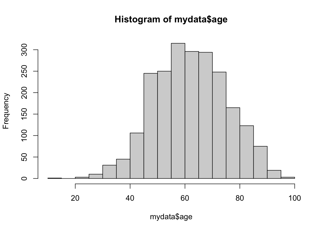
If you want to change the number of bins (i.e. bars), you add a breaks argument to the function.
hist(mydata$age, breaks = 10)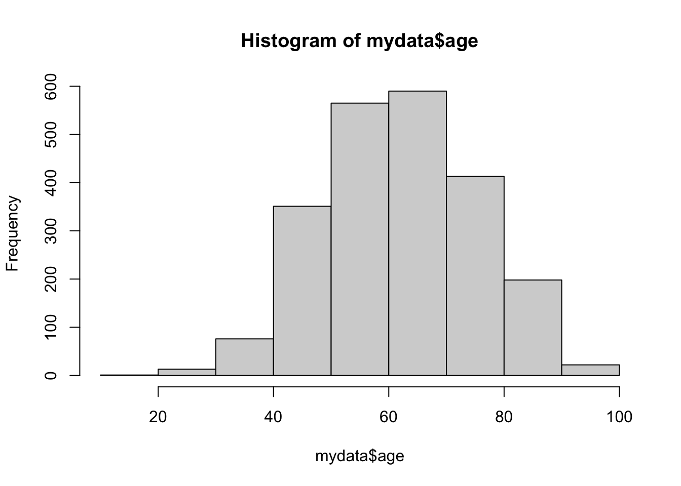
Histograms in ggplot2
As I’ve mentioned, ggplot2 has a massive amount of flexibility and a unique grammar to building plots. It is the go-to package to produce quality plots and graphics, but is a lot to learn to use it with ease. If you are interested I recommend taking a ggplot2 workshop or working through the ggplot2 book listed in resources at the beginning of this lab. For now, let’s build a simple histogram using the ggplot() function.
# Creatign the plot
ggplot(data = mydata, aes(x = age)) + #specifying dataset and your variable
  geom_histogram(color = "white") + #changing the outline of the bars to white
  theme_classic() # applying a built-in theme to the graph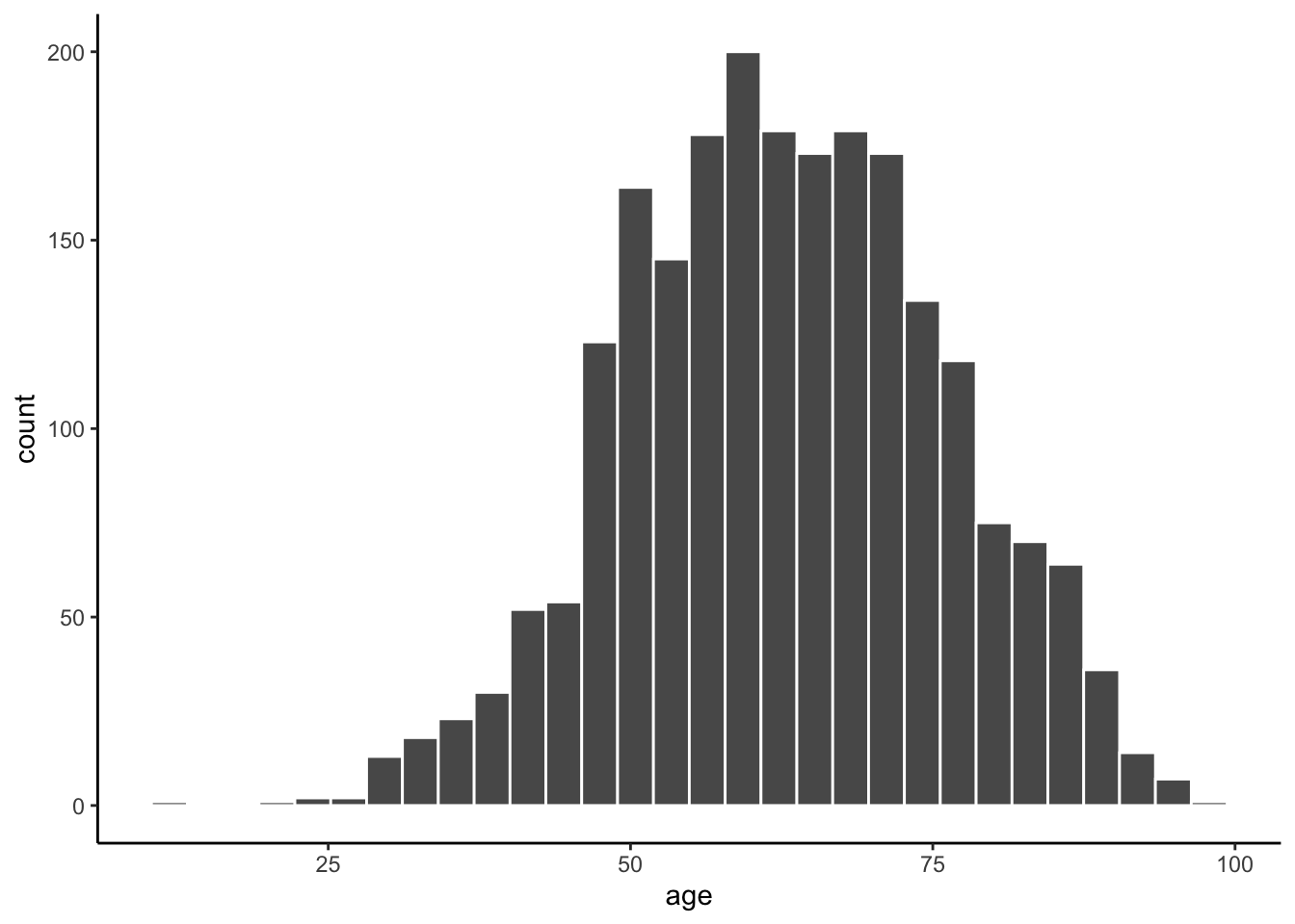
Let’s try changing the number of bins.
ggplot(data = mydata, aes(x = age)) +
  geom_histogram(color = "white", bins = 10) +
  theme_classic()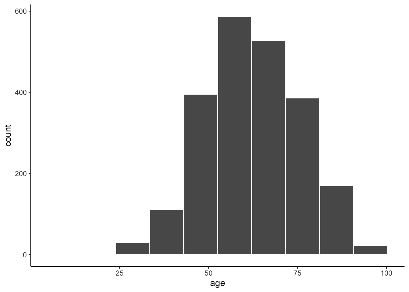
Box plots with ggplot()
Let’s try making a boxplot of age.
ggplot(data = mydata, aes(y = age)) + # Calling the same data, but switched to y axis so the boxplot would be vertical
  geom_boxplot() + # calling the boxplot geom
  theme_bw() # trying a different theme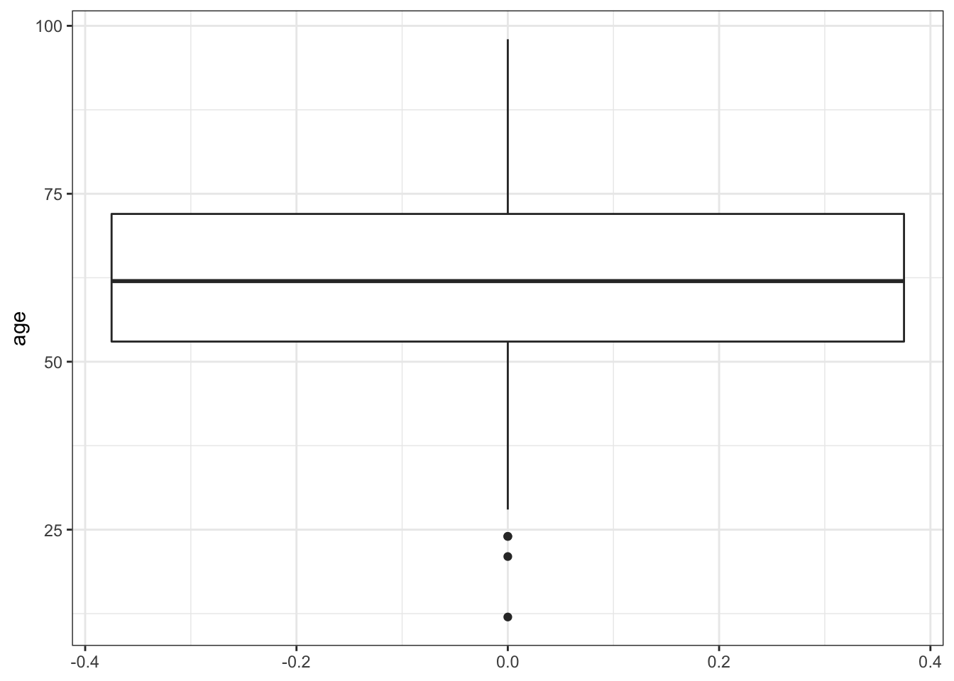
Let’s try making a boxplot of age by gender.
ggplot(data = mydata, aes(y = age, x = female, group = female)) +
  # adding x to label the x axis, and grouping by the same variable to create two box plots
  geom_boxplot() + # same geom
  theme_bw() #same theme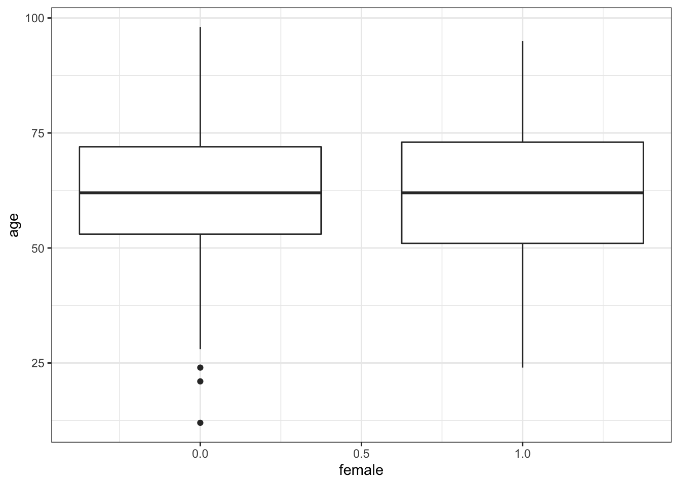
3.4.0.1 Categorical Variables
Again frequency tables are great, but sometimes a visualization of a categorical data can better communicate patterns.
Bar plots with ggplot()
Let’s try making a bar plot of gender. Note I have to turn female into a factor. This doesn’t permanently transform the variable. It just temporarily transforms the variable for this plot.
ggplot(data = mydata, aes(x = as.factor(female))) +
  geom_bar() +
  theme_minimal()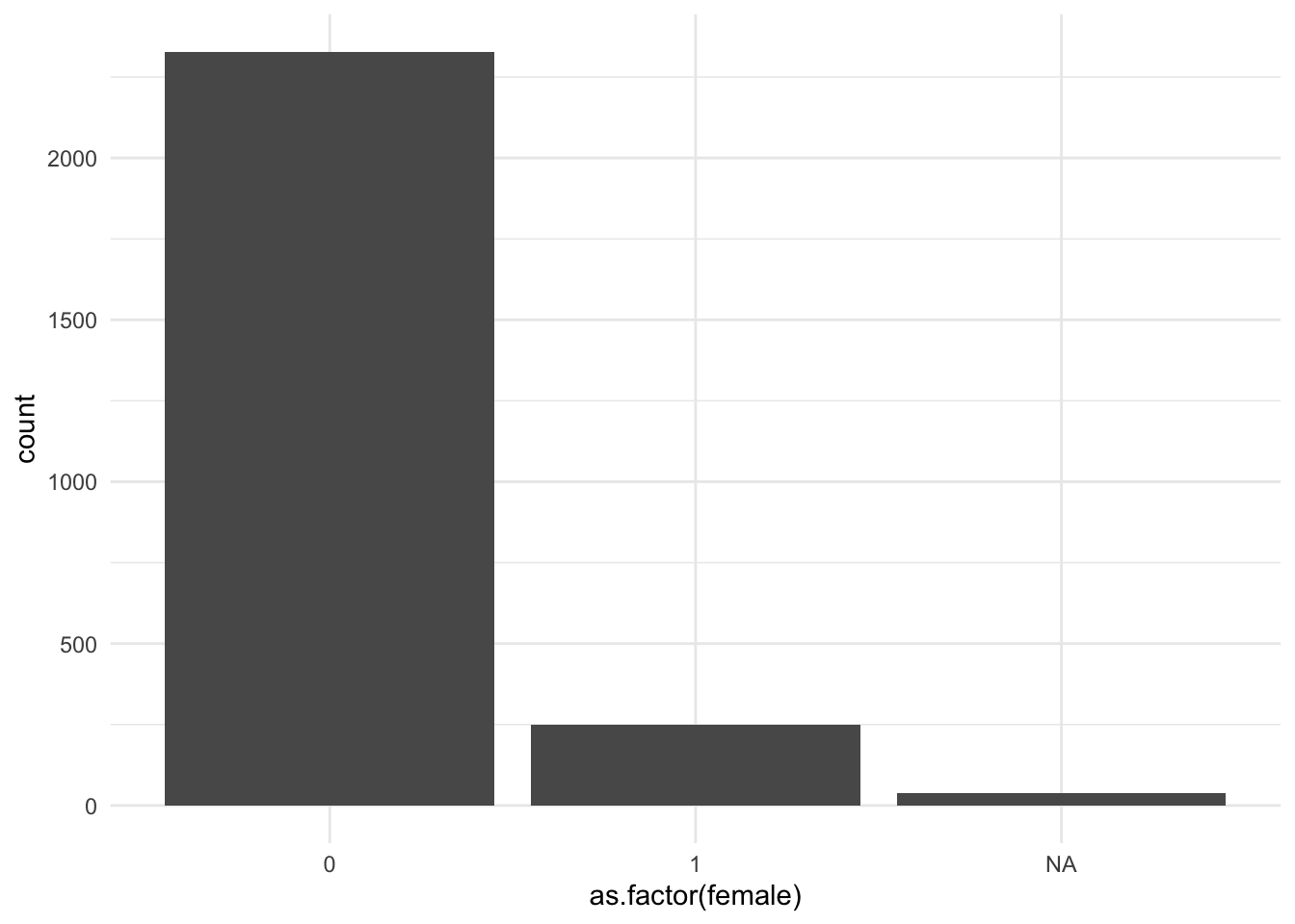
If I want to remove the NA column, I can also filter the data within the ggplot function. I’m also going to clean up the axis labels, add a title, and change the width of the bars.
ggplot(data = mydata %>% drop_na(female), aes(x = as.factor(female))) +
  geom_bar(width = .5) +
  labs(
    x = "Gender",
    y = "Count",
    title = "Bar plot of gender"
  ) +
  theme_minimal()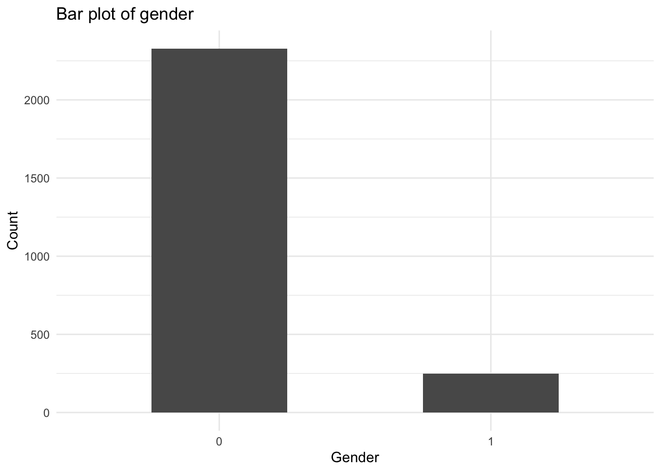
Another advantage of ggplot is that the code to save is much easier than base R plots. This code will save the last ggplot that you created. I encourage you to look up other examples of ggsave to learn different ways you can save plots as objects, specify height and width, and more.
ggsave("figs_output/barplot-example.png")Subsetting and saving data
Sometimes you’ll be working with a huge dataset, and it is easier and cleaner save a portion of observations and/or variables in a new dataset. This is called a subset.
select() to subset your data to specific variables
Let’s say you only want to keep the following three variables: year and the two variables you just created: age and female. You can easily subset the data using the select() function in tidyverse. In the select function you simply list the variables you want to keep. You can also specify specific variables to drop by putting them in the list with a minus sign in front (example: -year, -age, -female)
mysubset <- mydata %>% # note I'm saving this as a new dataframe with a new name
  select(year, age, female)

glimpse(mysubset) # you should always check your data when you make a major change like adding or removing variables.
Rows: 2,614
Columns: 3
$ year <dbl> 1996, 2001, 2014, 1996, 2001, 2014, 1996, 2001, 2014, 1996, 200…
$ age <dbl> 40, 45, 58, 65, 70, 74, NA, 48, 77, 68, 56, 83, 71, NA, 69, NA,…
$ female <dbl> 0, 0, 0, 0, 0, 0, NA, 0, 0, 0, 0, 0, 0, 0, 0, 0, 0, 0, 0, 0, 0,…filter() to subset your data to specific observations
But what if you wanted to subset the data to only billionaires 30 or older? For this task, you can use the filter() function. Filter acts exactly like the name implies. Use a conditional statement to specify what observations you want to keep or remove from your dataset.
# Filtering data to only billionaires over 30
mysubset2 <- mydata %>%
  filter(age >= 30)

range(mysubset2$age) # Another check to see our code worked how we wanted it!
[1] 30 98Saving your subset
Now that you have your subset, you’ll want to save it. Saving in R’s data, format is simple.
# Saving as r data format (.rda or .rData - both are the same).
save(mysubset, file = "data_work/mysubset.rda") # note I'm saving this in my working data folder
There are extra steps to save it other formats. .CSV files, are one of the most common formats you’ll receive and save data in outside of R.
write_csv(mysubset, file = "data_work/mysubset.csv")Remember, every time you run these command it writes over your previous save. So be careful about version control and ALWAYS maintain the raw data file in a separate location.
3.5 The Importance of Annotation and Clean Code
A script is not just a functional document where you conduct your analysis. It is also an important record of your analysis. When you read back through your script files you should be able to understand what each step of code is doing and why. Well-written code scripts:
- Have a header with your name and a title or a short description of what the script contains (e.g., “Cleaning data for regression analysis on billionaires”)
- Document the analytic decisions made about cleaning and analysis
- Can be run from start to finish without errors
You may think that you will remember what you were thinking when you wrote a script, but sometimes you’ll have to step away from an analysis for weeks or months. When you come back to it, your notes will remind you exactly why you coded things the way you did. Your code scripts will also be read by other people. It may be collaborators, advisers, or colleagues who agree to quality check your code to look for errors. It is also more and more common for journals to ask scholars to post their coding files so that other people can replicate your analysis.
How to make notes in your script
The main way to make a note in an R script is to use the #. You can put the # at the beginning of the line or after a piece of code. Whatever you type after the # will be colored green to indicate notation text that will not be run as code.
Let’s return to our code to filter our data. In this code I note above the command what it is about to do. In the second command, I include a note one the same line to remind myself that I want to check to make sure the code I ran worked correctly.
# Filtering data to only billionaires over 30
mysubset2 <- mydata %>%
  filter(age >= 30)

range(mysubset2$age) # Another check to see our code worked how we wanted it!
There’s one trick that can be helpful when writing notes in R script. Say you have a note that will take multiple lines. For example, you may want to document the source of the data you are using. If you put a single quotation mark after the hashtag (#'), R will automatically make the next line a comment when you press enter. It will work in regular .R scripts, but will not work in .Rmd files. Try it out!
#' This is a comment. When I press enter...
#' The next line will be a comment too.
#'
Finally, sometimes you may want to “comment out” a couple lines of code, either temporarily while you are coding or because you want to keep a record of code you don’t need to run again. R has a handy shortcut to let you turn a chunk of codes into comments and turn a chunk of comments into code. You do this by highlighting the chunk you want to comment in or out and typing Cmnd + Shift + C. For example, in the following code, I want to remove the line of code that adds a title to my ggplot. I may want to add it back in later, so rather than removing the line of code, I just commented it out. The grammar of tidyverse and ggplot2, with their pipes and plus signs, make it easy to comment out a specific type of code.
ggplot(data = mydata, aes(y = age, x = female, group = female)) +
  geom_boxplot() +
  # labs(
  #   title = "Boxplot of age by gender"
  # ) +
  theme_bw()
Tips for Neat Code
Notes are a huge part of making your code readable to yourself and others. However, writing neat code is also an enormous gift you can give to yourself, to the TA grading your scripts, and anyone else trying to make sense of your code. Here are my top tips for writing neat code in R:
- Split long functions and commands across multiple lines
- Leave spaces around equals signs and other operators
- Create headers and sections in your code
- Create clear names for your variables, data frames, and objects
Split long functions and commands across multiple lines
Nothing, I repeat, nothing makes code harder to read than shoving it all into one long line. R doesn’t care how many lines you split code across. It will run a function until it gets to the last closed parentheses. Splitting code across multiple lines makes it easier for you to see and edit your code. It makes it way more legible to others reading your code. Look at the difference between these two pairs of commands from earlier in this lab.
# Creating a frequency table with percentages
mydata %>% group_by(year) %>% count() %>% mutate(percent = round(n / nrow(mydata) * 100, 2))

# Creating a boxplot with a title
ggplot(data = mydata, aes(y = age, x = female, group = female)) + geom_boxplot() + labs(title = "Boxplot of age by gender") + theme_bw()
These lines of code will run just fine, but they are difficult for your eye to parse when squished together. Let your code breathe! Notice how in the clean version of this code below, I even split the labs() function across three lines. This may not matter as much here, but if I add an x axis label, y axis label, subtitle, and caption, I would put each on its own line for ease of reading and editing.
mydata %>%
  group_by(year) %>%
  count() %>%
  mutate(percent = round(n / nrow(mydata) * 100, 2))

ggplot(data = mydata, aes(y = age, x = female, group = female)) +
  geom_boxplot() +
  # labs(
  #   title = "Boxplot of age by gender"
  # ) +
  theme_bw()
As a rule, don’t let any line get past about 80 characters. RStudio includes a vertical line at about this point. I recommend that you don’t write past it in your code scripts. It will help you and the reader avoid the annoying horizontal scroll bar.
Leave spaces around operators
This is another tip to let your code breathe! When coding it is best practice to put a space after any comma or logical operator. Take the line of code below:
mutate(percent=round(n/nrow(mydata)*100,2))It works, but it’s cluttered and that makes it difficult to read. Take a look at this line in a cleaner format:
mutate(percent = round(n / nrow(mydata) * 100, 2))Notice how I’ve added a space on both sides of the =, the /, and the *. This makes it easier to understand and edit your code.
Create headers and sections in your code
You wouldn’t write a paper without any titles or sections, so don’t write your code without titles or sections! Take a look back at the R script for this lab. Notice how I put a section header for setting up your environment, exploring your data, cleaning your data, and so on. Hopefully this made it easier for you to work through the script.
You can create headers with comments, but you can also use a shortcut built into R. If you go to Code -> Insert Section or Ctrl+Shift+R (Cmd+Shift+R on the Mac) this will insert a header and create a code section. Any comment line which includes at least four trailing dashes (-), equal signs (=), or pound signs (#) automatically creates a code section.
 # Section One ---------------------------------

 # Section Two =================================

 ### Section Three #############################
You can collapse and expand code sections or use a drop down menu to jump to a code section. Trust me when I say cleaning scripts can get long, and these section headers can be a huge time-saver.
Create clear names for your variables, data frames, and objects
Everyone has their own preferred naming system for variables, data frames, and other R objects. The golden rule for naming is consistency. For example, if I recode variables I will often add _rc to the end for recode (e.g., age and age_rc). Other tips:
- Make your names explicit, but brief (e.g.,
table_1,table_2) - Don’t include spaces in your file names, it makes file paths difficult
3.6 Activity
For this class, we expect you to write legible, clean code. To kick start this process, I want you to begin develop your own coding style. By class on Monday, email me (rosewerth@u.northwestern.edu) a script file for a hypothetical data cleaning script. The script should include:
- A script header with your name, the date you created the script, and a short description of what the script contains
- Two section headers
- A note telling me what you find easy about coding in R and what you find difficult about coding in R.
This should be your template for writing clean scripts for the rest of the quarter. Your template can evolve, but I expect all your scripts moving forward to contain title and section headers and clear annotation for each step in your code.