15 Lab 7 (R)
15.1 Lab Goals & Instructions
Goals
- Use robust standard errors to address heteroskedasticity in your models
- Check the VIF for your model to detect multicollinearity
- Review interpretation of log transformed variables
Instructions
- Download the data and the script file from the lab files below.
- Run through the script file and reference the explanations on this page if you get stuck.
- No challenge activity!
Libraries
# Load libraries
library(tidyverse)
library(ggplot2)
library(ggeffects)
library(car)
library(moments)
# install.packages("sandwich")
# install.packages("lmtest")
library(sandwich)
library(lmtest)
15.1.0.1 Data
We’re going to use two datasets in this lab. One advantage of coding in R is that we can load multiple datasets at once. So let’s load our two dataframes for today’s lab:
# Load UM DEI Survey Data
load("data_raw/UM_DEIStudentSurvey.rda")
df_umdei <- UM_DEIStudentSurvey #rename for ease

# Load WHO Life Expectancy Data
load("data_raw/who_life_expectancy_2010.rda")
df_who <- who_life_expectancy_2010
Jump Links to Commands in this Lab:
15.2 Robust Standard Errors
Heteroskedasticity is a complicated word with a simple solution:
Robust Standard Errors!
Remember that heteroskedascity occurs when our constant variance is violated. Though it doesn’t bias our coefficients, it does affect our t-statistics and standard errors. That means something could appear significant when it is not.
To address this, we essentially recalculate our standard errors after we
run our model. Then we interpret the results with the new standard errors.
We will use the function coeftest() from the “lmtest” package and the function vcovHC() from the "sandwich" package to do this.
STEP 1: Regression without robust standard errors
fit1 <- lm(satisfaction ~ climate_gen + climate_dei + instcom + undergrad +
                 female + race_5, data = df_umdei)
summary(fit1)
Call:
lm(formula = satisfaction ~ climate_gen + climate_dei + instcom +
    undergrad + female + race_5, data = df_umdei)

Residuals:
    Min      1Q  Median      3Q     Max
-3.5666 -0.4443  0.0807  0.5136  2.2515

Coefficients:
                      Estimate Std. Error t value Pr(>|t|)
(Intercept)            0.39065    0.13777   2.836 0.004640 **
climate_gen            0.52362    0.03776  13.867  < 2e-16 ***
climate_dei            0.13314    0.03899   3.415 0.000656 ***
instcom                0.29014    0.03297   8.800  < 2e-16 ***
undergrad             -0.01509    0.04307  -0.350 0.726112
female                -0.06553    0.04268  -1.535 0.124922
race_5Black           -0.37383    0.07677  -4.869 1.25e-06 ***
race_5Hispanic/Latino -0.05868    0.06899  -0.851 0.395129
race_5Other           -0.06355    0.08168  -0.778 0.436657
race_5White            0.05499    0.05727   0.960 0.337081
---
Signif. codes:  0 '***' 0.001 '**' 0.01 '*' 0.05 '.' 0.1 ' ' 1

Residual standard error: 0.7729 on 1418 degrees of freedom
  (372 observations deleted due to missingness)
Multiple R-squared:  0.4459,    Adjusted R-squared:  0.4424
F-statistic: 126.8 on 9 and 1418 DF,  p-value: < 2.2e-16
STEP 2: Check for heteroskedasticity First, look at the Residuals vs Fitted Values Plot:
plot(fit1, which = 1) 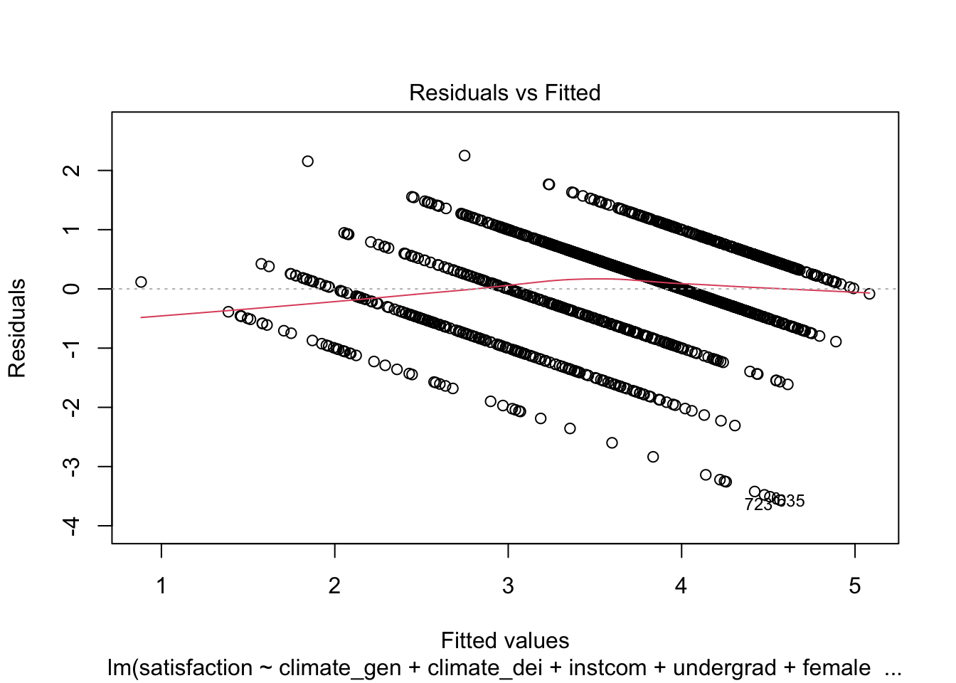
And the Standardized Residuals vs Predicted (Fitted) Values Plot
plot(fit1, which = 3) 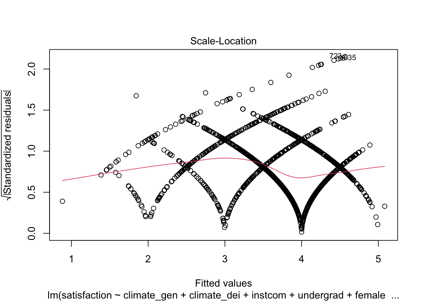
We can see that there is a pattern to the residuals and the standardized residuals plot does not have a flat horizontal line. Note: The residuals appear in lines because our outcome is technically categorical and we are treating it as if it were continuous.
STEP 3: Calculate robust standard errors
In R we use the functions coeftest() and vcovHC() to recalculate our results with robust standard errors. They are from the lmtest and sandwich packages. Here we are telling R to use type “HC1,” aka heteroskedasticity consistent, for our standard errors.
fit1_robust <- coeftest(fit1, vcov = vcovHC(fit1, type="HC1"))
fit1_robust
t test of coefficients:

                       Estimate Std. Error t value  Pr(>|t|)
(Intercept)            0.390650   0.128862  3.0315  0.002477 **
climate_gen            0.523621   0.043684 11.9865 < 2.2e-16 ***
climate_dei            0.133140   0.043780  3.0411  0.002400 **
instcom                0.290138   0.035738  8.1184 1.016e-15 ***
undergrad             -0.015091   0.042187 -0.3577  0.720611
female                -0.065531   0.041780 -1.5685  0.116992
race_5Black           -0.373835   0.074971 -4.9864 6.912e-07 ***
race_5Hispanic/Latino -0.058685   0.066538 -0.8820  0.377942
race_5Other           -0.063553   0.087700 -0.7247  0.468779
race_5White            0.054990   0.054268  1.0133  0.311083
---
Signif. codes:  0 '***' 0.001 '**' 0.01 '*' 0.05 '.' 0.1 ' ' 1
QUESTION: What changes? Based on these changes, how serious was heteroskedascity in this model?
Adding the robust standard errors doesn’t change that much in the model. You will see that the coefficients do not change, but the standard errors do. The changed standard errors then affect the t scores and p-values.
How bad does heteroskedasticity need to be to use robust standard errors?
The rule of thumb is that robust standard errors are the best almost all the time. Unless you see near perfect variance around 0 when you plot your residuals, it is always best to use robust standard errors.
!! Better safe than sorry!!
15.3 Detecting Multicollinearity
Multicollinearity occurs when some of your independent variables are too closely correlated with one another. When this happens, the model can’t separate the effects of each variable because they always vary together.
Checking for multicollinearity is a fairly straightforward process. What we do is check the VIF of our model after we run a regression. When a VIF is greater than 10, that is an indication that there is multicollinearity.
Example 1
Once you’ve run a regression, you can look at the VIF by using the vif() command from the car library. Let’s do it on our first regression.
vif(fit1) GVIF Df GVIF^(1/(2*Df))
climate_gen 1.818375 1 1.348471
climate_dei 2.408626 1 1.551975
instcom 1.879929 1 1.371105
undergrad 1.085469 1 1.041858
female 1.083664 1 1.040992
race_5 1.144954 4 1.017065What we find here is that our model has very little multicollinearity because everything in our model has a vif (variance inflation factor) that is below 10.
Example 2
Let’s take a look at one example where you might see higher vif.
fit2 <- lm(satisfaction ~ climate_gen + climate_dei + instcom + I(instcom^2) +
             undergrad + female + race_5, data = df_umdei)

vif(fit2)
GVIF Df GVIF^(1/(2*Df))
climate_gen 1.896119 1 1.376996
climate_dei 2.411104 1 1.552773
instcom 37.217078 1 6.100580
I(instcom^2) 35.188404 1 5.931981
undergrad 1.086426 1 1.042317
female 1.087692 1 1.042925
race_5 1.154512 4 1.018122As you can see, adding a polynomial can increase your vif (above 10 and close to 30). We generally recognize a polynomial will have a high vif, so we can pay attention to the other variables to determine multicollinearity.
When you find yourself in this scenario, I suggest two approaches:
Double check the final vif average for the model. If its still under 10, then you definitely safe to keep the polynomial in the model. You’ll have to calculate the mean by hand.
If it sends the mean vif over 10, one thing to do is to take the polynomial out temporarily. Check the vif of that model to evaluate multicollinearity, and then make your decision before you add the polynomial.
15.4 Interpreting Logged Variables (Review)
Logging Variables
First, we are reviewing how to log variables. The steps of logging a variable is pretty simple. We’re going to run through two examples.
Example 1: Alcohol Consumption
STEP 1: Check to see if your variable has heavy skew.
(Remember we use a function from the “moments” library to check skew).
Note: Here I added 'na.rm = TRUE', which is a common argument you
need to add to functions like mean() or range() to explicitly tell
R to ignore the missing values.
skewness(df_who$alcohol, na.rm = TRUE)[1] 0.4261967General Rule: if skew is greater than 1 or less than -1, consider logging. Though this doesn’t meet that extreme skew, we will still carry forward with the possibility of logging the variable.
[Optional STEP]: Check the nature of relationship
If you aren’t sure what type of relationship this is already, you might
consider checking a scatter to make sure this a different nonlinearity
i.e. cubic polynomial.
ggplot(df_who, aes(x = alcohol, y = lifeexpectancy)) +
  geom_point() +
  geom_smooth(method = "loess", se = FALSE) +
  theme_minimal()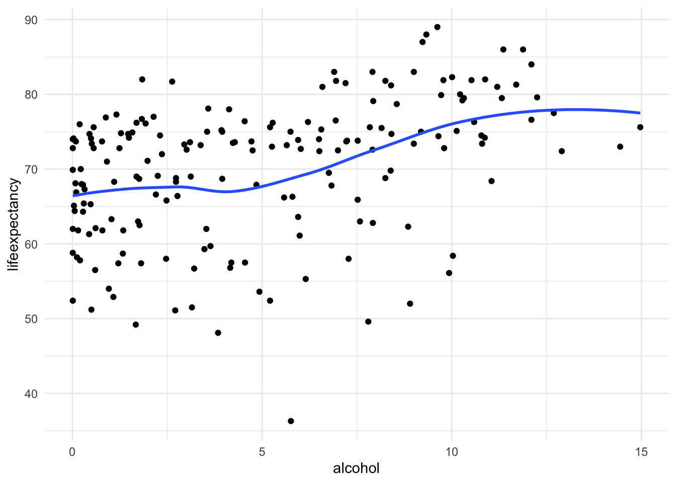
STEP 2: Generate log of variable
df_who <- df_who %>%
  mutate(log_alcohol = log(alcohol))
STEP 3: Check the skew and the new values
skewness(df_who$log_alcohol, na.rm = TRUE)[1] -1.648805As you can tell, logging the variable actually made skew worse. This is usually a good way of deciding if log is the right transformation. If your skew worsens/doesn’t get better, then either:
- You keep the variable as is but explain the decision not to skew.
- Create an alternate way of representing your variable, like turning it categorical.
Example 2: GDP
Let’s look at an example where we do want to move forward with the logged variable.
STEP 1: Check to see if your variable has heavy skew.
skewness(df_who$gdp, na.rm = TRUE)[1] 3.144006Here we see that gdp has a heavy skew. Income, wealth, and related measures are very often skewed. You can thank growing income inequality for that.
[Optional STEP]: Check the nature of relationship
ggplot(df_who, aes(x = gdp, y = lifeexpectancy)) +
  geom_point() +
  geom_smooth(method = "loess", se = FALSE) +
  theme_minimal()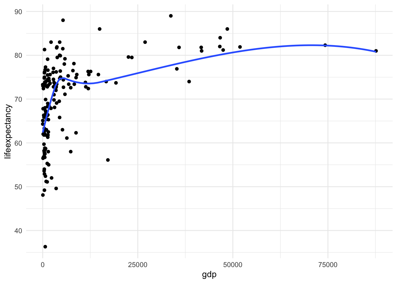
Here we also see the huge skew and resulting nonlinearity. The skew is the first thing we want to address.
STEP 2: Generate log of variable
df_who <- df_who %>%
  mutate(log_gdp = log(gdp))
STEP 3: Check the skew and the new values
skewness(df_who$log_gdp, na.rm = TRUE)[1] -0.3275022We fixed the skew! Let’s take a look at the new scatterplot too.
ggplot(df_who, aes(x = log_gdp, y = lifeexpectancy)) +
  geom_point() +
  geom_smooth(method = "loess", se = FALSE) +
  theme_minimal()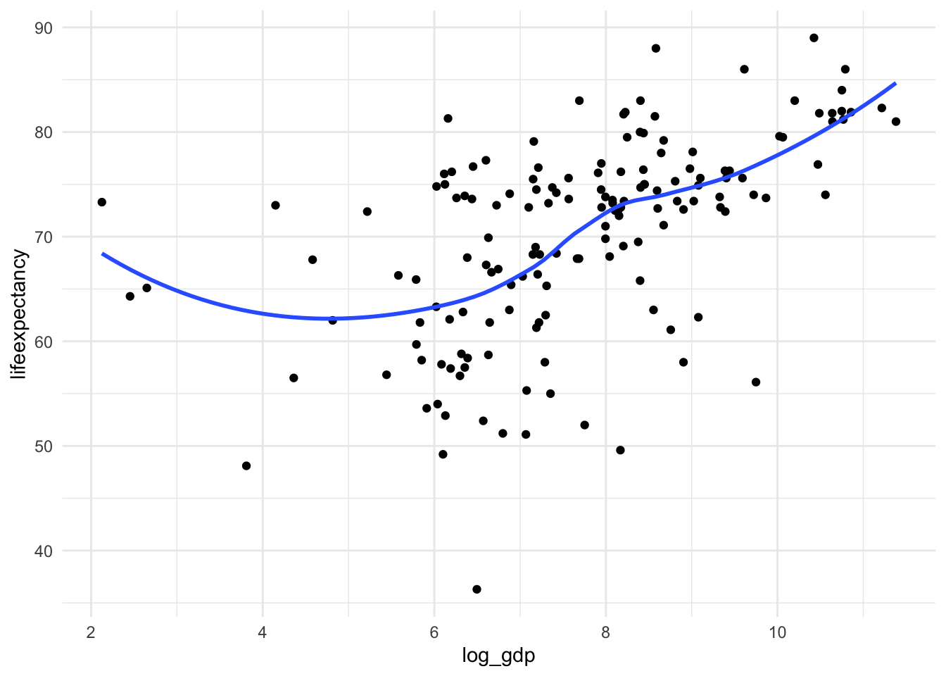
Not perfect, but much better!
Interpreting Logged Variables
When we log variables, we get some additional options for interpretation. Here’s a quick recap:
Log your independent variable (x): Divide the beta (aka coefficient) by 100 to interpret changes in X as “a 1% increase in X”
Log your dependent variable (y): Multiply the coefficient by 100 to interpret changes in Y as “a 1% change in Y”
Log both X and Y: You don’t need to do anything to the coefficient. Interpret changes as “a 1% increase in X is associated with a 1% change in Y”
Logged X Variables
STEP 1: Run the regression with the logged variable
fit3 <- lm(lifeexpectancy ~ log_gdp + total_hlth + alcohol +  schooling,
           data = df_who)
summary(fit3)
Call:
lm(formula = lifeexpectancy ~ log_gdp + total_hlth + alcohol +
    schooling, data = df_who)

Residuals:
     Min       1Q   Median       3Q      Max
-23.5795  -3.8292   0.4073   3.7422  14.4303

Coefficients:
            Estimate Std. Error t value Pr(>|t|)
(Intercept)  33.8591     2.4710  13.703  < 2e-16 ***
log_gdp       0.5546     0.3334   1.664  0.09830 .
total_hlth    0.3435     0.1924   1.785  0.07625 .
alcohol      -0.5042     0.1532  -3.290  0.00125 **
schooling     2.5889     0.2168  11.942  < 2e-16 ***
---
Signif. codes:  0 '***' 0.001 '**' 0.01 '*' 0.05 '.' 0.1 ' ' 1

Residual standard error: 5.593 on 150 degrees of freedom
  (28 observations deleted due to missingness)
Multiple R-squared:  0.6539,    Adjusted R-squared:  0.6447
F-statistic: 70.85 on 4 and 150 DF,  p-value: < 2.2e-16
STEP 2: Look up the names of your coefficients To refer to our coefficients we need to know the order they appear in our results. We can do this by calling the model results and the column “coefficients” in our results.
fit3$coefficients(Intercept) log_gdp total_hlth alcohol schooling
33.8590765 0.5546356 0.3434970 -0.5041866 2.5889180 STEP 3: Save your logged coefficient as an object.
Each coefficient can be referred to by it’s order in this list. So the
(Intercept) is 1, log_gdp is 2, total_hlth is 3, and so on.
We want to interpret log_gdp, which is the 2nd coefficient. You can call
up that coefficient by running:
fit3$coefficients[2] log_gdp
0.5546356 To do some basic math with this coefficient, let’s save it as a numeric object:
beta_logdp <- as.numeric(fit3$coefficients[2])STEP 4: Calculate the change in Y for a 1% change in X
In this case, because we’ve logged our independent variable, we want to
divide the coefficient by 100 to get the effect of a 1% change in gdp.
beta_logdp / 100[1] 0.005546356INTERPRETATION
A 1% change in gdp is associated with a 0.006 increase in life expectancy
OPTIONAL STEP: Go from 1% to 10% In this case, a 1% change in gdp isn’t associated with a super meaningful change in life expectancy. What does a 10% change in gdp look like? Let’s do some quick math.
What do we multiply 1 by to get to 10? Aka solve: 1 * x = 10 Answer - We multiply it by 10!
Dividing our coefficient by 100 is the same as multiplying by 1/100. We can multiply that by 10 to get to a 10% change.
1/100 * 10 = 1/10! So instead of dividing our coefficient by 100, we divide it by 10.
beta_logdp / 10[1] 0.05546356INTERPRETATION
A 10% change in gdp is associated with a 0.05 increase in life expectancy
Logged Outcome Variable
STEP 1: Generate the logged variable and run the regression
df_who <- df_who %>%
  mutate(log_lifeexpectancy = log(lifeexpectancy))

fit4 <- lm(log_lifeexpectancy ~ gdp + total_hlth + alcohol + schooling,
           data = df_who)
STEP 2: Save the coefficient as a numeric object
beta_gdp <- as.numeric(fit4$coefficients[2])STEP 3: Calculate the % change in Y
Multiply the coefficient of interest by 100 to change y to percentage.
beta_gdp * 100[1] 3.489947e-05INTERPRETATION
A 1 point increase GDP is associated with a .0003% increase in life expectancy.
Both Independent and Outcome Variables Logged
STEP 1: Run the regression
fit5 <- lm(log_lifeexpectancy ~ log_gdp + total_hlth + alcohol + schooling,
           data = df_who)
STEP 2: Interpret the results as percent changes
We don’t have to do any calculations when both the independent and dependent variables are logged. It just affects our interpretation.
summary(fit5)
Call:
lm(formula = log_lifeexpectancy ~ log_gdp + total_hlth + alcohol +
    schooling, data = df_who)

Residuals:
     Min       1Q   Median       3Q      Max
-0.49009 -0.05215  0.01120  0.05984  0.20048

Coefficients:
             Estimate Std. Error t value Pr(>|t|)
(Intercept)  3.701192   0.039863  92.847  < 2e-16 ***
log_gdp      0.007394   0.005379   1.375  0.17129
total_hlth   0.004567   0.003104   1.471  0.14335
alcohol     -0.008568   0.002472  -3.465  0.00069 ***
schooling    0.039697   0.003497  11.351  < 2e-16 ***
---
Signif. codes:  0 '***' 0.001 '**' 0.01 '*' 0.05 '.' 0.1 ' ' 1

Residual standard error: 0.09024 on 150 degrees of freedom
  (28 observations deleted due to missingness)
Multiple R-squared:  0.6169,    Adjusted R-squared:  0.6067
F-statistic:  60.4 on 4 and 150 DF,  p-value: < 2.2e-16
INTERPRETATION
A 1% percentage increase in gdp is associated with a 0.007 % percentage in life expectancy
Plotting Logged Variables with Margins
You can also use the ggpredict() function to display the results of your regression back in their original units.
Now for this to work, instead of creating a logged variable, we can just log our variable in the regression code.
fit6 <- lm(log(lifeexpectancy) ~ gdp + total_hlth + alcohol + schooling,
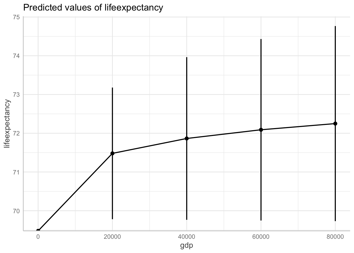
data = df_who)Show logged outcome in graph. Note we get the message about our logged variable. The command automatically backtransforms logged units into their original scale!
ggpredict(fit6, terms = "gdp[0:87700 by = 20000]") %>%
  plot(ci.style = "errorbar")
Model has log-transformed response. Back-transforming predictions to original response scale. Standard errors are still on the log-scale.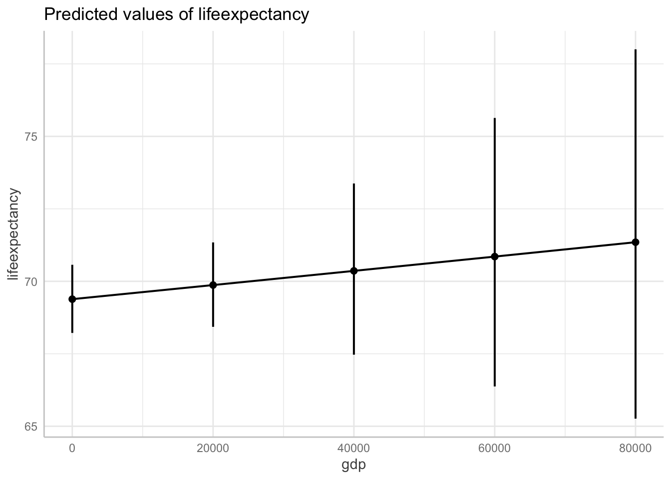
The same thing works for log-transformed covariates.
fit7 <- lm(lifeexpectancy ~ log(gdp) + total_hlth + alcohol + schooling,
           data = df_who)

ggpredict(fit7, terms = "gdp[0:87700 by = 20000]") %>%
  plot(ci.style = "errorbar")