14 Lab 7 (Stata)
14.1 Lab Goals & Instructions
Today we are using two datasets. We’ll load the dataset we need at different points in the lab.
Goals
- Use robust standard errors to address heteroskedasticity in your models
- Check the VIF for your model to detect multicollinearity
- Review interpretation of log transformed variables
Instructions
- Download the data and the script file from the lab files below.
- Run through the script file and reference the explanations on this page if you get stuck.
- No challenge activity!
Jump Links to Commands in this Lab:
14.2 Robust Standard Errors
We’re going to use two datasets in this lab. So let’s practice loading different datasets throughout our code. First, we’re going to load the UM DEI survey data:
use "data_raw/UM_DEIStudentSurvey.dta"Heteroskedasticity is a complicated word with a simple solution:
Robust Standard Errors!
Remember that heteroskedascity occurs when our constant variance is violated. Though it doesn’t bias our coefficients, it does affect our t-statistics and standard errors. That means something could appear significant when it is not.
To address this issue, we simply add ‘robust’ to the end of our regression. Compare these two equations, one with and one without standard errors.
STEP 1: Regression without robust standard errors
regress satisfaction climate_gen climate_dei instcom undergrad female i.race_5 Source | SS df MS Number of obs = 1,428
-------------+---------------------------------- F(9, 1418) = 126.80
Model | 681.762432 9 75.7513813 Prob > F = 0.0000
Residual | 847.152834 1,418 .597427951 R-squared = 0.4459
-------------+---------------------------------- Adj R-squared = 0.4424
Total | 1528.91527 1,427 1.07141925 Root MSE = .77293
-------------------------------------------------------------------------------
satisfaction | Coefficient Std. err. t P>|t| [95% conf. interval]
--------------+----------------------------------------------------------------
climate_gen | .5236206 .0377605 13.87 0.000 .4495482 .597693
climate_dei | .1331398 .0389881 3.41 0.001 .0566592 .2096204
instcom | .2901375 .0329719 8.80 0.000 .2254586 .3548165
undergrad | -.0150908 .0430709 -0.35 0.726 -.0995804 .0693987
female | -.0655309 .0426815 -1.54 0.125 -.1492566 .0181948
|
race_5 |
AAPI | -.0549904 .0572654 -0.96 0.337 -.1673244 .0573435
Black | -.4288251 .0681961 -6.29 0.000 -.5626011 -.2950491
Hispanic/L~o | -.1136751 .0592455 -1.92 0.055 -.2298933 .0025431
Other | -.118543 .0739411 -1.60 0.109 -.2635887 .0265027
|
_cons | .44564 .1332808 3.34 0.001 .1841914 .7070887
-------------------------------------------------------------------------------STEP 2: Check for heteroskedasticity You will need to predict your residuals, fitted values, and standardized residuals
    predict r1, residuals
    predict yhat
    predict rs, rstandard
    gen rs_sqrt = sqrt(rs)
And then look at the Residuals vs Fitted Values Plot:
scatter r1 yhat, yline(0) 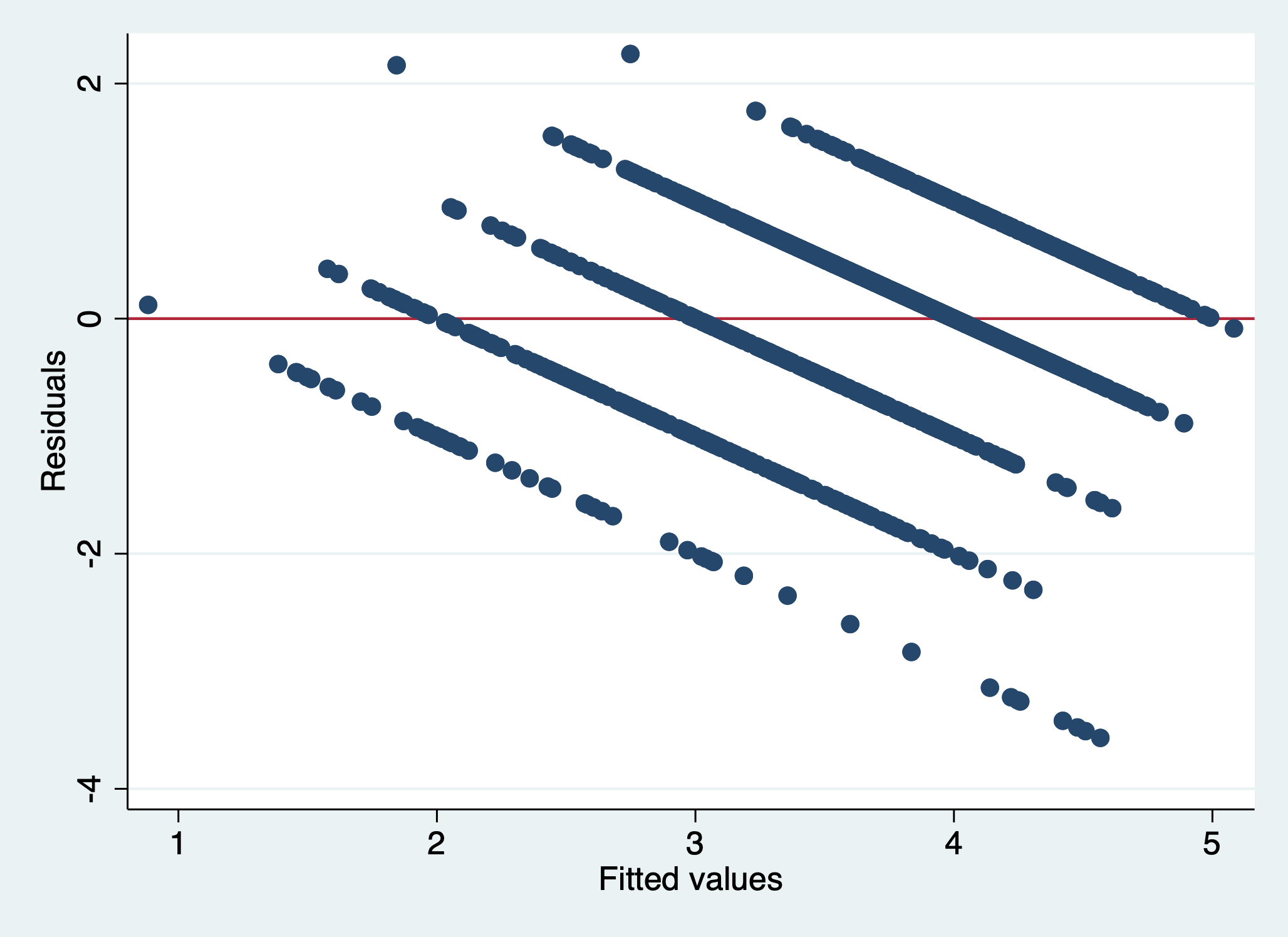
And the Standardized Residuals vs Predicted (Fitted) Values Plot
scatter rs_sqrt yhat || lowess rs_sqrt yhat 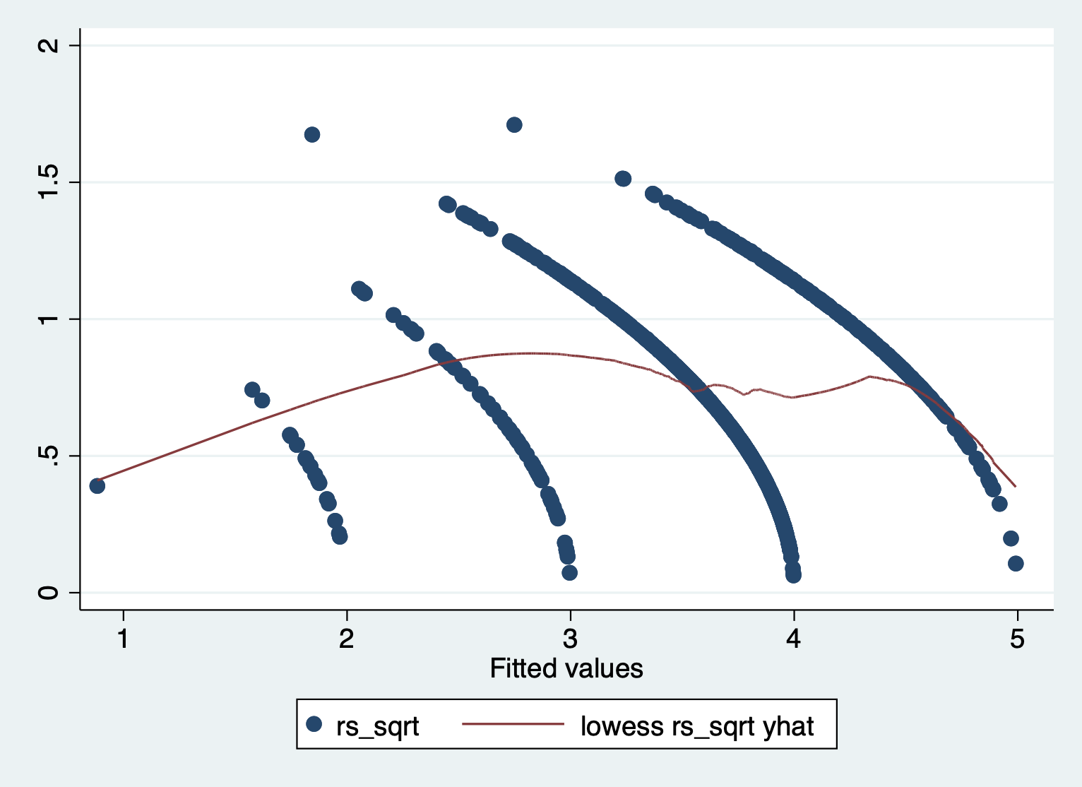
We can see that there is a pattern to the residuals and the standardized residuals plot does not have a flat horizontal line. Note: The residuals appear in lines because our outcome is technically categorical and we are treating it as if it were continuous.
STEP 3: Regression with robust standard errors
regress satisfaction climate_gen climate_dei instcom undergrad female i.race_5, robust> , robust
Linear regression Number of obs = 1,428
F(9, 1418) = 142.30
Prob > F = 0.0000
R-squared = 0.4459
Root MSE = .77293
-------------------------------------------------------------------------------
| Robust
satisfaction | Coefficient std. err. t P>|t| [95% conf. interval]
--------------+----------------------------------------------------------------
climate_gen | .5236206 .0436841 11.99 0.000 .4379282 .609313
climate_dei | .1331398 .0437796 3.04 0.002 .04726 .2190195
instcom | .2901375 .0357382 8.12 0.000 .220032 .360243
undergrad | -.0150908 .042187 -0.36 0.721 -.0978465 .0676648
female | -.0655309 .0417799 -1.57 0.117 -.1474879 .0164261
|
race_5 |
AAPI | -.0549904 .0542679 -1.01 0.311 -.1614444 .0514635
Black | -.4288251 .0677889 -6.33 0.000 -.5618024 -.2958478
Hispanic/L~o | -.1136751 .0584993 -1.94 0.052 -.2284295 .0010793
Other | -.118543 .0818023 -1.45 0.148 -.2790095 .0419235
|
_cons | .44564 .1263582 3.53 0.000 .1977709 .6935092
-------------------------------------------------------------------------------QUESTION: What changes? Based on these changes, how serious was heteroskedascity in this model?
Adding the robust standard errors doesn’t change that much in the model. You will see that the coefficients do not change, but the standard errors do. The changed standard errors then affect the t scores and p-values.
How bad does heteroskedasticity need to be to use robust standard errors?
The rule of thumb is that robust standard errors are the best almost all the time. Unless you see near perfect variance around 0 when you plot your residuals, it is always best to use robust standard errors.
!! Better safe than sorry!!
14.3 Detecting Multicollinearity
Multicollinearity occurs when some of your independent variables are too closely correlated with one another. When this happens, the model can’t separate the effects of each variable because they always vary together.
Checking for multicollinearity is a fairly straightforward process. What we do is check the VIF of our model after we run a regression. When a VIF is greater than 10, that is an indication that there is multicollinearity.
Example 1
First, run the regression. I’m not going to show the results here because I want you to focus on the results of the VIF.
regress satisfaction climate_gen climate_dei instcom undergrad female i.race_5After you run the regression, execute this simple two word command:
estat vif Variable | VIF 1/VIF
-------------+----------------------
climate_gen | 1.82 0.549942
climate_dei | 2.41 0.415174
instcom | 1.88 0.531935
undergrad | 1.09 0.921261
female | 1.08 0.922795
race_5 |
2 | 1.21 0.829711
3 | 1.26 0.794073
4 | 1.18 0.846844
5 | 1.13 0.882257
-------------+----------------------
Mean VIF | 1.45What we find here is that our model has very little multicollinearity because everything in our model has a vif (variance inflation factor) that is below 10.
Example 2
Let’s take a look at one example where you might see higher vif.
regress satisfaction climate_gen climate_dei instcom c.instcom#c.instcom undergrad female i.race_5estat vif Variable | VIF 1/VIF
-------------+----------------------
climate_gen | 1.90 0.527393
climate_dei | 2.41 0.414748
instcom | 37.22 0.026869
c.instcom#|
c.instcom | 35.19 0.028418
undergrad | 1.09 0.920450
female | 1.09 0.919378
race_5 |
2 | 1.21 0.827686
3 | 1.26 0.792306
4 | 1.18 0.846778
5 | 1.14 0.880746
-------------+----------------------
Mean VIF | 8.37As you can see, adding a polynomial can increase your vif (above 10 and close to 30). We generally recognize a polynomial will have a high vif, so we can pay attention to the other variables to determine multicollinearity.
When you find yourself in this scenario, I suggest two approaches:
Double check the final vif average for the model. If its still under 10, then you definitely safe to keep the polynomial in the model.
If it sends the ‘mean vif’ over 10, one thing to do is to take the polynomial out temporarily. Check the vif of that model to evaluate multicollinearity, and then make your decision before you add the polynomial.
14.4 Interpreting Logged Variables (Review)
Now we need to switch datasets. To do this we have to first clear our environment of the existing dataset, and then we can load the WHO life expectancy data.
clear all
use "data_raw/who_life_expectancy_2010.dta"
Logging Variables
First, we are reviewing how to log variables. The steps of logging a variable is pretty simple. We’re going to run through two examples.
Example 1: Alcohol Consumption
STEP 1: Check to see if your variable has heavy skew.
sum alcohol, d Alcohol consumption per capita (litres)
-------------------------------------------------------------
Percentiles Smallest
1% .01 .01
5% .08 .01
10% .28 .01 Obs 182
25% 1.34 .01 Sum of wgt. 182
50% 4.21 Mean 4.943626
Largest Std. dev. 3.889271
75% 7.93 12.69
90% 10.52 12.9 Variance 15.12643
95% 11.36 14.44 Skewness .4261967
99% 14.44 14.97 Kurtosis 2.036435General Rule: if skew is greater than 1 or less than -1, consider logging. Though this doesn’t meet that extreme skew, we will still carry forward with the possibility of logging the variable.
[Optional STEP]: Check the nature of relationship
If you aren’t sure what type of relationship this is already, you might
consider checking a scatter to make sure this a different nonlinearity
i.e. cubic polynomial.
scatter lifeexpectancy alcohol || lowess lifeexpectancy alcohol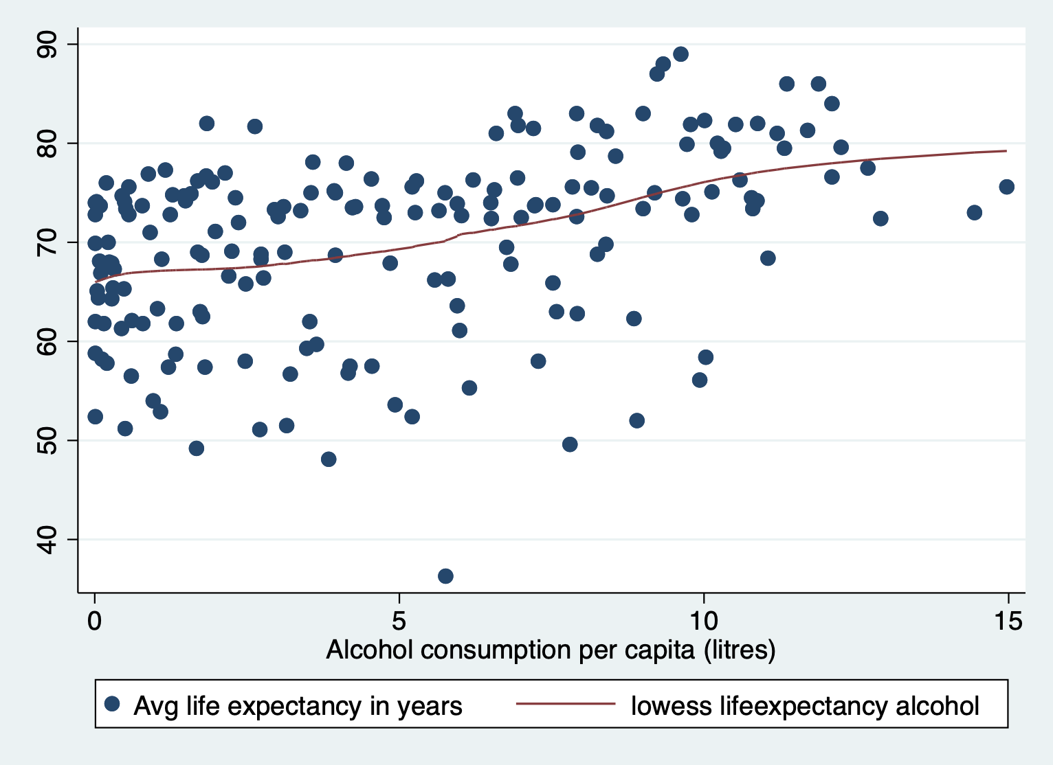
STEP 2: Generate log of variable
gen log_alcohol = log(alcohol)STEP 3: Check the skew and the new values
sum log_alcohol, d log_alcohol
-------------------------------------------------------------
Percentiles Smallest
1% -4.60517 -4.60517
5% -2.525729 -4.60517
10% -1.272966 -4.60517 Obs 182
25% .2926696 -4.60517 Sum of wgt. 182
50% 1.437451 Mean .9107274
Largest Std. dev. 1.656438
75% 2.070653 2.540814
90% 2.353278 2.557227 Variance 2.743785
95% 2.430098 2.670002 Skewness -1.648805
99% 2.670002 2.706048 Kurtosis 5.510823As you can tell, logging the variable actually made skew worse. This is usually a good way of deciding if log is the right transformation. If your skew worsens/doesn’t get better, then either:
- You keep the variable as is but explain the decision not to skew.
- Create an alternate way of representing your variable, like turning it categorical.
Example 2: GDP
Let’s look at an example where we do want to move forward with the logged variable.
STEP 1: Check to see if your variable has heavy skew.
sum gdp, d Gross Domestic Product (GDP) per capita in USD
-------------------------------------------------------------
Percentiles Smallest
1% 11.63138 8.376432
5% 123.3837 11.63138
10% 369.2393 14.14227 Obs 156
25% 687.9576 45.12842 Sum of wgt. 156
50% 2183.358 Mean 7464.488
Largest Std. dev. 13959.52
75% 5842.135 48538.59
90% 22538.65 51874.85 Variance 1.95e+08
95% 41785.56 74276.72 Skewness 3.144006
99% 74276.72 87646.75 Kurtosis 13.87194Here we see that gdp has a heavy skew. Income, wealth, and related measures are very often skewed. You can thank growing income inequality for that.
[Optional STEP]: Check the nature of relationship
scatter lifeexpectancy gdp || lowess lifeexpectancy gdp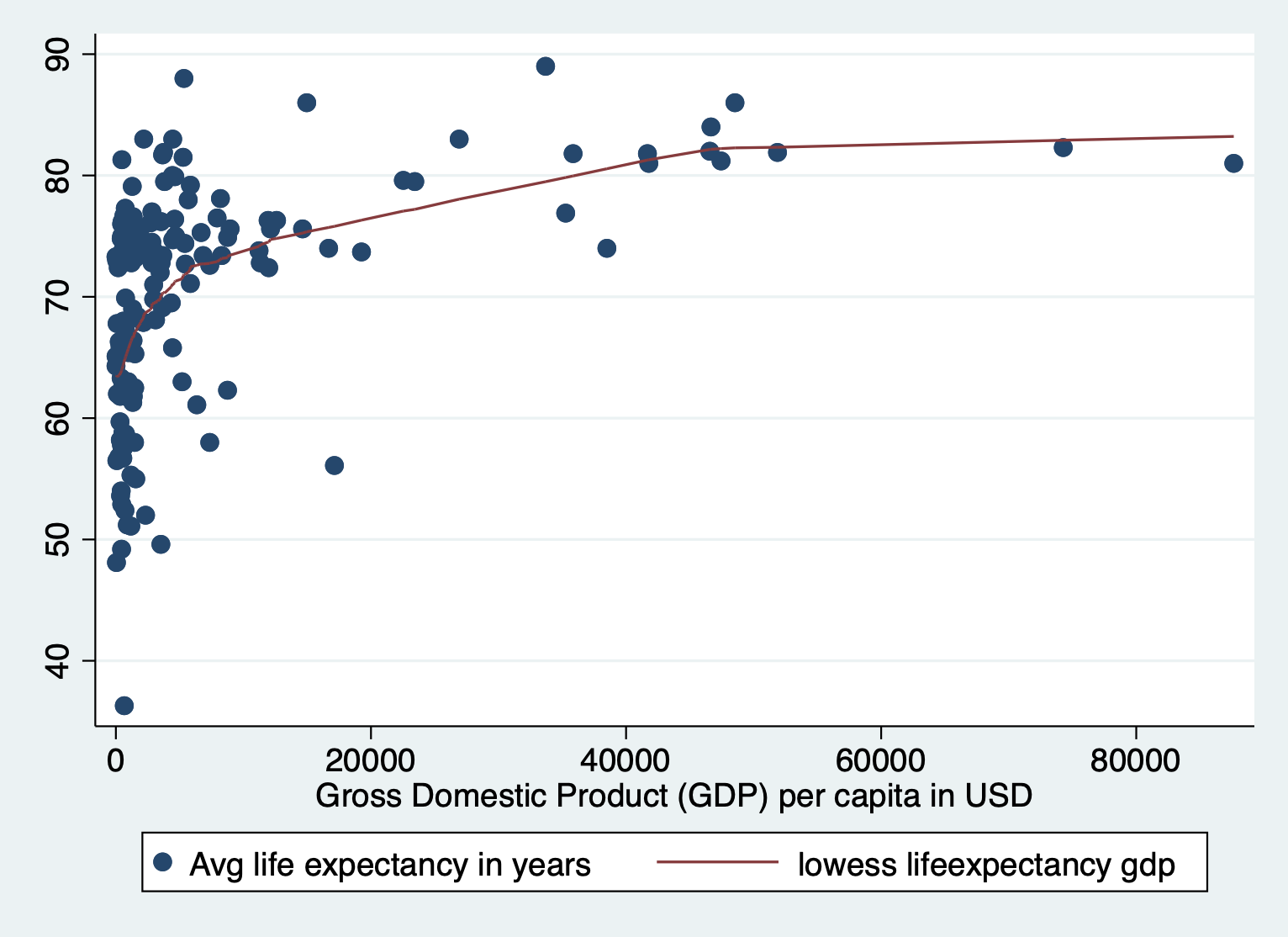
Here we also see the huge skew and resulting nonlinearity. The skew is the first thing we want to address.
STEP 2: Generate log of variable
gen log_gdp = log(gdp)STEP 3: Check the skew and the new values
sum log_gdp, d log_gdp
-------------------------------------------------------------
Percentiles Smallest
1% 2.453706 2.125422
5% 4.815299 2.453706
10% 5.911445 2.649168 Obs 156
25% 6.53303 3.809512 Sum of wgt. 156
50% 7.688617 Mean 7.678683
Largest Std. dev. 1.70432
75% 8.672852 10.79011
90% 10.02299 10.85659 Variance 2.904708
95% 10.64031 11.21555 Skewness -.3275022
99% 11.21555 11.38107 Kurtosis 3.651007We fixed the skew! Let’s take a look at the new scatterplot too.
scatter lifeexpectancy log_gdp || lowess lifeexpectancy log_gdp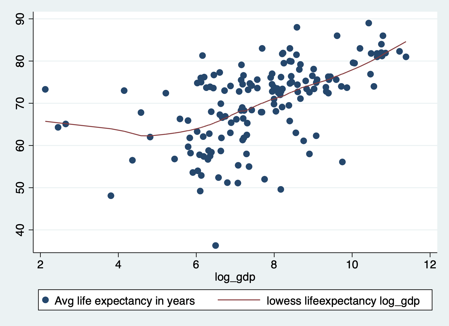
Not perfect, but much better!
Interpreting Logged Variables
When we log variables, we get some additional options for interpretation. Here’s a quick recap:
Log your independent variable (x): Divide the beta (aka coefficient) by 100 to interpret changes in X as “a 1% increase in X”
Log your dependent variable (y): Multiply the coefficient by 100 to interpret changes in Y as “a 1% change in Y”
Log both X and Y: You don’t need to do anything to the coefficient. Interpret changes as “a 1% increase in X is associated with a 1% change in Y”
Logged X Variables
STEP 1: Run the regression with the logged variable
regress lifeexpectancy log_gdp total_hlth alcohol schooling Source | SS df MS Number of obs = 155
-------------+---------------------------------- F(4, 150) = 70.85
Model | 8865.92867 4 2216.48217 Prob > F = 0.0000
Residual | 4692.93818 150 31.2862546 R-squared = 0.6539
-------------+---------------------------------- Adj R-squared = 0.6447
Total | 13558.8669 154 88.04459 Root MSE = 5.5934
------------------------------------------------------------------------------
lifeexpect~y | Coefficient Std. err. t P>|t| [95% conf. interval]
-------------+----------------------------------------------------------------
log_gdp | .5546356 .333414 1.66 0.098 -.1041588 1.21343
total_hlth | .343497 .1924155 1.79 0.076 -.0366977 .7236917
alcohol | -.5041866 .1532459 -3.29 0.001 -.8069861 -.2013872
schooling | 2.588918 .216783 11.94 0.000 2.160575 3.017261
_cons | 33.85908 2.47096 13.70 0.000 28.97669 38.74146
------------------------------------------------------------------------------STEP 2: Look up the names of your coefficients
coeflegend is a command that allows you to see the label for your beta coefficient. This is useful if you need to do calculations with it later. You can just put put the model command you just ran, then put coeflegend to display the beta names.
regress, coeflegend Source | SS df MS Number of obs = 155
-------------+---------------------------------- F(4, 150) = 70.85
Model | 8865.92867 4 2216.48217 Prob > F = 0.0000
Residual | 4692.93818 150 31.2862546 R-squared = 0.6539
-------------+---------------------------------- Adj R-squared = 0.6447
Total | 13558.8669 154 88.04459 Root MSE = 5.5934
------------------------------------------------------------------------------
lifeexpect~y | Coefficient Legend
-------------+----------------------------------------------------------------
log_gdp | .5546356 _b[log_gdp]
total_hlth | .343497 _b[total_hlth]
alcohol | -.5041866 _b[alcohol]
schooling | 2.588918 _b[schooling]
_cons | 33.85908 _b[_cons]
------------------------------------------------------------------------------STEP 3: Calculate the change in Y for a 1% change in X
In this case, because we’ve logged our independent variable, we want to
divide the coefficient by 100 to get the effect of a 1% change in gdp.
display _b[log_gdp] / 100 .00554636INTERPRETATION
A 1% change in gdp is associated with a 0.006 increase in life expectancy
OPTIONAL STEP: Go from 1% to 10% In this case, a 1% change in gdp isn’t associated with a super meaningful change in life expectancy. What does a 10% change in gdp look like? Let’s do some quick math.
What do we multiply 1 by to get to 10? Aka solve: 1 * x = 10 Answer - We multiply it by 10!
Dividing our coefficient by 100 is the same as multiplying by 1/100. We can multiply that by 10 to get to a 10% change.
1/100 * 10 = 1/10! So instead of dividing our coefficient by 100, we divide it by 10.
display _b[log_gdp] / 10 .05546356INTERPRETATION
A 10% change in gdp is associated with a 0.05 increase in life expectancy
Logged Outcome Variable
STEP 1: Generate the logged variable and run the regression
gen log_lifeexpectancy = log(lifeexpectancy)
regress log_lifeexpectancy gdp total_hlth alcohol schooling
Source | SS df MS Number of obs = 155
-------------+---------------------------------- F(4, 150) = 59.38
Model | 1.95435382 4 .488588455 Prob > F = 0.0000
Residual | 1.23418684 150 .008227912 R-squared = 0.6129
-------------+---------------------------------- Adj R-squared = 0.6026
Total | 3.18854066 154 .020704809 Root MSE = .09071
------------------------------------------------------------------------------
log_lifeex~y | Coefficient Std. err. t P>|t| [95% conf. interval]
-------------+----------------------------------------------------------------
gdp | 3.49e-07 6.19e-07 0.56 0.574 -8.75e-07 1.57e-06
total_hlth | .004638 .0031813 1.46 0.147 -.0016479 .0109239
alcohol | -.0084138 .002484 -3.39 0.001 -.013322 -.0035057
schooling | .0412849 .0033431 12.35 0.000 .0346792 .0478906
_cons | 3.734208 .039293 95.03 0.000 3.656568 3.811847
------------------------------------------------------------------------------STEP 2: Calculate the % change in Y
Multiply the coefficient of interest by 100 to change y to percentage.
display _b[gdp]3.490e-07INTERPRETATION
A 1 point increase GDP is associated with a .0003% increase in life expectancy.
Both Independent and Outcome Variables Logged
STEP 1: Run the regression
regress log_lifeexpectancy log_gdp total_hlth alcohol schooling Source | SS df MS Number of obs = 155
-------------+---------------------------------- F(4, 150) = 60.40
Model | 1.96712861 4 .491782153 Prob > F = 0.0000
Residual | 1.22141204 150 .008142747 R-squared = 0.6169
-------------+---------------------------------- Adj R-squared = 0.6067
Total | 3.18854066 154 .020704809 Root MSE = .09024
------------------------------------------------------------------------------
log_lifeex~y | Coefficient Std. err. t P>|t| [95% conf. interval]
-------------+----------------------------------------------------------------
log_gdp | .0073941 .0053789 1.37 0.171 -.0032341 .0180223
total_hlth | .0045667 .0031042 1.47 0.143 -.0015669 .0107003
alcohol | -.0085676 .0024723 -3.47 0.001 -.0134526 -.0036826
schooling | .0396967 .0034973 11.35 0.000 .0327863 .046607
_cons | 3.701192 .0398634 92.85 0.000 3.622426 3.779959
------------------------------------------------------------------------------STEP 2: Interpret the results as percent changes
We don’t have to do any calculations when both the independent and dependent variables are logged. It just affects our interpretation.
INTERPRETATION
A 1% percentage increase in gdp is associated with a 0.007 % percentage in life expectancy
Plotting Logged Variables with Margins
You can also use margins to exponentiate from logged to unlogged units (your original y units) using margins. The way to do that is…
First, run the regression. I’m not going to display the results of the regression so you focus on the margins plots.
regress log_lifeexpectancy gdp total_hlth alcohol schoolingHere’s what the margins plot looks like when we keep the outcome variable in logged units. I’m running the margins quietly because I just want to look at the plot.
quietly margins, at(gdp =(0(20000)87700))
marginsplot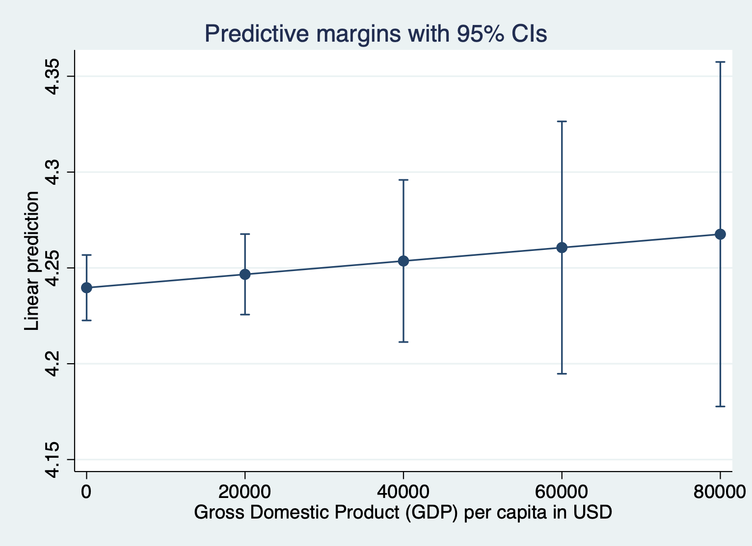
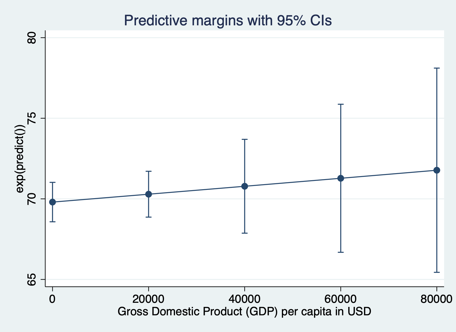
Here’s what it looks like to show the unlogged units for the outcome. We have to include expression(exp(predict())) after the comma. Everything else about the command is the same.
quietly margins, expression(exp(predict())) at(gdp =(0(20000)87700))
marginsplot