11 Lab 5 (R)
11.1 Lab Goals & Instructions
Today we are back to using the billionaires dataset.
Research Question: What characteristics are associated with wealth among billionaires?
Goals
- Produce journal-ready tables in Stata (or at least close to journal-ready)
Instructions
- Download the data and the script file from the lab files below.
- Run through the script file and reference the explanations on this page if you get stuck.
- Work on the challenge activity if you have time.
Libraries
# Load libraries
library(tidyverse)

# The three libraries we'll be using in this lab
# You should also install the package "flextable"
library(gtsummary)
library(stargazer)
library(huxtable)
# install.packages("flextable")
Jump Links to Commands in this Lab:
11.2 Saving Models
In Stata we have to download a new package to save the results from our regressions. In R, we save results as objects in the environment pretty regularly. To make building tables easy, make sure you save your results as objects.
m1 <- lm(wealthworthinbillions ~ female + age, data = mydata)
summary(m1)
Call:
lm(formula = wealthworthinbillions ~ female + age, data = mydata)

Residuals:
   Min     1Q Median     3Q    Max
-3.764 -2.217 -1.507 -0.091 72.480

Coefficients:
            Estimate Std. Error t value Pr(>|t|)
(Intercept) 1.461568   0.557531   2.622  0.00881 **
female      0.430905   0.389897   1.105  0.26920
age         0.035492   0.008692   4.083  4.6e-05 ***
---
Signif. codes:  0 '***' 0.001 '**' 0.01 '*' 0.05 '.' 0.1 ' ' 1

Residual standard error: 5.388 on 2226 degrees of freedom
  (385 observations deleted due to missingness)
Multiple R-squared:  0.007916,  Adjusted R-squared:  0.007025
F-statistic: 8.881 on 2 and 2226 DF,  p-value: 0.000144
11.3 Building Tables
In this section, we will focus on three packages you can use to build and export tables: stargazer, gtsummary, and huxtable. We’ll cover their basics, as well as changes you can make to the visual of the table.
Here are some more resources for each:
- stargazer: https://www.jakeruss.com/cheatsheets/stargazer/
- gtsummary: https://www.danieldsjoberg.com/gtsummary/
- huxtable: https://ramorel.github.io/posts/reg-tables-huxtable/
11.3.1 Tables with stargazer
Stargazer is a relatively straightforward package that can build nice tables. It’s pros are its simplicity and ability to be used in R markdown. It’s cons are that it’s hard to export in word format and not quite as flexible as our final option. This is the package I see recommended most for building regression tables.
Regression tables with stargazer
To build a regression table in this package, we use the function stargazer() and putting your saved model results into the function.
You will also need to specify a type in the command, either “text” or “html.”
Text will allow you to see the output in a regular script file. Html will
show up better in an Rmarkdown file.
Let’s start by producing a simple table from the model we already saved in text format:
stargazer(m1, type = "text")
===============================================
                        Dependent variable:
                    ---------------------------
                       wealthworthinbillions
-----------------------------------------------
female                         0.431
                              (0.390)

age                          0.035***
                              (0.009)

Constant                     1.462***
                              (0.558)

-----------------------------------------------
Observations                   2,229
R2                             0.008
Adjusted R2                    0.007
Residual Std. Error      5.388 (df = 2226)
F Statistic           8.881*** (df = 2; 2226)
===============================================
Note:               *p<0.1; **p<0.05; ***p<0.01
Text format isn’t the best option for inserting a table into word, but if you wanted to
save it as a text file, you specify the file to create with the out = "filepath" option.
stargazer(m1, type = "text", out = "figs_output/example.txt")Now let’s try an html version. The output we see in our code is just html code. To look at it we need to save it to an html file. Here is our simple table in html format and how it will look when you open the file:
stargazer(m1, type = "html", out = "figs_output/example.htm")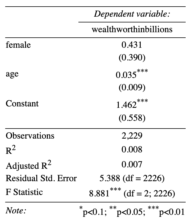
If you want to insert this table into a word document you can take a screenshot and save the table as an image. For this reason, stargazer is not my favorite package
Descriptive statistic tables with stargazer
Stargazer can also create descriptive statistic tables with the same stargazer() function. Instead of listing the model results in the function, you put in the name of your dataframe with the variables you want to appear in the table.
For some reason, this command only works if you explicitly save your dataframe as a dataframe.
mydata <- as.data.frame(mydata) %>%
  mutate(wealthtype2 = factor(wealthtype2,
                              labels = c("Executive",
                                         "Founder (non-finance)",
                                         "Inherited",
                                         "Privatized",
                                         "Self-made (finance)")))
Here’s a basic descriptive statistics table in text format:
stargazer(mydata, type = "text")
==========================================================================================================================
Statistic               N           Mean                St. Dev.         Min   Pctl(25)    Pctl(75)            Max
--------------------------------------------------------------------------------------------------------------------------
rank                  2,614        599.673               467.886          1      215          988             1,565
year                  2,614       2,008.412               7.484         1,996   2,001        2,014            2,014
companyfounded        2,614       1,924.712              243.777          0     1,936        1,985            2,012
demographicsage       2,614        53.341                25.333          -42      47          70                98
locationgdp           2,614 1,769,103,031,873.000 3,547,082,560,202.000   0       0     725,000,000,000 10,600,000,000,000
wealthworthinbillions 2,614         3.532                 5.089         1.000   1.400        3.500            76.000
wealthhowinherited2   2,614         4.386                 1.194           1       4            5                6
wealthhowcategory2    2,613         4.662                 1.651         1.000   3.000        6.000            9.000
wealthhowindustry2    2,613         8.715                 4.637         1.000   4.000       13.000            19.000
locationregion2       2,614         4.236                 1.720           1       3            6                8
locationcountrycode2  2,614        45.674                24.173           1       23          71                74
locationcitizenship2  2,614        46.764                23.861           1       23          71                73
demographicsgender2   2,580         1.905                 0.298         1.000   2.000        2.000            3.000
companysector2        2,591        271.851               143.659        1.000  132.000      402.000          520.000
companyrelationship2  2,568        45.266                18.268         1.000   32.000      66.000            74.000
age                   2,229        62.576                13.135         12.000  53.000      72.000            98.000
female                2,577         0.097                 0.296         0.000   0.000        0.000            1.000
--------------------------------------------------------------------------------------------------------------------------
You can also select specific variables using the tidyverse pipe (%>% select()) and which specific statistics should display. Here are the statistics options you have available:
n: Number of observationsmean: Meansd: Standard devaitionmin: Minimum valuemax: Maximum valuemedian: Medianp25: 25th percentile valuep75: 75th percentile value
These are all options in the command itself that you can set to TRUE or FALSE.
stargazer(
  mydata %>% select(wealthworthinbillions, wealthtype2, female, age),
  summary.stat = c("n", "mean", "sd", "min", "max"),
  type = "text"
)
=========================================================
Statistic               N    Mean  St. Dev.  Min    Max
---------------------------------------------------------
wealthworthinbillions 2,614 3.532   5.089   1.000  76.000
female                2,577 0.097   0.296   0.000  1.000
age                   2,229 62.576  13.135  12.000 98.000
---------------------------------------------------------
Variations on your stargazer tables
You can also add numerous options to your stargazer command to improve the look of the overall table. Some of the ones you’ll use most often are:
title: Add a table titlecovariate.labels: Add a label to the variables in your table instead of its name in your dataframe.dept.var.labels: Label the dependent variable in your modelcolumn.labels: When you have multiple models in your regression table, label each model (aka column).digits: Round to a certain number of decimals.
Here’s an example of a descriptive table with some specifications:
stargazer(
  mydata %>% select(wealthworthinbillions, wealthtype2, female, age),
  summary.stat = c("n", "mean", "sd", "min", "max"),
  type = "text",
  digits = 2, # round to 2 decimal points
  title = "Table 1. Descriptive Statistics", # add a title
  covariate.labels = c("Wealth (in billions)", "Wealth Type", "Female", "Age" )
)
Table 1. Descriptive Statistics
=====================================================
Statistic              N   Mean  St. Dev.  Min   Max
-----------------------------------------------------
Wealth (in billions) 2,614 3.53    5.09   1.00  76.00
Wealth Type          2,577 0.10    0.30   0.00  1.00
Female               2,229 62.58  13.13   12.00 98.00
-----------------------------------------------------
Note this does not handle categorical variables well. It is treating wealth type as a numeric variable.
Regression tables with multiple models with stargazer
Most journal tables will include more than one model. Stargazer has this capability, as do all the options we are looking at in this lab.
First, let’s run and save a second regression:
m2 <- lm(wealthworthinbillions ~ female + age + wealthtype2, data = mydata)Here’s the basic table with two models:
stargazer(m1, m2, type = "text")
================================================================================
                                               Dependent variable:
                                 -----------------------------------------------
                                              wealthworthinbillions
                                           (1)                     (2)
--------------------------------------------------------------------------------
female                                    0.431                   0.228
                                         (0.390)                 (0.414)

age                                     0.035***                0.039***
                                         (0.009)                 (0.009)

wealthtype2Founder (non-finance)                                1.294***
                                                                 (0.467)

wealthtype2Inherited                                            1.236***
                                                                 (0.466)

wealthtype2Privatized                                           1.447***
                                                                 (0.555)

wealthtype2Self-made (finance)                                    0.413
                                                                 (0.487)

Constant                                1.462***                  0.275
                                         (0.558)                 (0.696)

--------------------------------------------------------------------------------
Observations                              2,229                   2,227
R2                                        0.008                   0.015
Adjusted R2                               0.007                   0.012
Residual Std. Error                 5.388 (df = 2226)       5.377 (df = 2220)
F Statistic                      8.881*** (df = 2; 2226) 5.583*** (df = 6; 2220)
================================================================================
Note:                                                *p<0.1; **p<0.05; ***p<0.01
And here’s the two model table with specifications:
stargazer(m1, m2,
          type = "text",
          digits = 2,
          dep.var.labels = c("Wealth (in billions)"), # Label dep variable
          # Covariate labels
          covariate.labels = c("Female", "Age", "Wealth Type: Founder",
                               "Wealth Type: Inherited",
                               "Wealth Type: Privatized",
                               "Wealth Type: Self-made (finance)"),
          # Name the models
          column.labels = c("Model 1", "Model 2")
          )
==============================================================================
                                              Dependent variable:
                                 ---------------------------------------------
                                             Wealth (in billions)
                                        Model 1                Model 2
                                          (1)                    (2)
------------------------------------------------------------------------------
Female                                    0.43                   0.23
                                         (0.39)                 (0.41)

Age                                     0.04***                0.04***
                                         (0.01)                 (0.01)

Wealth Type: Founder                                           1.29***
                                                                (0.47)

Wealth Type: Inherited                                         1.24***
                                                                (0.47)

Wealth Type: Privatized                                        1.45***
                                                                (0.55)

Wealth Type: Self-made (finance)                                 0.41
                                                                (0.49)

Constant                                1.46***                  0.28
                                         (0.56)                 (0.70)

------------------------------------------------------------------------------
Observations                             2,229                  2,227
R2                                        0.01                   0.01
Adjusted R2                               0.01                   0.01
Residual Std. Error                 5.39 (df = 2226)       5.38 (df = 2220)
F Statistic                      8.88*** (df = 2; 2226) 5.58*** (df = 6; 2220)
==============================================================================
Note:                                              *p<0.1; **p<0.05; ***p<0.01
11.3.2 Tables with gtsummary
gtsummary is another relatively straightforward table building package.
It has the advantage of showing a nice html output It is also a great option for building summary statistics tables because it handles categorical variables much better. Cons are the options are much more complicated and split between in function options and
piped options and it can’t be exported directly to word.
Regression tables with gtsummary
The basic command we’ll be using from this package for regression tables is tbl_regression() and the saved model results.
tbl_regression(m2)| Characteristic | Beta | 95% CI1 | p-value |
|---|---|---|---|
| female | 0.23 | -0.58, 1.0 | 0.6 |
| age | 0.04 | 0.02, 0.06 | <0.001 |
| wealthtype2 | |||
| Executive | — | — | |
| Founder (non-finance) | 1.3 | 0.38, 2.2 | 0.006 |
| Inherited | 1.2 | 0.32, 2.2 | 0.008 |
| Privatized | 1.4 | 0.36, 2.5 | 0.009 |
| Self-made (finance) | 0.41 | -0.54, 1.4 | 0.4 |
|
1
CI = Confidence Interval
|
|||
Here is how you add labels to the covariates:
tbl_regression(m2,
               # Add variable labels
               label = c(female ~ "Female",
                         age ~ "Age",
                         wealthtype2 ~ "Wealth Type")
)| Characteristic | Beta | 95% CI1 | p-value |
|---|---|---|---|
| Female | 0.23 | -0.58, 1.0 | 0.6 |
| Age | 0.04 | 0.02, 0.06 | <0.001 |
| Wealth Type | |||
| Executive | — | — | |
| Founder (non-finance) | 1.3 | 0.38, 2.2 | 0.006 |
| Inherited | 1.2 | 0.32, 2.2 | 0.008 |
| Privatized | 1.4 | 0.36, 2.5 | 0.009 |
| Self-made (finance) | 0.41 | -0.54, 1.4 | 0.4 |
|
1
CI = Confidence Interval
|
|||
Regression tables with multiple models with gtsummary
To put two models together with this package, you have to save the separate tables as objects and then combine them with the tbl_merge() function.
So here we save the two models:
tbl1 <- tbl_regression(m1,
                       # Add variable labels
                       label = c(female ~ "Female",
                                 age ~ "Age"))
tbl2 <- tbl_regression(m2,
               # Add variable labels
               label = c(female ~ "Female",
                         age ~ "Age",
                         wealthtype2 ~ "Wealth Type"))
And here we put them together:
tbl_merge(
  list(tbl1, tbl2),
  tab_spanner = c("**Model 1**", "**Model 2**")
)| Characteristic | Model 1 | Model 2 | ||||
|---|---|---|---|---|---|---|
| Beta | 95% CI1 | p-value | Beta | 95% CI1 | p-value | |
| Female | 0.43 | -0.33, 1.2 | 0.3 | 0.23 | -0.58, 1.0 | 0.6 |
| Age | 0.04 | 0.02, 0.05 | <0.001 | 0.04 | 0.02, 0.06 | <0.001 |
| Wealth Type | ||||||
| Executive | — | — | ||||
| Founder (non-finance) | 1.3 | 0.38, 2.2 | 0.006 | |||
| Inherited | 1.2 | 0.32, 2.2 | 0.008 | |||
| Privatized | 1.4 | 0.36, 2.5 | 0.009 | |||
| Self-made (finance) | 0.41 | -0.54, 1.4 | 0.4 | |||
|
1
CI = Confidence Interval
|
||||||
Descriptive statistics tables with gtsummary
To create descriptive statistics tables with this package, we use the function tbl_summary and list the dataframe with the variables we want to summarize.
Here is a simple summary table, with selected variables from our data frame:
tbl_summary(
  mydata %>% select(wealthworthinbillions, female, age, wealthtype2)
)| Characteristic | N = 2,6141 |
|---|---|
| wealthworthinbillions | 2.0 (1.4, 3.5) |
| female | 249 (9.7%) |
| Unknown | 37 |
| age | 62 (53, 72) |
| Unknown | 385 |
| wealthtype2 | |
| Executive | 190 (7.3%) |
| Founder (non-finance) | 713 (28%) |
| Inherited | 953 (37%) |
| Privatized | 236 (9.1%) |
| Self-made (finance) | 500 (19%) |
| Unknown | 22 |
|
1
Median (IQR); n (%)
|
|
Here is a table with these options specified:
type = all_continuous(): Allow multiple lines of descriptive statistics for continuous variables.statistic = list(all_continuous() ~ c(), all_categorical()): Specificy the statistics used separately for continouous and categorical variables.missing: Remove missing rows.modify_header(label = ""): Modify the header in the table.
tbl_summary(
  mydata %>% select(wealthworthinbillions, female, age, wealthtype2),
  # Specify continuous statistics
  type = all_continuous() ~ "continuous2", # Allows multiple lines
  statistic = list(all_continuous() ~ c("{mean} ({sd})",
                                        "{min}, {max}"),
                   all_categorical() ~ "{p}%"),
  # Add labels
  label = c(female ~ "Female",
            age ~ "Age",
            wealthtype2 ~ "Wealth Type",
            wealthworthinbillions ~ "Wealth (in billions)"),
  # Remove missing rows
  missing = "no"
  ) %>%
  # Modify header (the asterics keep the label bolded)
modify_header(label = "**Variable**")| Variable | N = 2,6141 |
|---|---|
| Wealth (in billions) | |
| Mean (SD) | 3.5 (5.1) |
| Range | 1.0, 76.0 |
| Female | 9.7% |
| Age | |
| Mean (SD) | 63 (13) |
| Range | 12, 98 |
| Wealth Type | |
| Executive | 7.3% |
| Founder (non-finance) | 28% |
| Inherited | 37% |
| Privatized | 9.1% |
| Self-made (finance) | 19% |
|
1
%
|
|
Variations on your gtsummary tables
There are SO many options to gtsummary that I can’t list here, so here are some more resources that you can use to explore this package:
- Descriptive statistics: https://www.danieldsjoberg.com/gtsummary/articles/tbl_summary.html
- Regression tables: https://www.danieldsjoberg.com/gtsummary/articles/tbl_regression.html
11.3.3 Tables with huxtable
Huxtable is the most flexible and considered by some to be the least painful option for building tables in R. It also exports directly to word. Cons are that it doesn’t create summary statistic tables (that I can find).
Regression tables with huxtable
The basic command that you will use to create regression tables with this package is huxreg() with the saved model results listed.
Here’s a basic regression table with huxreg:
huxreg(m2)| (1) | |
|---|---|
| (Intercept) | 0.275 |
| (0.696) | |
| female | 0.228 |
| (0.414) | |
| age | 0.039 *** |
| (0.009) | |
| wealthtype2Founder (non-finance) | 1.294 ** |
| (0.467) | |
| wealthtype2Inherited | 1.236 ** |
| (0.466) | |
| wealthtype2Privatized | 1.447 ** |
| (0.555) | |
| wealthtype2Self-made (finance) | 0.413 |
| (0.487) | |
| N | 2227 |
| R2 | 0.015 |
| logLik | -6902.389 |
| AIC | 13820.777 |
| *** p < 0.001; ** p < 0.01; * p < 0.05. | |
You can also save the table directly to a word document!
huxreg(m2) %>%
  quick_docx(file = "figs_output/example_huxreg.docx")
Or you can just turn it into an html object in the RStudio console:
huxreg(m2) %>%
as_flextable()(1) | |
(Intercept) | 0.275 |
(0.696) | |
female | 0.228 |
(0.414) | |
age | 0.039 *** |
(0.009) | |
wealthtype2Founder (non-finance) | 1.294 ** |
(0.467) | |
wealthtype2Inherited | 1.236 ** |
(0.466) | |
wealthtype2Privatized | 1.447 ** |
(0.555) | |
wealthtype2Self-made (finance) | 0.413 |
(0.487) | |
N | 2227 |
R2 | 0.015 |
logLik | -6902.389 |
AIC | 13820.777 |
*** p < 0.001; ** p < 0.01; * p < 0.05. | |
Variations on your huxtable tables
Like the other packages, there are many many options you can use to change how your tables look. Here are some basic options:
statistics = c(): Specify the statistics shown at the bottom of the table.note = "": Add a note to the bottom (hint: include {stars} in your note to keep the explanation of the p-values).coeffs = c(): Label your variables.set_caption(): Add a title or other note to your table (this comes after the main function with a pipe).set_caption_pos(): Specify the position of your title or caption (this comes after the main function with a pipe).
Here’s what it all looks like together:
huxreg("Model 2" = m2, #name the model
       # Specify statistics at the bottom
          statistics = c('N' = "nobs", 'R-squared' = "r.squared", 'AIC' = "aic"),
       # Add a note (but keep the p-value expanations)
          note = "{stars}
          Source: Forbes Billionaire Data",
       # Add variable names
          coefs = c("Female" = "female",
                 "Age" = "age",
                 "Founder (nonfinance)" = "wealthtype2Founder (non-finance)",
                 "Inherited" = "wealthtype2Inherited",
                 "Privatized" = "wealthtype2Privatized",
                 "Self-made" = "wealthtype2Self-made (finance)")
       ) %>%
      # Add a title with a pipe
      set_caption("Table 2. Model Results") %>%
set_caption_pos("topleft")| Model 2 | |
|---|---|
| Female | 0.228 |
| (0.414) | |
| Age | 0.039 *** |
| (0.009) | |
| Founder (nonfinance) | 1.294 ** |
| (0.467) | |
| Inherited | 1.236 ** |
| (0.466) | |
| Privatized | 1.447 ** |
| (0.555) | |
| Self-made | 0.413 |
| (0.487) | |
| N | 2227 |
| R-squared | 0.015 |
| *** p < 0.001; ** p < 0.01; * p < 0.05 Source: Forbes Billionaire Data | |
Regression tables with multiple models with huxtable
To create a table with multiple models we have to save the models in a list object, and then run the huxreg() command.
First let’s create a list of the models you want. We will also name them to add column names to our table:
models <- list("Model 1" = m1, "Model 2" = m2)And now we can build the table with some specifications:
huxreg(models,
       statistics = c('N' = "nobs", 'R-squared' = "r.squared", 'AIC' = "AIC"),
       note = "{stars}
        Source: Forbes Billionaire Data",
       coefs = c("Female" = "female",
                 "Age" = "age",
                 "Founder (nonfinance)" = "wealthtype2Founder (non-finance)",
                 "Inherited" = "wealthtype2Inherited",
                 "Privatized" = "wealthtype2Privatized",
"Self-made" = "wealthtype2Self-made (finance)"))| Model 1 | Model 2 | |
|---|---|---|
| Female | 0.431 | 0.228 |
| (0.390) | (0.414) | |
| Age | 0.035 *** | 0.039 *** |
| (0.009) | (0.009) | |
| Founder (nonfinance) | 1.294 ** | |
| (0.467) | ||
| Inherited | 1.236 ** | |
| (0.466) | ||
| Privatized | 1.447 ** | |
| (0.555) | ||
| Self-made | 0.413 | |
| (0.487) | ||
| N | 2229 | 2227 |
| R-squared | 0.008 | 0.015 |
| AIC | 13838.863 | 13820.777 |
| *** p < 0.001; ** p < 0.01; * p < 0.05 Source: Forbes Billionaire Data | ||
11.4 Challenge Activity
Look back at your last homework assignment. If you did not use one of these commands to create your regression tables, try to store your models and create a nested regression table.