10 Lab 5 (Stata)
10.1 Lab Goals & Instructions
Today we are back to using the billionaires dataset.
Research Question: What characteristics are associated with wealth among billionaires?
Goals
- Produce journal-ready tables in Stata (or at least close to journal-ready)
Instructions
- Download the data and the script file from the lab files below.
- Run through the script file and reference the explanations on this page if you get stuck.
- Work on the challenge activity if you have time.
10.2 Storing Models
The first step to producing nice tables within Stata is “storing” your model. This just means you save it to Stata in some way, and then you can use it in table-building commands.
STATA’s family of “estimates” commands allow us to save our regression models and then work with the results. First you need to install the estout package.
ssc install estoutThere are a number of different commands in this package that are helpful:
eststo clear: clear the models that you have saved.eststo: store the results from a model.estimates dir: check which models you have saved.
Saving a model with estimates store
To practice, first we will clear any models that have been saved, run a regression, and then save that model.
eststo clear
regress wealthworthinbillions female c.age
estimates store m1
Source | SS df MS Number of obs = 2,229
-------------+---------------------------------- F(2, 2226) = 8.88
Model | 515.668041 2 257.834021 Prob > F = 0.0001
Residual | 64627.4392 2,226 29.0329916 R-squared = 0.0079
-------------+---------------------------------- Adj R-squared = 0.0070
Total | 65143.1073 2,228 29.2383785 Root MSE = 5.3882
------------------------------------------------------------------------------
wealthwort~s | Coefficient Std. err. t P>|t| [95% conf. interval]
-------------+----------------------------------------------------------------
female | .4309052 .3898967 1.11 0.269 -.3336941 1.195504
age | .0354921 .008692 4.08 0.000 .0184469 .0525373
_cons | 1.461568 .5575309 2.62 0.009 .3682333 2.554903
------------------------------------------------------------------------------In the estimates store m1 command, we have: saved the results from the regression and named it “m1.” If we had not named it, Stata would have automatically named the model results ‘est 1.’ Subsequent models are saved in increments of 1 (i.e. est1 est2 est3).
Saving a model with eststo:
This package also has a second way to save your model. It works just the same as estimates store, so it’s user’s choice. Here you put the command at the beginning of your regression command in the same line of code.
eststo: regress wealthworthinbillions female c.age Source | SS df MS Number of obs = 2,229
-------------+---------------------------------- F(2, 2226) = 8.88
Model | 515.668041 2 257.834021 Prob > F = 0.0001
Residual | 64627.4392 2,226 29.0329916 R-squared = 0.0079
-------------+---------------------------------- Adj R-squared = 0.0070
Total | 65143.1073 2,228 29.2383785 Root MSE = 5.3882
------------------------------------------------------------------------------
wealthwort~s | Coefficient Std. err. t P>|t| [95% conf. interval]
-------------+----------------------------------------------------------------
female | .4309052 .3898967 1.11 0.269 -.3336941 1.195504
age | .0354921 .008692 4.08 0.000 .0184469 .0525373
_cons | 1.461568 .5575309 2.62 0.009 .3682333 2.554903
------------------------------------------------------------------------------
(est1 stored)With this command we have: saved the results from the regression and Stata automatically named it “est1.” We can verify that with our next command.
Checking your saved models
You might find yourself wanting to check which models you have saved. The estimates dir lets you see all saved models. Using estimates dir (stands for directory), you are able to see how many models you have saved, what they are saved under, and what type of models they are as well.
estimates dir | Dependent Number of
Name | Command variable param. Title
-------------+--------------------------------------------------
m1 | regress wealthwort~s 3 Linear regression
est1 | regress wealthwort~s 3 Linear regression
----------------------------------------------------------------And now we’ll clear out our models and move on to building pretty tables!
eststo clear10.3 Building Tables
There are no built-in commands to create tables in Stata, but go-getting members of the Stata community have created them over the years. In this section, we will focus on two commands you can use to export tables: esttab (from the same estimates package above) and asdoc (from a different package). We’ll cover their basics, as well as changes you can make to the visual of the table to get it publication-ready.
Here are some more resources for each:
- estout: http://repec.org/bocode/e/estout/esttab.html#esttab010
- asdoc: https://thedatahall.com/output-regression-analysis-in-stata-using-asdoc-command/
10.3.1 Creating tables with esttab
esttab is a simple command that produces publication-style tables in STATA. The esttab command from the same package (estout) that you used to store model results. There are many different ways that you can build off the basic esttab command, and the best way to get started is to go through some examples.
To begin building tables, let’s store results from two regressions. We will name them m1 and m2.
eststo m1: regress wealthworthinbillions female age
eststo m2: regress wealthworthinbillions female age i.wealthtype2![]() Data Tip
Data Tip
Working with nested models
The regressions in this example are “nested”, meaning one of the models contains a subset of the variables in the other. When you build an analysis, you will often create a series of nested model, adding groups of variables to each subsequent model.
Now we can simply run esttab to get a combined table of ALL models we have stored.
esttab (1) (2)
wealthwort~s wealthwort~s
--------------------------------------------
female 0.431 0.228
(1.11) (0.55)
age 0.0355*** 0.0386***
(4.08) (4.40)
1.wealthty~2 0
(.)
2.wealthty~2 1.294**
(2.77)
3.wealthty~2 1.236**
(2.65)
4.wealthty~2 1.447**
(2.61)
5.wealthty~2 0.413
(0.85)
_cons 1.462** 0.275
(2.62) (0.40)
--------------------------------------------
N 2229 2227
--------------------------------------------
t statistics in parentheses
* p<0.05, ** p<0.01, *** p<0.001One option of inserting this into a Word document, though it’s not very pretty, is to highlight the whole table, right click and copy as a picture, and paste into your Word document.
Variations on the esttab command
Here we get into how to make this table look more ready for publication, like the example tables we’ve seen in articles and in class.
By default esttab puts the t-statistic in the parentheses in the table. That is not typical for sociology journals. Here are a few other options:
- esttab, p: put the p-value inside the parentheses
- esttab, se: put the standard error inside the parentheses
- esttab, beta not: supresses the t-statistic, only shows coefficient
We can also make changes to improve the look of our table:
- esttab, label: produces the table with the variable label names
- esttab, b(a2): shows statistics with up to two decimal places
- esttab, b(a3): shows statistics with up to three decimal places
- esttab, title: creates a total title for the table
- esttab, mtitles (“model name” “model name”): labels each model (column) with a name
- esttab, addnote(“note text”): adds note(s) at the bottom of the table
Here’s what a table looks like with specifications. Note how we split the code across several lines:
esttab m1 m2, label ///
            b(a3) ///
            title (Table 1. Regression Models Showing Factors Shaping Wealth ///
            in Billions) ///
            mtitles ("Model A" "Model B") ///
            addnote ("Source: Forbes Billionaires Data")
delimiter now ;
Table 1. Regression Models Showing Factors Shaping Wealth in Billions
----------------------------------------------------
(1) (2)
Model A Model B
----------------------------------------------------
Female (Male/Female) 0.431 0.228
(1.11) (0.55)
Age (recoded) 0.0355*** 0.0386***
(4.08) (4.40)
executive 0
(.)
founder non-finance 1.294**
(2.77)
inherited 1.236**
(2.65)
privatized and res~s 1.447**
(2.61)
self-made finance 0.413
(0.85)
Constant 1.462** 0.275
(2.62) (0.40)
----------------------------------------------------
Observations 2229 2227
----------------------------------------------------
t statistics in parentheses
Source: Forbes Billionaires Data
* p<0.05, ** p<0.01, *** p<0.001Exporting to Excel
Copying the picture of our results is obviously not ideal. This is how you export your table to excel, and you can then copy it into word or any other type of document.
The key additional code here is using filename.csv AND the addition of replace at the end so you can rerun this code and recreate your document as you make changes.
esttab m1 m2 using example1.csv, ///
            label b(a3) ///
            title (Table 1. Regression Models Showing Factors Shaping Wealth in Billions) ///
            mtitles ("Model A" "Model B") ///
            addnote ("Source: Forbes Billionaires Data") ///
            replace
Exporting to Word
If you want to cut to the case, and export it directly to a word document, you can do so with this code.
The key additional code here is using filename.doc AND the addition of replace at the end so you can rerun this code and recreate your document as you make changes.
esttab m1 m2 using example1.doc, ///
            label b(a3) ///
            title (Table 1. Regression Models Showing Factors Shaping Wealth in Billions) ///
            nonumbers mtitles ("Model A" "Model B") ///
            addnote ("Source: Forbes Billionaires Data") ///
            replace
10.3.2 Creating Tables with asdoc
asdoc is an additional package from another external creator that can be downloaded and used to export tables. asdoc is useful because it can export everything from summary descriptive statistic tables to regression model tables.
First, let’s install the package:
ssc install asdocDescriptive Statistic Tables with asdoc
The estout package is great, BUT it doesn’t create descriptive statistics tables, which is typically the first table in your paper. We can create this type of table quite easily with asdoc. We simply put the asdoc command before our summarize command.
asdoc sum wealthworthinbillions female age(File Myfile.doc already exists, option append was assumed)
Variable | Obs Mean Std. dev. Min Max
-------------+---------------------------------------------------------
wealthwort~s | 2,614 3.531943 5.088813 1 76
female | 2,580 .0965116 .2953489 0 1
age | 2,229 62.57649 13.13472 12 98
Click to Open File: Myfile.docYou’ll notice it automatically creates a word document for us! It will save to your working directory.
Here’s some additional options you can add to this command. All of these come after a single comma.
save(documentname): specifies the name of the word document created.replace: allows Stata to re-save a document if you make changes to a table and rerun your code.label: tells Stata to show the labels you set for the variables, not just the variable name.title(title of table): Add a title to your tablestatistics(N mean max): Specify which descriptive statistics you want. Look in the command help document to see all the statistics options.dec(2): Round to a certain number of decimals, in this case 2.
Here’s what that all looks like together. I’m naming our document example:
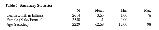
asdoc sum wealthworthinbillions female age, ///
    save(example) label ///
    title(Table 1: Summary Statistics) ///
    dec(2) ///
    statistics(N mean min max) ///
    replace
Here’s what the table will look like in your word document:
Correlation tables & appending to one document with asdoc
You can also create correlation tables. I’m also using this as an example to show you how to “append” a new table to the same document you created before. Both commands are relatively simple.
For correlation tables just add your asdoc command to the beginning of the line.
To append, or paste, the new table to the document you put the last document you created, just add append after the comma.
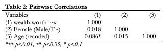
asdoc pwcorr wealthworthinbillions female age, star(0.05) ///
        append ///
        label ///
        title(Table 2: Pairwise Correlations)
Here’s what the table will look like in your word document:
Putting categorical variables in an asdoc descriptive table
One of the frustrating things about asdoc is that it doesn’t let you display the summary statistics for categorical variables. There are two possible solutions we will look at.
Option 1: Show as frequency tables
Here you just add asdoc prior to your tabulate command.
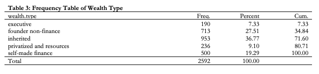
asdoc tab wealthtype2, save(example) ///
            append ///
            title(Table 3: Frequency Table of Wealth Type)
Here’s what the table will look like in your word document:
Option 2: Create a series of binary variables
First create a series of binary variables from your categorical variable. Here we’ll use wealthtype as an example.
tab wealthtype2, gen(wealthtype_)
            label var wealthtype_1 "Wealth Type: Executive"
            label var wealthtype_2 "Wealth Type: Founder Non-Finance"
            label var wealthtype_3 "Wealth Type: Inherited"
            label var wealthtype_4 "Wealth Type: Privatized and Resources"
            label var wealthtype_5 "Wealth Type: Self-Made Finance"
wealth.type | Freq. Percent Cum.
-------------------------+-----------------------------------
executive | 190 7.33 7.33
founder non-finance | 713 27.51 34.84
inherited | 953 36.77 71.60
privatized and resources | 236 9.10 80.71
self-made finance | 500 19.29 100.00
-------------------------+-----------------------------------
Total | 2,592 100.00
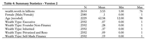
Then we can include all of those binary (aka indicator) variables in the summarize command with asdoc at the front. Note: the asterics after wealthtype_ tells Stata to include ALL variables that begin with that string.
asdoc sum wealthworthinbillions female age wealthtype_*, ///
            save(example) ///
            append ///
            label   ///
            title(Table 4: Summary Statistics - Version 2) ///
            dec(2) ///
            statistics(N mean min max)
Here’s what the table will look like in your word document:
Regression tables with asdoc
Now we can move to creating regression tables with asdoc. Again, we just have to put the asdoc command at the beginning of our regression line, and include any adjustments to the table after a comma.
asdoc regress wealthworthinbillions female age, ///
    save(example) ///
    append  ///
    label ///
    title(Table 5: Wide Regression Model of Wealth Worth) ///
    dec(2) ///
    statistics(N r2) ///
    rep(t) ///
    cnames(Model A)
Here are the additional options we can add:
rep(t)reports t-statistic instead of standard errors (default)cnames(xxxx)names the model in each columnnest: turns the table from “wide” to “long,” which ends up looking more like a traditional results table similar toesttab
Here is the example with nest:
asdoc regress wealthworthinbillions female age, ///
    save(regression) replace ///
    label ///
    title(Table 6: Nested Regression Model of Wealth Worth) ///
    dec(2) ///
    statistics(N r2) ///
    rep(t) ///
    cnames(Model A) ///
    nest
And once you’ve created that first table, you can add additional models to the same table using append:
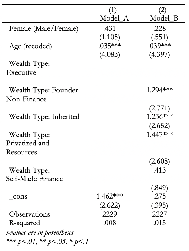
asdoc regress wealthworthinbillions female age wealthtype_*, ///
        label ///
        nest ///
        append ///
        cnames(Model B)
Here’s what the final table should look like:
10.4 Challenge Activity
Look back at your last homework assignment. If you did not use one of these commands to create your regression tables, try to store your models and create a nested regression table.