19 Lab 9 (R)

19.1 Lab Goals & Instructions

Goals

Use dfbetas to identify extreme observations
Use a joint test to test significance of groups of variables

Instructions

Today’s lab you will be following along live. If you’d like to try out the examples on your own, I’ve included the incomplete and complete script files from today’s examples.

Libraries

library(tidyverse)
library(car)

Jump Links to Commands in this Lab:

dfbeta
joint test

Lab Files

Download UM_DEIStudentSurvey.rda

Download 401-1-Lab9.R

19.2 Outliners with DFBETA

Outliers are observations that are far outside of the pattern of observations for other cases. Some outliers will influence your model more than others. Our goal is to understand if there are outlier observations in our model so we can decide what to do with them.

Just like extreme observations can skew our mean, an outlier or two can change our results.

DFBETA: assesses how much each observation affects the regression. It assesses this by calculating how the slope changes when that observation is deleted. If the absolute value of DFBETA is greater than 2 / sqrt(n) OR 1 then you should consider dropping that observation.

STEP 1: Run the regression

fit1 <- lm(satisfaction ~ climate_gen + climate_dei + undergrad + female +
              race_5, data = df_umdei)

STEP 2: Calculate DFBETA
This command creates a dfbeta variable for each variable in your regression. So the column for dfbeta_1: climate_gen will let you know what the change in slope would be if that value of climate_gen were removed from the regression.

dfbetas <- as.data.frame(dfbetas(fit1))
head(dfbetas)

Table 19.1:
(Intercept)	climate_gen	climate_dei	undergrad	female	race_5Black	race_5Hispanic/Latino	race_5Other	race_5White
0.00849	0.00381	-0.00962	-0.0108	-0.0112	-0.000414	0.000792	-0.000175	0.0105
-0.0398	-0.00702	0.0421	0.0143	0.0298	0.00793	0.0429	0.00356	-0.00238
-0.0271	0.0113	0.00998	0.0192	0.0182	0.0473	0.000168	0.00189	-0.00214
0.00954	0.00925	-0.0193	-0.0262	0.0222	-0.00447	-0.000249	0.0681	0.00274
-0.0602	-0.00925	-0.045	0.0945	0.0787	0.128	0.154	0.133	0.191
-0.00394	0.000652	0.00511	-0.00564	-0.00606	0.00268	0.00152	0.00121	-0.00614

STEP 3: See your threshold number

thresh <- 2 / sqrt(1434)
thresh

[1] 0.05281477

We are for any values over 0.05 or lower than -0.05

STEP 4: Visualize the DFBETAS
We are going to use base R to make some quick plots.

plot(dfbetas$climate_gen, type='h')
  abline(h = thresh, lty = 2)
  abline(h = -thresh, lty = 2)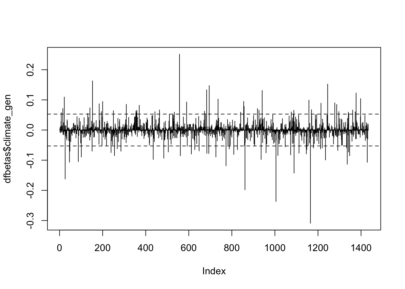

So many observations above the 0.05 threshold! Because that threshold is not particularly helpful, we’ll use 1 as the threshold, which is also pretty common.

plot(dfbetas$climate_gen, type='h')
  abline(h = 1, lty = 1)
  abline(h = -1, lty = 1)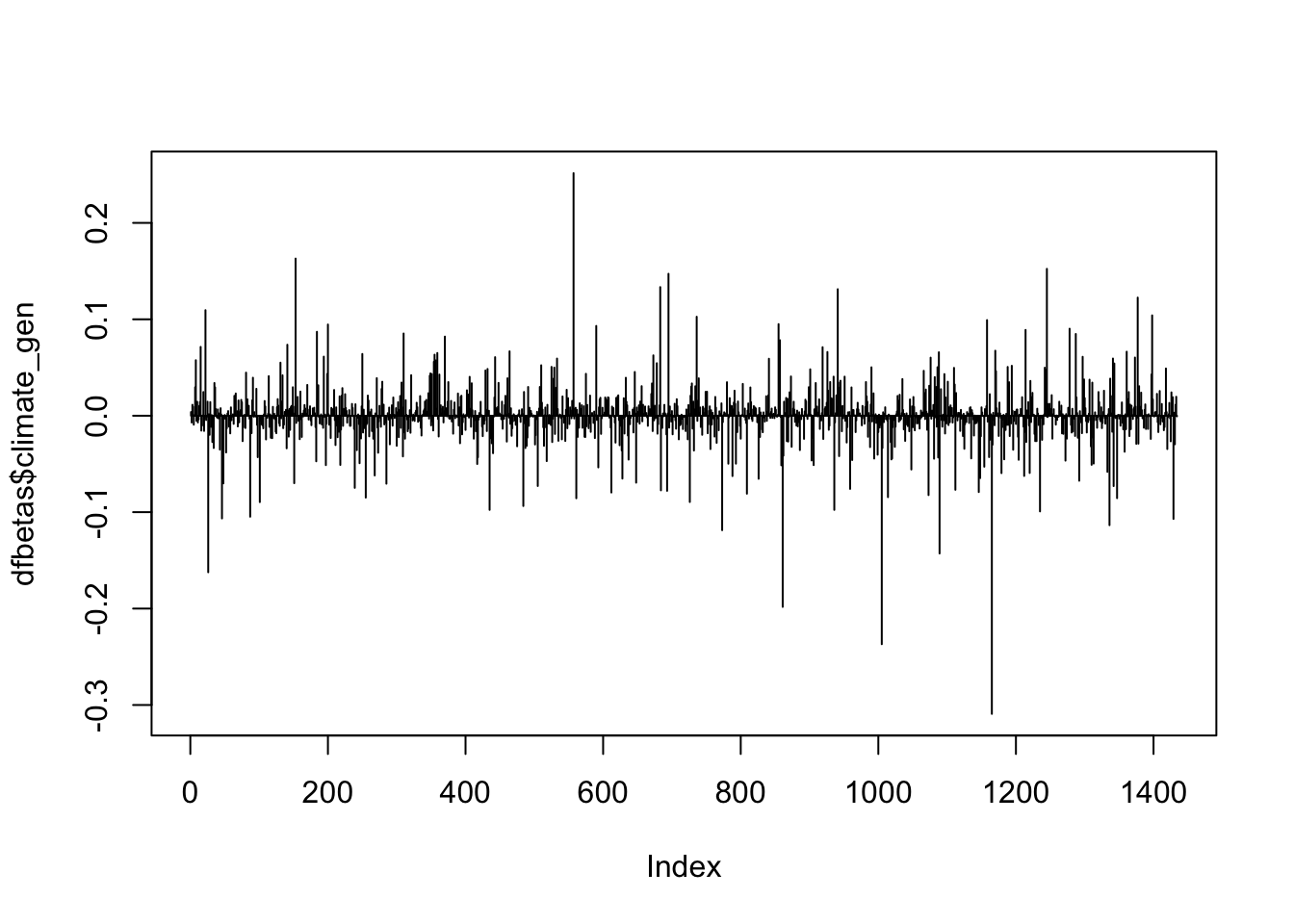

In each plot, the x-axis displays the index of each observation in the dataset and the y-value displays the corresponding DFBETAS for each observation and each predictor.

STEP 5: Locate the observations that are influential
List the index of the observations that are above our threshold of influence for climate_gen.

Note I am showing observations between (.05 and 100) in the first command and (1 and 100 in the second). I added an arbitrary cap at a high number to avoid having Stata list the missing values, which would show up because Stata understands them as infinity in logical statements.

# At the 2 / sqrt(n) threshold
dfbetas %>%
    filter( . > thresh)

# At the 1 threshold
dfbetas %>%
  filter( . > 1)

I’m not showing the results here because they would be too long. Run the script file to see the output!

19.3 Outliers with Cooks Distance

You’ll remember that R has some great built in plots after a regression. It produces one that shows all observations beyond Cook’s distance. Where dfbeta measures how the slow changes, Cook’s Distance measures how the predicted values change when an observation is removed. There is only one Cook’s Distance value per observation.

The threshold for Cook’s Distance is generally \(3 * mean(cooks distance values)\)

On this diagnostic plot, any point that falls outside of Cook’s distance (the red dashed lines) is considered to be an influential observation.

plot(fit1, which = 5)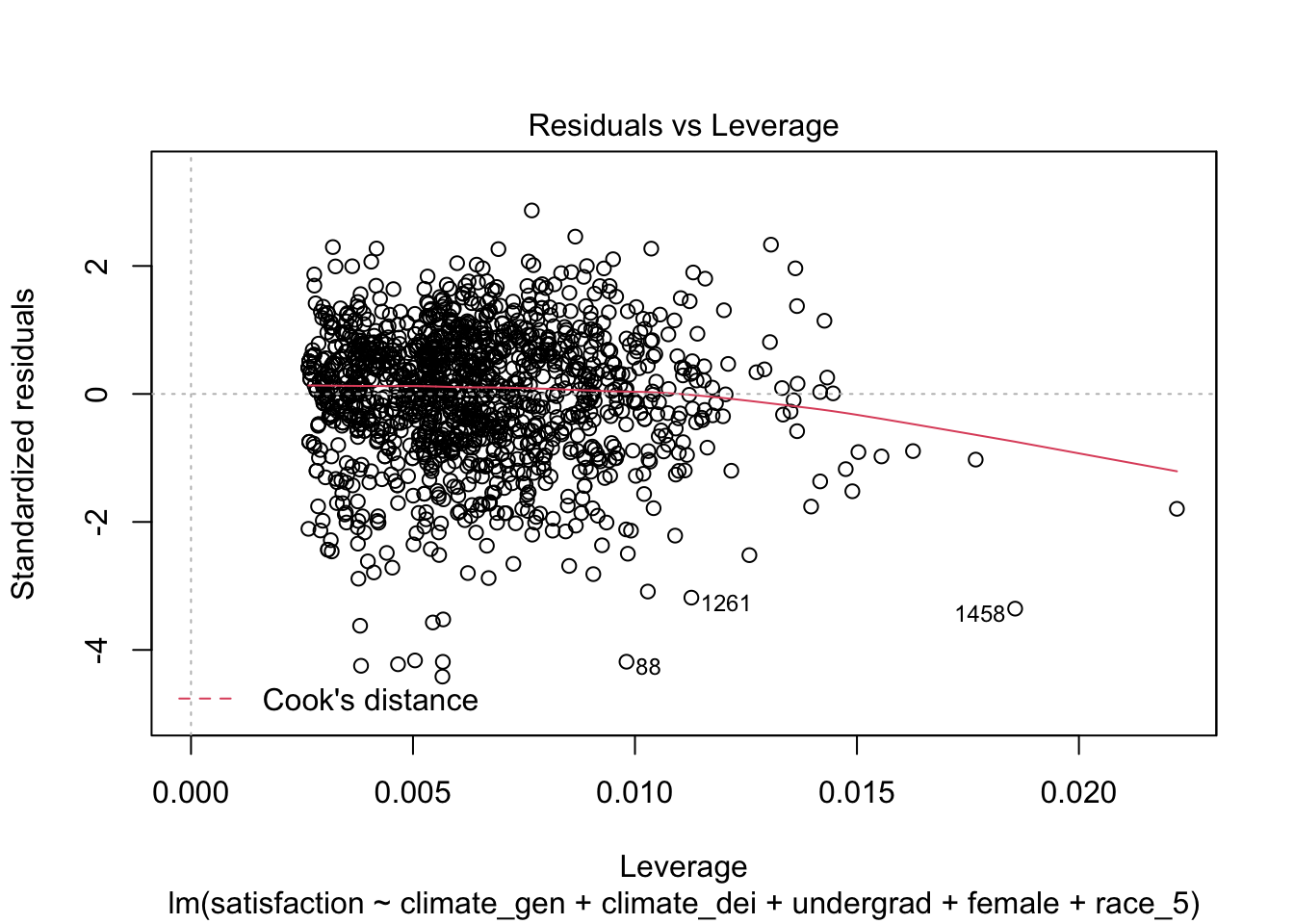

No outliers according to Cook’s Distance!

You can also look at this plot, which plots each Cook’s Distance as a line. The threshold isn’t even shown here because all the values are under the threshold.

plot(fit1, which = 4)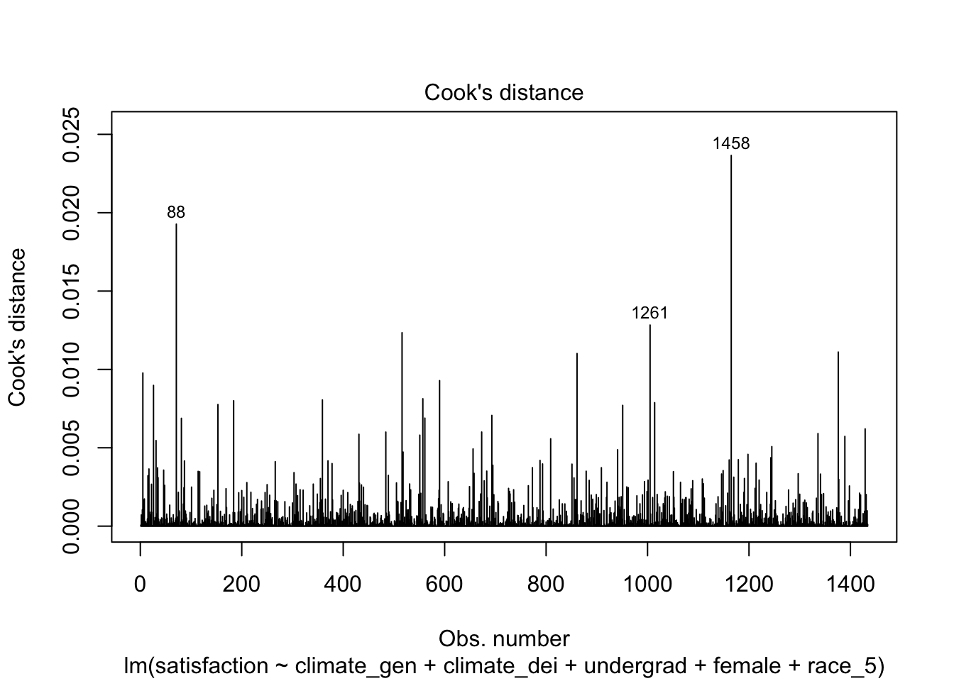

19.4 Joint Tests

Sometimes, you might want to carry out a joint test of coefficients. This is particularly important if you are concerned about bias within your model/a multicollinearity you are worried you can’t/don’t want to solve.

summary(fit1)


Call:
lm(formula = satisfaction ~ climate_gen + climate_dei + undergrad + 
    female + race_5, data = df_umdei)

Residuals:
    Min      1Q  Median      3Q     Max 
-3.5053 -0.4270  0.0845  0.5260  2.2735 

Coefficients:
                      Estimate Std. Error t value Pr(>|t|)    
(Intercept)            0.59359    0.13906   4.269 2.10e-05 ***
climate_gen            0.56052    0.03842  14.589  < 2e-16 ***
climate_dei            0.29779    0.03521   8.458  < 2e-16 ***
undergrad              0.03675    0.04395   0.836   0.4031    
female                -0.10163    0.04353  -2.335   0.0197 *  
race_5Black           -0.45946    0.07830  -5.868 5.48e-09 ***
race_5Hispanic/Latino -0.04658    0.07090  -0.657   0.5113    
race_5Other           -0.05166    0.08383  -0.616   0.5379    
race_5White            0.07266    0.05885   1.235   0.2172    
---
Signif. codes:  0 '***' 0.001 '**' 0.01 '*' 0.05 '.' 0.1 ' ' 1

Residual standard error: 0.7959 on 1425 degrees of freedom
  (366 observations deleted due to missingness)
Multiple R-squared:  0.415, Adjusted R-squared:  0.4118 
F-statistic: 126.4 on 8 and 1425 DF,  p-value: < 2.2e-16

To test whether climate_gen and climate_dei together equal have a significant effect in the model we use linearHypothesis() from the car package

linearHypothesis(fit1, c("climate_gen = 0", "climate_dei = 0"))

Table 19.2:
Res.Df	RSS	Df	Sum of Sq	F	Pr(>F)
1.43e+03	1.36e+03
1.42e+03	903	2	453	357	1.57e-126

The hypothesis test here is that these two coefficients TOGETHER have a value of 0. The fact that we have a p-value < 0.05 means we reject the hypothesis and find that AT LEAST ONE OF THESE VARIABLES HAS A RELATIONSHIP GREATER THAN 0.

BONUS
Though we don’t cover this in class, you can also use the ‘test’ command to find out if two variables are equal to each other. This is especially useful if your question is related to: whether theory 1 (var1) has a significiantly different effect from theory 2 (var2).

For example: I’m interested in which of these (general climate / dei climate) has a greater effect on student satisfaction. I can use test to see if their coefficients are equal (if var1-var2 = 0),

linearHypothesis(fit1, "climate_gen = climate_dei")

Table 19.3:
Res.Df	RSS	Df	Sum of Sq	F	Pr(>F)
1.43e+03	913
1.42e+03	903	1	9.94	15.7	7.83e-05

You might think: how do I interpret this? The null hypothesis here is that the two coefficients are EQUAL to each other. Since p-value<0.5, we reject the null hypothesis, telling us the two variables are statistically different from each other. Given what our results shows us, we can then see that the difference is that general climate has a greater effect on satisfaction for students than dei climate.