2 Lab 1 (Stata)
2.1 Lab Goals & Instructions
- Review the basics of data cleaning in Stata
- Learn the importance of annotating code
- Start develop your own coding style
Instructions
- Download the data file (
SOC401_W21_Billionaires.dta) and .do script (401-1-Lab1.do) from the links below. - Create a file structure following the instructions in 2.3 below
- Work through the .do script, executing each line of code. This page contains the same material, with more explanation about the commands used.
- Read through the Importance of Annotation and Clean Code, and complete the short activity at the bottom of the page. Email the .do script file to me by class on Monday.
Jump Links to Commands in this Lab:
cd (set working directory)
use (load stata files)
import delimited (load .csv)
describe
mdesc for missing data
summarize
tabulate
generate
recode
replace
histogram
graph box (box plot)
graph bar (bar plot)
keep
drop
save
export delimited
2.3 Create a File Structure
Life can get messy and so can data analysis. Creating a file structure is the equivalent of keeping a clean work space. You may not mind a messy desk, but a messy file structure will be a nightmare for your collaborators and increase your risk of making mistakes in your analysis. With quantitative data analysis, file management is crucial. I am going to suggest a file structure that you follow in this class. It will ensure that the relative pathways I include in lab script files will run.
For your first task, create the following file structure for this class.
- Decide where on your computer you’d like to store class files. Create a new folder in that spot titled anything you like. Example: 401_Linear_Regression. DO NOT include spaces in your folder title.
- Create the following sub-folders in your main folder:
- data_raw
- data_work
- scripts
- figs_output
- Move
SOC401_W21_Billionaires.dtato yourdata_rawfolder. - Move
401-1-Lab1.doto yourscriptsfolder.
When you begin labs, you should move all raw data files and script files to the appropriate locations.
![]() Data Tip
Data Tip
Why do I need two separate folders for data?
You should aways store your original, raw data files in a place where they are in no danger of being saved over, altered, or lost. One great way of protecting your original data files is to create two folders for data: one folder for your raw files and one folder where you can saved cleaned datasets and subsets.
2.4 Data Cleaning
Ninety-five percent of the work of quantitative research is getting your data in shape to run your model. This tutorial assumes that you opened Stata and run a few commands before. If you are have not used Stata before, here are some resources to help you get started coding in Stata.
- Stata Tutorial from Princeton: A great overview of Stata basics
- Stata Tutorial from University of South Australia
- Stata Commands Cheat Sheet
Northwestern’s Research Computing Services offers great trainings in a variety of software languages. They do not have regular trainings in Stata, but you can set up individual meetings to help work through problems in your code. Check them out and get on their email list.
Set up the environment
Working Directory
Before you get to work cleaning your data, you need to let the software know where to grab and save your files. This saves you from having to type in a long file path anytime you want to do something. You must begin any Stata .do file by setting your working directory. Your working directory is the folder on your computer where you want to store all your data and script files. Below you will see the path to my working directory. You should replace the filepath with the one you want to use.
cd "/Users/srwerth/Documents/Work_Research/Regression_Labs"If you are having trouble getting this command to work, make sure there are no spaces in any of the parent folders in your file path.
Do File Set-up
Now that you’ve set your working directory, you can tell Stata to go grab your data and load it into your working environment.
There are a couple lines of code you want to put at the beginning of your .do file to keep your code running smoothly.
clear all: Clears the stata environment before you run your code.capture log close: If there’s a previous log set up, this code closes it.log using Lab1.scl, replace: This creates a new log file, which is a file that tracks all the code you run in the session. This is important for reviewing your analysis after the fact. Rename the file whatever you like for each lab.version 17: This command tells Stata what version of the software you wrote this .do file in, in case you are running it in a different version later. Sometimes commands can change between versions. This prevents any inconsistencies between versions from causing errors.
clear all
capture log close
log using Lab1.smcl, replace
version 17
Load your data
Now you are ready to load your data. Loading data that is in Stata’s data formats is easy. An Stata data file ends in .dta. Note how I get to use a relative path, just telling Stata to look in the data_raw folder, and then the dataset name. This is because we set our working directory!
use "data_raw/SOC401_W21_Billionaires.dta"You can also load data in other formats. A CSV file is one of the most common data formats.
import delimited "data_raw/SOC401_W21_Billionaires.csv"Check out this tutorial on how to load excel data:
https://www.stata.com/manuals/dimportexcel.pdf
Exploring your data
When you begin any new project, it is important to understand the condition of your variables. Here are a few important functions you need to begin that process.
![]() Data Tip
Data Tip
Remember if this script or any other uses a command that you are not familiar with, you can search for the function online or type ‘help’ and then the name of the function you want to look up in the command line. For example, ‘help describe’ will pull up the documentation for that command.
Let’s start by taking a global look at your dataset.
The describe function provides an overview of your dataset. The output includes the number of observations, variables, and a description of each variable in the dataset. The description includes the format and any labels already attached to each variable.
describeContains data from data_raw/SOC401_W21_Billionaires.dta
Observations: 2,614
Variables: 21 9 Jan 2021 15:56
--------------------------------------------------------------------------------
Variable Storage Display Value
name type format label Variable label
--------------------------------------------------------------------------------
name str45 %45s
rank int %8.0g
year int %8.0g
companyfounded int %8.0g company.founded
companyname str59 %59s company.name
demographicsage byte %8.0g demographics.age
locationgdp double %10.0g location.gdp
wealthworthin~s float %9.0g wealth.worth in billions
wealthhowfrom~g str4 %9s wealth.how.from emerging
wealthhowwasf~r str4 %9s wealth.how.was founder
wealthhowwasp~l str4 %9s wealth.how.was political
wealthhowinhe~2 long %24.0g wealthhowinherited2
wealth.how.inherited
wealthhowcate~2 long %18.0g wealthhowcategory2
wealth.how.category
wealthtype2 long %24.0g wealthtype2
wealth.type
wealthhowindu~2 long %31.0g wealthhowindustry2
wealth.how.industry
locationregion2 long %24.0g locationregion2
location.region
locationcount~2 long %8.0g locationcountrycode2
location.country code
locationcitiz~2 long %20.0g locationcitizenship2
location.citizenship
demographicsg~2 long %14.0g demographicsgender2
demographics.gender
companysector2 long %52.0g companysector2
company.sector
companyrelati~2 long %46.0g companyrelationship2
company.relationship
--------------------------------------------------------------------------------
Sorted by: You can also look at a specific variable you want to learn more about
describe demographicsgender2Variable Storage Display Value
name type format label Variable label
--------------------------------------------------------------------------------
demographicsg~2 long %14.0g demographicsgender2
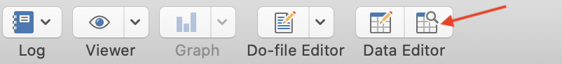
demographics.genderIf you want to look at your data set in a spreadsheet-type format you can look at the Data Editor in browse mode. You can open the Data Editor by clicking on the icon below on the top bar. Make sure you click on the icon with the magnifying glass (browse mode), not the pencil (edit mode). You do not want to accidentally edit your data.
Look at missing observations in your dataset
To look at missing values for each variable in your data set we need to download a new function into Stata. The mdesc function makes looking at missing values easy. To install a Stata program you can run search mdesc in the command line and click the link in the program information to install the program.
ssc install mdescNow you are ready to look at the missing values in your dataset
mdesc Variable | Missing Total Percent Missing
----------------+-----------------------------------------------
name | 0 2,614 0.00
rank | 0 2,614 0.00
year | 0 2,614 0.00
companyfou~d | 0 2,614 0.00
companyname | 38 2,614 1.45
demographi~e | 0 2,614 0.00
locationgdp | 0 2,614 0.00
wealthwort~s | 0 2,614 0.00
wealthhowf~g | 0 2,614 0.00
wealthhoww~r | 0 2,614 0.00
wealthhoww~l | 0 2,614 0.00
wealthhow~d2 | 0 2,614 0.00
wealthhowc~2 | 1 2,614 0.04
wealthtype2 | 22 2,614 0.84
wealthh~try2 | 1 2,614 0.04
locationre~2 | 0 2,614 0.00
locationco~2 | 0 2,614 0.00
locationci~2 | 0 2,614 0.00
demographi~2 | 34 2,614 1.30
companysec~2 | 23 2,614 0.88
companyrel~2 | 46 2,614 1.76
----------------+-----------------------------------------------Or you can look at missing values for a specific variable
mdesc companyname Variable | Missing Total Percent Missing
----------------+-----------------------------------------------
companyname | 38 2,614 1.45
----------------+-----------------------------------------------Descriptive statistics for continous variables using summarize
You can generate simple descriptive statistics (mean, standard deviation, range, etc.) with the summarize command. Looking at descriptive statistics is not only helpful to get a sense of your data, they can also be helpful checks as you work on cleaning a dataset.
summarize demographicsage Variable | Obs Mean Std. dev. Min Max
-------------+---------------------------------------------------------
demographi~e | 2,614 53.34124 25.33332 -42 98If you add , detail to the command you can see additional descriptive statistics,
including skew, variance and quartiles.
summarize demographicsage, detail demographics.age
-------------------------------------------------------------
Percentiles Smallest
1% 0 -42
5% 0 -7
10% 0 0 Obs 2,614
25% 47 0 Sum of wgt. 2,614
50% 59 Mean 53.34124
Largest Std. dev. 25.33332
75% 70 95
90% 79 96 Variance 641.7771
95% 84 96 Skewness -1.104472
99% 90 98 Kurtosis 3.330685Frequency tables for categorical variables using tabulate
Tabulate produces a frequency table showing how many observations there are for each value.
tabulate demographicsgender2demographics.g |
ender | Freq. Percent Cum.
---------------+-----------------------------------
female | 249 9.65 9.65
male | 2,328 90.23 99.88
married couple | 3 0.12 100.00
---------------+-----------------------------------
Total | 2,580 100.00If you add , nolabel it shows you the values without their label. This is how the values appear in the actual data, which is important to know when you have to recode your data. With this example, you can see that female is coded as 1, male is coded as 2, and married couple is coded as 3.
tabulate demographicsgender2, nolabeldemographic |
s.gender | Freq. Percent Cum.
------------+-----------------------------------
1 | 249 9.65 9.65
2 | 2,328 90.23 99.88
3 | 3 0.12 100.00
------------+-----------------------------------
Total | 2,580 100.00If you add , missing it will add a row to the table showing the number of missing values for that variable.
tabulate demographicsgender2, missingdemographics.g |
ender | Freq. Percent Cum.
---------------+-----------------------------------
female | 249 9.53 9.53
male | 2,328 89.06 98.58
married couple | 3 0.11 98.70
. | 34 1.30 100.00
---------------+-----------------------------------
Total | 2,614 100.00Note: you can also shorten tabulate to tab and the function will run the same.
Cleaning variables
In the previous section, we learn the code to check the state of a variable when we first open the dataset. Most of the time, you’re likely to find that the variable isn’t ideal to work with. It is important to learn these commands to make a variable ready for your use.
Let’s take a closer look at the variable for gender again:
tabulate demographicsgender2demographics.g |
ender | Freq. Percent Cum.
---------------+-----------------------------------
female | 249 9.65 9.65
male | 2,328 90.23 99.88
married couple | 3 0.12 100.00
---------------+-----------------------------------
Total | 2,580 100.00I notice a few things you will want to change about that variable:
- The variable name is tedious to type
- We want this to be a dummy variable where 1 is female and 0 is not female (in this binary, male).
- We have three married couples in our data set coded as 3
Let’s create a new variable with a better name and recode it how you’d like it.
generate to create new variables
If you want to label the 3 married couples as 0, aka not female, take the following steps. First let’s generate a new variable female with the same values as demographicsgender2. We’ll also go ahead and label that variable “Female.” Note that I’ve shortened generate to gen and it works the same.
gen female = demographicsgender2
label variable female "Female (recoded)"
To breakdown the line of code to label: the command is label variable, the variable you are labeling is female, and the label is “Female (recoded).”
recode to transform the values of a variable
Now let’s take our new variable and recode the values so that 0 means “Not Female” and 1 means “Female.” In this example, we’re taking all the married couples and labeling them as 0. In this code you are telling Stata to recode the variable female so that a 3 becomes a 0, a 2 becomes a 0 and a 1 stays a 1.
recode female (3 = 0) (2 = 0) (1 = 1) You should also at this point apply a label to these new values, so your tables and graphs will be easier to read. This is a two step process. First you create an object that stores the labels you want to apply to each value. label define is the command and gender is the name of the object you are creating.
label define gender 0 "Not Female" 1 "Female"Second, you apply that label object to the variable. label values is the command, female is the name of the variable you want to label, and gender is the label object you want to apply to it.
label values female genderLet’s run a crosstab table to make sure that everything came out right. Looks like everything landed where it is supposed to.
tab female demographicsgender2 Female | demographics.gender
(recoded) | female male married c | Total
-----------+---------------------------------+----------
Not Female | 0 2,328 3 | 2,331
Female | 249 0 0 | 249
-----------+---------------------------------+----------
Total | 249 2,328 3 | 2,580 replace to transform the values of a variable
There’s another way to recode variables. Both options work just as well, so it is truly your preference which one you want to use. We’ll practice using the replace command by recoding our gender variable a different way. Let’s make a new variable so 0 only refers to “Male” and 1 only refers to “Female.” You will recode the married couples to missing.
First, you will generate a new variable, female2. In this instance we set all the values of the new variable to missing. We’ll also label it.
gen female2 = .
label variable female2 "Female (Male/Female)"
Now let’s recode our values using the replace command. This command replaces the values of your variable, based on the values of another variable. Here you are telling Stata to replace the value of female2 if demographicsgender2 is equal to 2. On the second line you make the value of female2 1 if demographicsgender is equal to 1.
replace female2 = 0 if demographicsgender2 == 2
replace female2 = 1 if demographicsgender2 == 1
Let’s label it as well
label define gender2 0 "Male" 1 "Female"
label values female2 gender2
Because you set all the values to missing and do not recode the 3 values to anything, they will remain missing. Let’s double check with our crosstab using tabulate. We’ll add , missing to see if the 3 values were recoded correctly (and everything looks good).
tab female2 demographicsgender2, missing Female |
(Male/Fema | demographics.gender
le) | female male married c . | Total
-----------+--------------------------------------------+----------
Male | 0 2,328 0 0 | 2,328
Female | 249 0 0 0 | 249
. | 0 0 3 34 | 37
-----------+--------------------------------------------+----------
Total | 249 2,328 3 34 | 2,614 Note: In Stata when you are creating something new, as with the generate command, you use a single equals sign. Your new variable female should equal what follows. When you’re writing a test statement referring to something that already exists, you use double equals sign (==), as we do in the second part of the replace command. .
Now let’s try another example, looking at the variable for age:
tab demographicsage, missingdemographic |
s.age | Freq. Percent Cum.
------------+-----------------------------------
-42 | 1 0.04 0.04
-7 | 1 0.04 0.08
0 | 383 14.65 14.73
12 | 1 0.04 14.77
21 | 1 0.04 14.80
24 | 2 0.08 14.88
28 | 2 0.08 14.96
29 | 4 0.15 15.11
30 | 4 0.15 15.26
31 | 5 0.19 15.46
32 | 4 0.15 15.61
33 | 8 0.31 15.91
34 | 6 0.23 16.14
35 | 8 0.31 16.45
36 | 7 0.27 16.72
37 | 8 0.31 17.02
38 | 7 0.27 17.29
39 | 10 0.38 17.67
40 | 13 0.50 18.17
41 | 15 0.57 18.75
42 | 18 0.69 19.43
43 | 19 0.73 20.16
44 | 25 0.96 21.12
45 | 29 1.11 22.23
46 | 42 1.61 23.83
47 | 35 1.34 25.17
48 | 46 1.76 26.93
49 | 57 2.18 29.11
50 | 65 2.49 31.60
51 | 42 1.61 33.21
52 | 54 2.07 35.27
53 | 44 1.68 36.95
54 | 47 1.80 38.75
55 | 63 2.41 41.16
56 | 55 2.10 43.27
57 | 60 2.30 45.56
58 | 63 2.41 47.97
59 | 61 2.33 50.31
60 | 76 2.91 53.21
61 | 54 2.07 55.28
62 | 64 2.45 57.73
63 | 61 2.33 60.06
64 | 65 2.49 62.55
65 | 52 1.99 64.54
66 | 56 2.14 66.68
67 | 50 1.91 68.59
68 | 64 2.45 71.04
69 | 65 2.49 73.53
70 | 59 2.26 75.78
71 | 55 2.10 77.89
72 | 59 2.26 80.15
73 | 52 1.99 82.13
74 | 46 1.76 83.89
75 | 36 1.38 85.27
76 | 45 1.72 86.99
77 | 43 1.64 88.64
78 | 30 1.15 89.79
79 | 26 0.99 90.78
80 | 21 0.80 91.58
81 | 28 1.07 92.65
82 | 24 0.92 93.57
83 | 26 0.99 94.57
84 | 20 0.77 95.33
85 | 25 0.96 96.29
86 | 21 0.80 97.09
87 | 18 0.69 97.78
88 | 17 0.65 98.43
89 | 7 0.27 98.70
90 | 12 0.46 99.16
91 | 4 0.15 99.31
92 | 6 0.23 99.54
93 | 4 0.15 99.69
94 | 3 0.11 99.81
95 | 2 0.08 99.89
96 | 2 0.08 99.96
98 | 1 0.04 100.00
------------+-----------------------------------
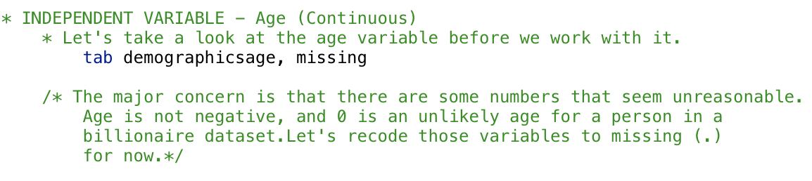
Total | 2,614 100.00The major concern is that there are some numbers that seem unreasonable. Age is not negative, and 0 is an unlikely age for a person in a billionaire dataset. Let’s recode those variables to missing (.) for now. First we generate a new variable named something simpler and easier to type and label it.
generate age = demographicsage
label variable age "Age (recoded)"
Now you’ll use recode to set any values 0 or below to missing.
replace age = . if age <= 0Use summarize to check the new range.
summarize age Variable | Obs Mean Std. dev. Min Max
-------------+---------------------------------------------------------
age | 2,229 62.57649 13.13472 12 98Use mdesc to check the new number of missing values. 385 is equal to all the previous 0, -7, and -42 values.
mdesc age Variable | Missing Total Percent Missing
----------------+-----------------------------------------------
age | 385 2,614 14.73
----------------+-----------------------------------------------![]() Data Tip
Data Tip
Why create a new variable when recoding?
If you have a sharp eye, you’ll notice that we created a new variable rather than changing the name of our original variable and recoding it. Data cleaning is an iterative process. You may make mistakes (you will probably make mistakes) or you may change your mind about how to recode a variable. In each case, having the original variable on hand is always helpful. To preserve your original variable, you create a new variable rather than writing over the old one.
Vizualizing variables
Continuous Variables
While frequency tables and descriptive statistics are helpful, visualizing variables can be helpful to get a look at the shape of our data. For continuous variables or discrete variables with a wide range of values histograms or box plots the go to.
Histograms
histogram age 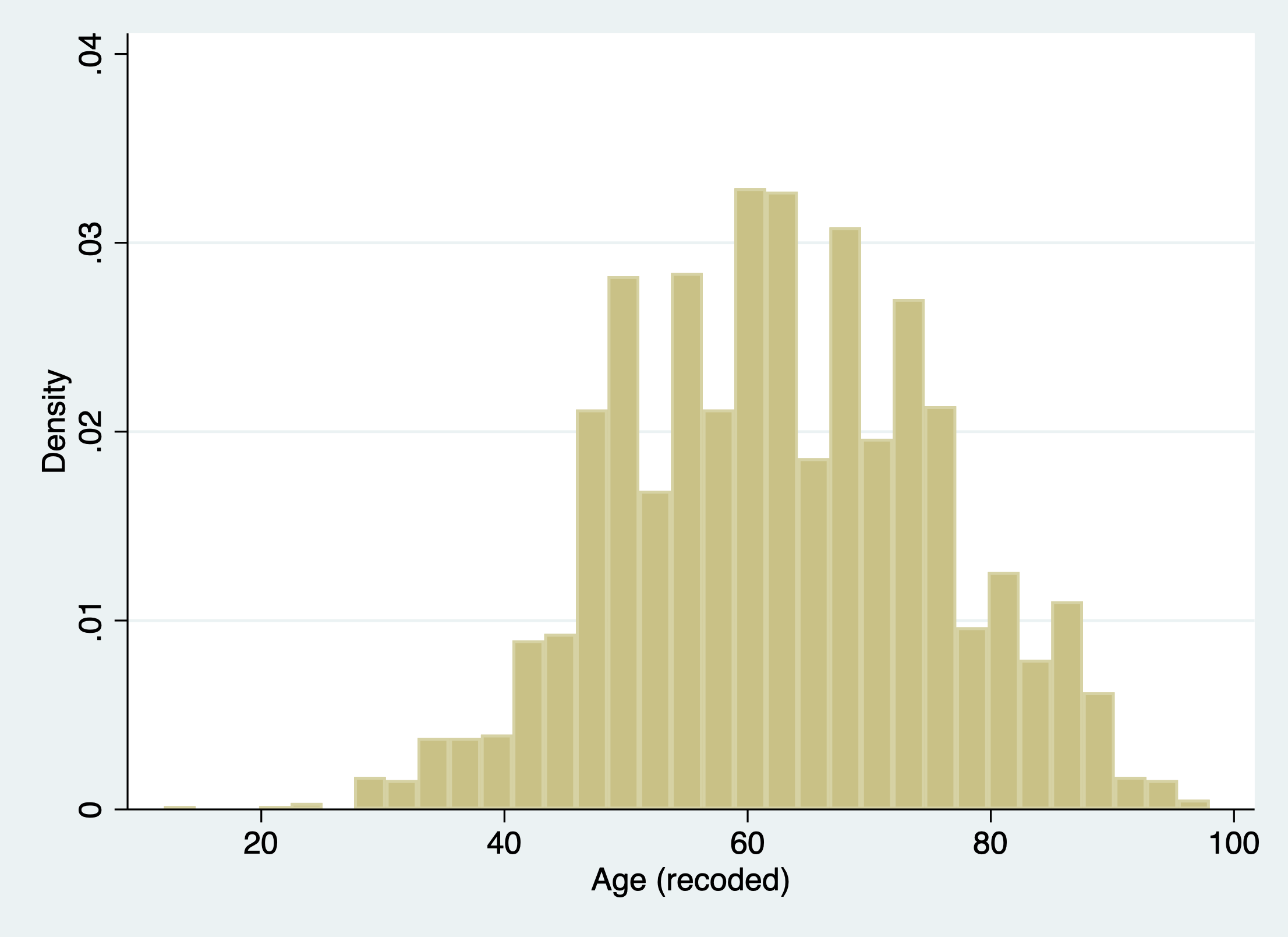
If you want to change the number of bins (i.e. bars),
histogram age, bins(10)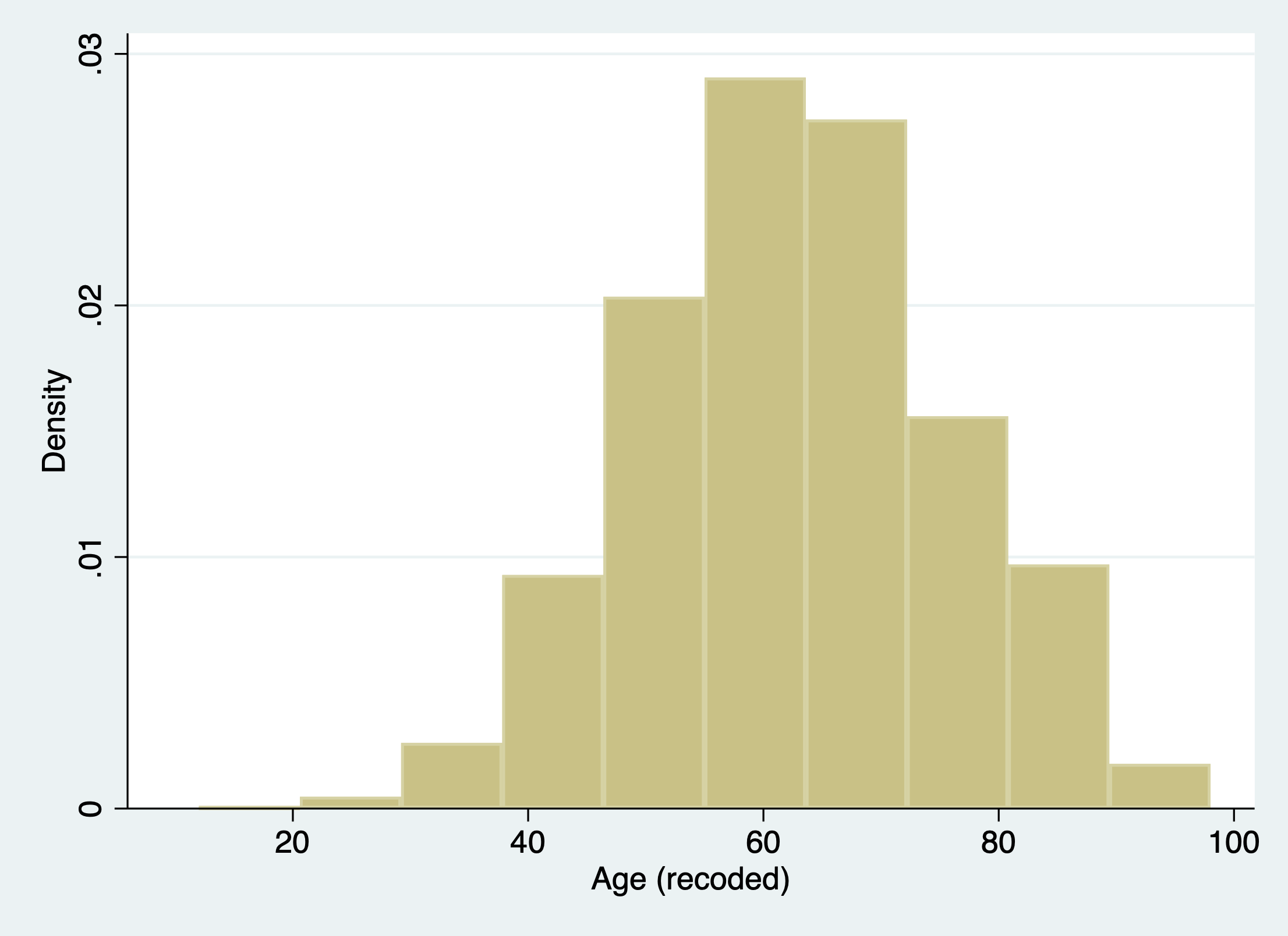
Box plots
Let’s try making a boxplot of age.
graph box age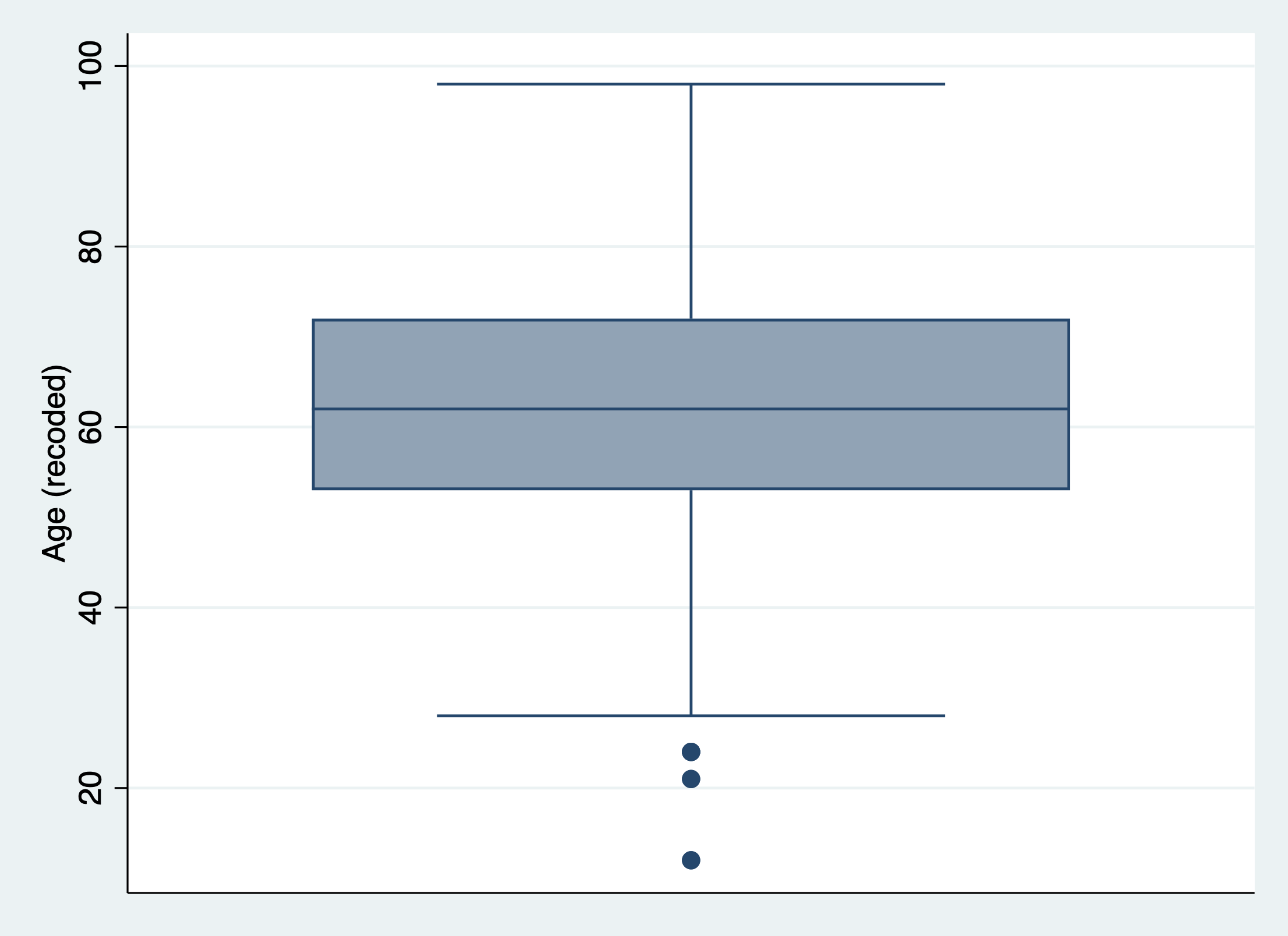
Let’s try making a boxplot of age by gender.
graph box age, over(female2)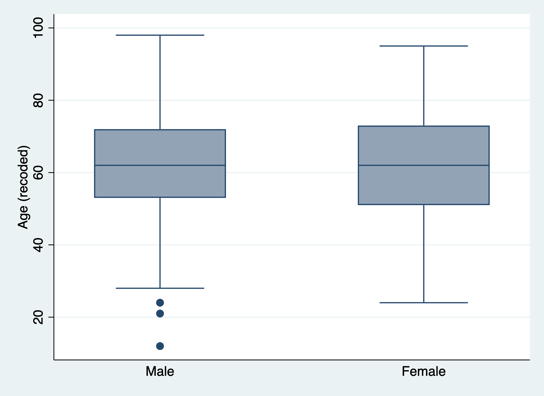
Categorical Variables
Again frequency tables are great, but sometimes a visualization of a categorical data can better communicate patterns. You can get creative, but the easiest option is a simple bar plot.
Bar plots
For the bar plot command, put the variable you want to display in the parentheses in the over() piece of the command. It splits the count over the categories of the variable you specify.
graph bar, over (female)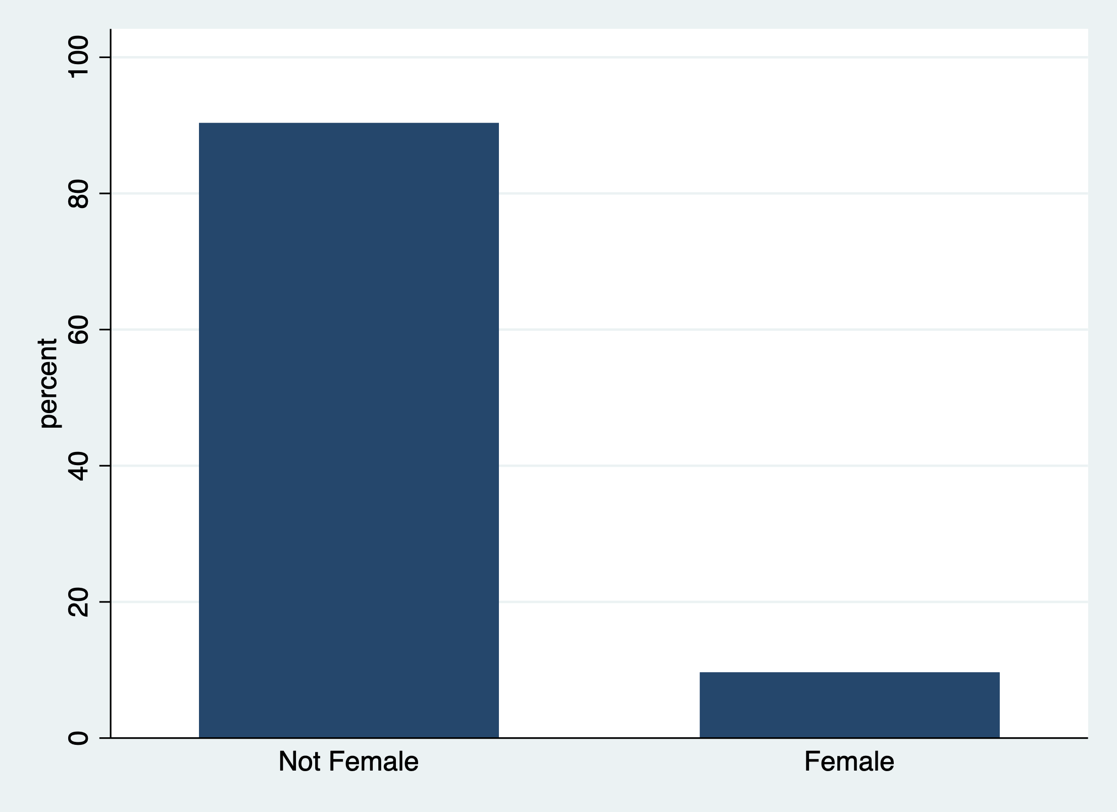
Subsetting and saving data
Sometimes you’ll be working with a huge dataset, and it is easier and cleaner to save a portion of observations and/or variables in a new dataset. This is called a subset.
Subset your data to specific variables
Let’s say you only want to keep the following three variables: year and the two variables you just created: age and female. For this task, you can use the keep command. We’ll check it with the describe command.
keep year age female2
describe
Contains data from data_raw/SOC401_W21_Billionaires.dta
Observations: 2,614
Variables: 3 9 Jan 2021 15:56
--------------------------------------------------------------------------------
Variable Storage Display Value
name type format label Variable label
--------------------------------------------------------------------------------
year int %8.0g
female2 float %9.0g gender2 Female (Male/Female)
age float %9.0g Age (recoded)
--------------------------------------------------------------------------------
Sorted by:
Note: Dataset has changed since last saved.You can also use the drop command if you only want to exclude a variable or two.
drop female2Subset your data to specific observations
But what if you wanted to subset the data to only billionaires 30 or older? For this you can also use the drop command with an if conditional statement added. We’ll check it with summarize.
drop if age < 30
summarize age
(10 observations deleted)
Variable | Obs Mean Std. dev. Min Max
-------------+---------------------------------------------------------
age | 2,219 62.74448 12.91838 30 98Saving your subset
Now that you have your subset, you’ll want to save it. Saving in Stata’s data format is simple. You add the , replace for when you are rurunning this .do file. If there is already a dataset named mysubset.dta, then Stata will save over it with your new changes. Take care with saving over datasets. The action cannot be undone.
save "data_work/mysubset.dta", replaceThere are extra steps to save it other formats. .CSV files, are one of the most common formats you’ll receive and save data in outside of Stata.
export delimited using data_work/mysubset.csv, replace Remember, every time you run these command it writes over your previous save. So be careful about version control and ALWAYS maintain the raw data file in a separate location.
2.5 The Importance of Annotation and Clean Code
A do file (aka a script) is not just a functional document where you conduct your analysis. It is also an important record of your analysis. When you read back through your do files you should be able to understand what each step of code is doing and why. Well-written code scripts:
- Have a header with your name and a title or a short description of what the script contains (e.g., “Cleaning data for regression analysis on billionaires”)
- Document the analytic decisions made about cleaning and analysis
- Can be run from start to finish without errors
You may think that you will remember what you were thinking when you wrote a script, but sometimes you’ll have to step away from an analysis for weeks or months. When you come back to it, your notes will remind you exactly why you coded things the way you did. Your code scripts will also be read by other people. It may be collaborators, advisers, or colleagues who agree to quality check your code to look for errors. It is also more and more common for journals to ask scholars to post their coding files so that other people can replicate your analysis.
How to make notes in your script
The main way to make a note in an Stata .do script is to use the * at the beginning of a line.
Let’s return to our code to subset our data to billionaires 30 or older. In this code I note above the command what it is about to do. In the second command, I include a note one the same line to remind myself that I want to check to make sure the code I ran worked correctly.

You can also use /* */ to create notes that span across multiple lines. For example:
 If you want to add a note to the end of a command you can put a double slash
 //

Tips for Neat Code
Notes are a huge part of making your code readable to yourself and others. However, writing neat code is also an enormous gift you can give to yourself, to the TA grading your do files, and anyone else trying to make sense of your code. Here are my top tips for writing neat code in Stata:
- Split long functions and commands across multiple lines
- Leave spaces around equals signs and other operators
- Create headers and sections in your code
- Create clear names for your variables
Split long functions and commands across multiple lines
Nothing, I repeat, nothing makes code harder to read than shoving it all into one long line. It can be a little tricky to split some commands across multiple lines in Stata, but it is possible and makes your code much cleaner. You can do so by adding a triple forward slash to the end of a line (///). This tells Stata that the command continues on the next line. You can use this over as many lines as you want.
Take this example. Say we wanted to keep many variables in our subset.
keep wealthworthinbillions demographicsage demographicsgender2 wealthhowinherited2 wealthtype2 wealthhowcategory2 locationregion2These lines of code will run just fine, but they are difficult for your eye to parse when squished together. Let your code breathe!
keep wealthworthinbillions demographicsage demographicsgender2 ///
  wealthhowinherited2 wealthtype2 wealthhowcategory2 locationregion2
As a rule, don’t let any line get past about 80 characters. Stata .do files include a vertical line at about this point. I recommend that you don’t write past it in your code scripts. It will help you and the reader avoid the annoying horizontal scroll bar.
Leave spaces around operators
This is another tip to let your code breathe! When coding it is best practice to put a space after any comma or logical operator. Take the line of code below:
replace female2=0 if demographicsgender2==2 | demographicsgender2==3
replace female2=1 if demographicsgender2==1
It works, but it’s cluttered and makes it difficult to read. Take a look at this line in a cleaner format:
replace female2 = 0 if demographicsgender2 == 2 | demographicsgender2 == 3
replace female2 = 1 if demographicsgender2 == 1
Notice how I’ve added a space on both sides of the equals signs. This makes it easier to understand and edit your code.
Create headers and sections in your code
You wouldn’t write a paper without any titles or sections, so don’t write your code without titles or sections! Take a look back at the Stata do script for this lab. Notice how I put a section header for setting up your environment, exploring your data, cleaning your data, and so on. Hopefully this made it easier for you to work through the script.
Create clear names for your variables
Everyone has their own preferred naming system for variables and data sets. The golden rule for naming is consistency. For example, if I recode variables I will often add _rc to the end for recode (e.g., age and age_rc). Other tips:
- Make your names explicit, but brief (e.g.,
billionaires_over30.dta) - Don’t include spaces in your file names, it makes file paths difficult
2.6 Activity
For this class, we expect you to write legible, clean code. To kick start this process, I want you to begin develop your own coding style. By class on Monday, email me (rosewerth@u.northwestern.edu) a script file for a hypothetical data cleaning script. The script should include:
- A script header with your name, the date you created the script, and a short description of what the script contains
- Two section headers
- A command to set your working directory to the main folder you created in this lab
- A note telling me what you find easy about coding in Stata and what you find difficult about coding in Stata.
This should be your template for writing clean scripts for the rest of the quarter. Your template can evolve, but I expect all your scripts moving forward to contain title and section headers and clear annotation for each step in your code.