4 Lab 2 (Stata)

4.1 Lab Goals & Instructions

Goals

• Use scatter plots and correlation to assess relationships between two variables
• Run a basic linear regression
• Interpret the results

Research Question: What features are associated with how wealthy a billionaire is?

Instructions

1. Download the data and the .do file from the lab files below.
2. Run through the .do file and reference the explanations on this page if you get stuck.
3. If you have time, complete the challenge activity on your own.

Jump Links to Commands in this Lab:
scatter (scatter plot)
lfit (line of best fit)
loess (lowess line)
correlate
pwcorr
regress

4.2 Lab Files

Download SOC401_W21_Billionaires_v2.dta

Download 401-1-Lab2.do

4.3 Evaluating Associations Between Variables

In this lab you’ll learn a couple ways to look at the relationship or association between two variables before you run a linear regression. In a linear regression, we assume that there is a linear relationship between our independent (x) and dependent (y) variables. To make sure we’re not horribly off base in that assumption, after you clean your data you should check the relationship between x and y. We’ll look at two ways to do this: scatter plots and correlation.

Note: I’m not including the code to set up your .do file environment here, but it is included in the .do file for lab 2.

Scatter Plots

A scatter plot simply plots a pair of numbers: (x, y). Here’s a simple plot of the point (3, 2).

To look at the relationship between our independent and dependent variables, we plot the (x,y) pairings of all our observations.

Let’s look at the relationship between the two variables of interest in our analysis today: age (x) and wealth (y). You’ll produce a basic scatter plot of x and y, which can let you see at a glance whether there is a linear relationship between the two.

scatter wealthworthinbillions age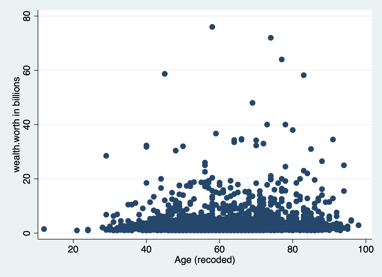

It’s pretty difficult to see a pattern here.

At times, we need extra help to see linear associations. This is especially true whether there are a ton of observations in our data. There may be an association, our eyes just cannot detect it through all the mess. To solve this problem, we add what’s called a line of best fit (aka a linear regression line) over our graph.

Line of Best Fit

When we run a regression, we are generating a linear formula (something like y = ax + b). We can plot that line to visually see the relationship between two variables. In Stata, you do this by using lfit and add it to the end of your scatter plot command. In the lfit command you include the same variables on your scatterplot in the same order.

scatter wealthworthinbillions age || lfit wealthworthinbillions age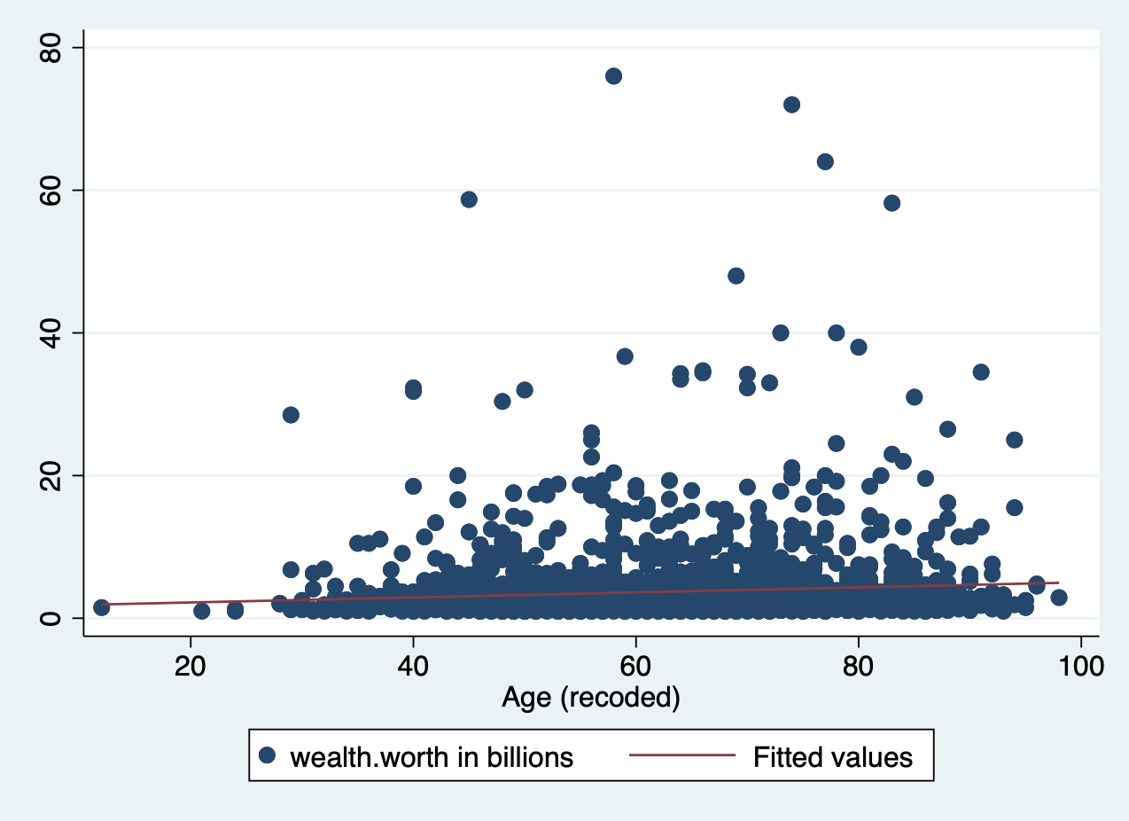

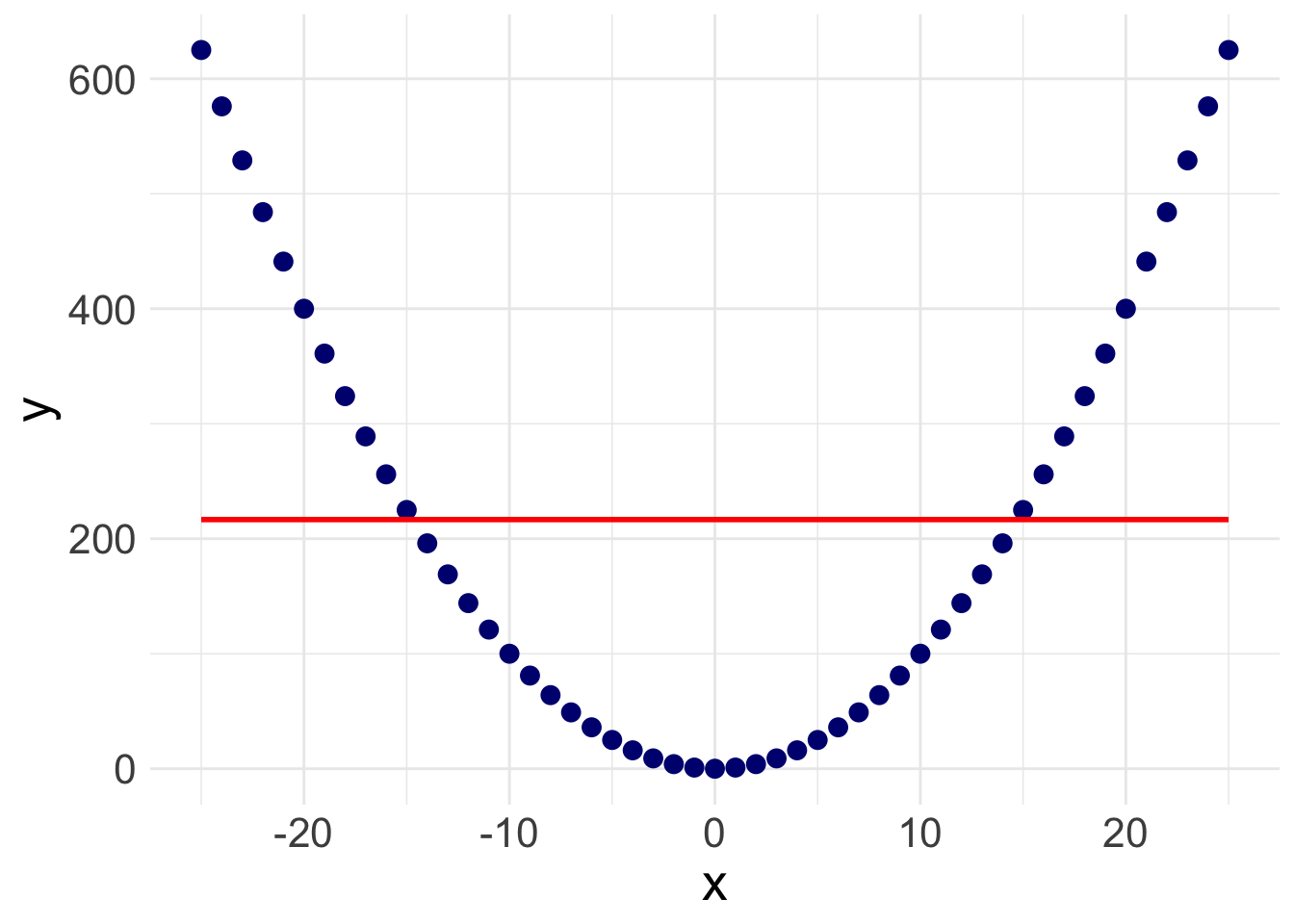
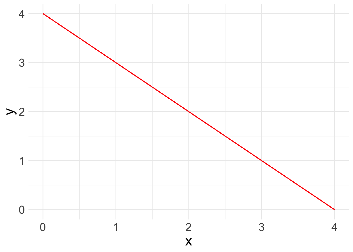
There is a slight slope to the line, indicating we may have a significant linear relationship. However, Stata will plot a straight line even if the relationship is NOT linear. Take the following example. Here, I’ve plotted a data set with a parabolic relationship ( \(y = x^2\) ) and then plotted a line of best fit. Even though there is a clear relationship, it’s a curved relationship, not a linear one. Our line of best fit is misleading.

So how do we overcome this problem? Rather than assuming a linear relationship, we can instead plot a ‘lowess’ curve onto our graph.

Lowess Curve

A Lowess (Locally Weighted Scatterplot Smoothing) curve creates a smooth line showing the relationship between your independent and dependent variables. It is sometimes called a Loess curve (there is no difference). Basically, the procedure cuts your data into a bunch of tiny chunks and runs a linear regression on those small pieces. It is weighted in the sense that it accounts for outliers, showing possible curves in the relationship between your two variables. Lowess then combines all the mini regression lines into a smooth line through the scatter plot. Here is a long, mathematical explanation for those of you who are interested. All you need to know is that it plots a line that may or may not be linear, letting you see at a glance if there is a big problem in your linearity assumption.

Again, all you have to do is add the lowess command to the end of your scatterplot.

scatter wealthworthinbillions age || lowess wealthworthinbillions age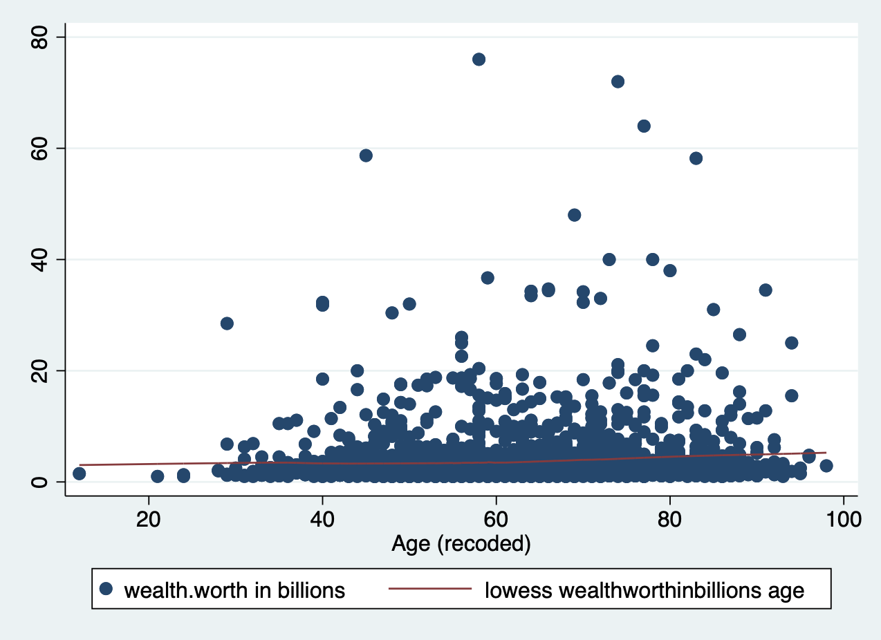

Does this result count as a ‘linear’ relationship?

Research Note

Evaluating linearity, as with many aspects of quantitative research, involves subjective interpretation. Sometimes the nonlinearity will jump out at you, and sometimes it won’t. You have to think carefully about what does or doesn’t count as linear. This is just one method.

Correlation

Another way to evaluate for a linear relationship is looking at the correlation between your variables. You may or may not remember correlation from your introductory statistics classes. A quick review…

Correlation refers to the extent to which two variables change together. Does x increase as y increases? Does y decrease as x decreases? If whether or not one variable changes is in no way related to how the other variable changes, there is no correlation. In mathematical terms, the correlation coefficient (the number you are about to calculate) is the covariance divided by the product of the standard deviations. Again, here’s a mathematical explanation if you are interested. What you need to know is that the correlation coefficient can tell you how strong the relationship between two variables is and what direction the relationship is in, positive or negative. Of course, we must always remember that correlation \(\neq\) causation.

There are actually a number of different ways to calculate a correlation (aka. a correlation coefficient) in Stata.

Option 1:

correlate wealthworthinbillions age female2

(obs=2,229)

             | wealth~s      age  female2
-------------+---------------------------
wealthwort~s |   1.0000
         age |   0.0859   1.0000
     female2 |   0.0220  -0.0152   1.0000

Option one correlate (very intuitive command) uses “listwise deletion” to deal with missing values. If an observation is missing on ANY of the variables you are correlating it automatically deletes them from the entire correlation matrix.

Option 2:

pwcorr wealthworthinbillions age female2, sig    

             | wealth~s      age  female2
-------------+---------------------------
wealthwort~s |   1.0000 
             |
             |
         age |   0.0859   1.0000 
             |   0.0000
             |
     female2 |   0.0175  -0.0152   1.0000 
             |   0.3754   0.4719
             |

The command pwcorr does a number of things differently. First, it uses “pairwise deletion,” meaning it excludes an observation from the correlation calculation of each pair of correlations (i.e., if there are missing values on age, but not the other variables). Second, it allows you to see whether the correlations are statistically significant. The option sig above places the p-values on in your correlation table. The option star (0.05) below sets the alpha to p = 0.05 and places a star next to the statistically significant values. You can see that the correlation between age and wealth is the only significant correlation.

pwcorr wealthworthinbillions age female2, star (0.05)

             | wealth~s      age  female2
-------------+---------------------------
wealthwort~s |   1.0000 
         age |   0.0859*  1.0000 
     female2 |   0.0175  -0.0152   1.0000 

Now we know that there is a significant, positive correlation between wealth and age. It’s time to run a linear regression.

Research Note

In the future, it is going to be important for you to know whether or not your independent variables are correlated with one another. This is called collinearity, and it can cause all sorts of problems for your analysis. Keep these correlation commands in your toolbelt for the future.

4.4 Running a Basic Linear Regression

Refresh: What is a linear regression model anyways?

Now you are ready to run a basic linear regression! With a linear regression, you are looking for a relationship between two or more variables: one or more x’s and a y. Because we are looking at linear relationships, we are assuming a relatively simple association. We may find that either as x increases, y increases: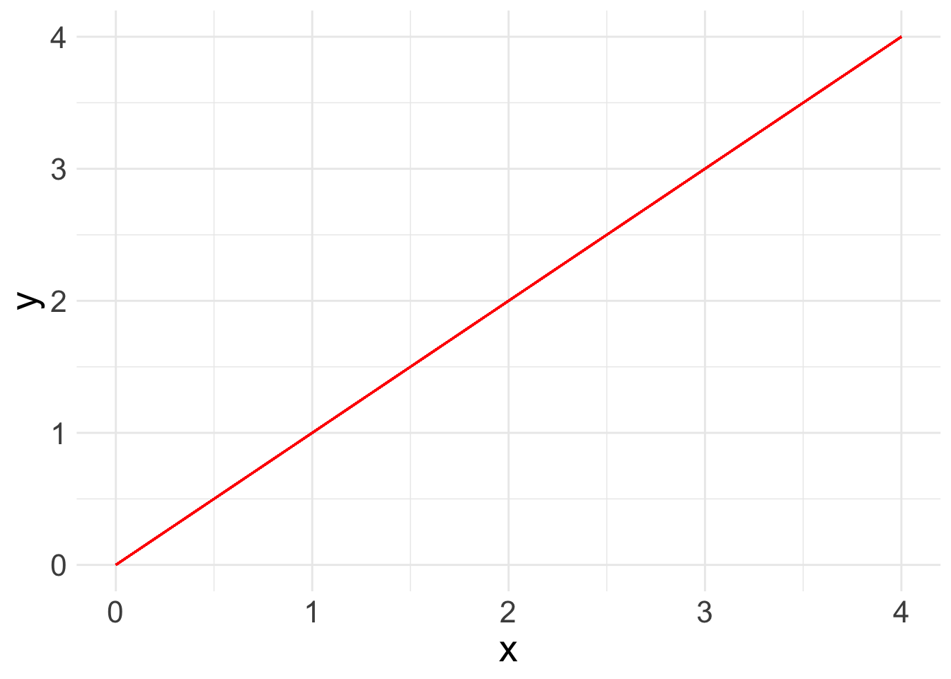
We may find that as x increases, y decreases:

What a linear regression analysis tells us is the slope of that relationship. The slope is what we want to learn from linear regression. This is the linear formula you may be used to seeing:
\[ y = ax + b\]
Because statisticians love to throw different annotation at us, here’s the same equation as you will see it in linear regression books:
\[ y_i = A + \beta x_i\]
In this equation:

• \(y_i\): refers the value of the outcome for any observation
• \(A\): refers to the intercept or constant for your linear regression line
  
• \(x_i\): refers to the value of the independent variable for any observation
• \(\beta\): refers to the slope or “coefficient” of the line.

When we add more variables of interest, or “covariates”, we also add them in as X’s with a subscript. The betas ( \(\beta\) ) also take on a subscript. So a linear equation with three covariates would look like:
\[ y_i = A + \beta_1 x_{1i} + \beta_2 x_{2i} + \beta_3 x_{3i}\] In general terms, this equation means that for any observation if I want to know the value of y, I have to add the constant (\(A\)) plus the value for \(x_1\) times its coefficient, plus the value for \(x_2\) times its coefficient, plus the value for \(x_3\) times its coefficient.

However, the line that linear regression spits out isn’t perfect. There’s going to be some distance between the value that is predicted and what the actual value is according to our equation. This is called the “error” or the “residual” The whole point of linear regression estimation is to minimize the error. We refer to the error with the term \(e_i\). Each observation has its own error term or residual, aka the amount that the true value of that observation is off from what our regression line predicts. We’ll play more with residuals in the next lab.

So the final equation in a linear regression is:
\[ y_i = A + \beta_1 x_{1i} + \beta_2 x_{2i} + \beta_3 x_{3i} + e_i\]

Run your model in Stata with regress

Now let’s look at a real example with data: what is the relationship between a billionaire’s wealth and their gender and age. The equation for this regression would be:
\[ y_{wealth} = A + \beta_1 x_{gender} + \beta_2 x_{age} + e_i\]

regress wealthworthinbillions female age 

The code is simple enough. You are actually writing out the formula above, just without the equals sign. Always put your outcome variable ( y ) first followed by any independent variables ( x ). The logic is that you are regressing \(y\) (wealth), on \(x_1\) (gender) and \(x_2\) (age).

Interpreting the output

I have broken down understanding the output into two parts. First, what are the findings of the model? Second, is this a good model or not?

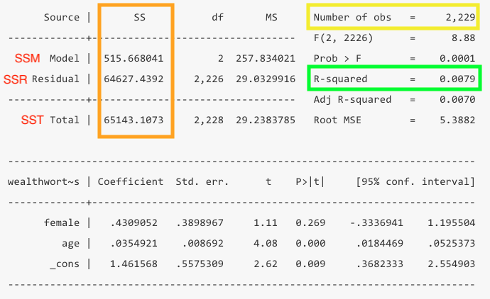
What are the findings?

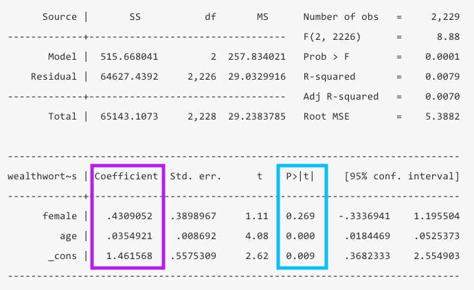
When you glance at a regression table, you want to know at a glance what the findings are and if they are significant. The two main columns you want to look at are the values for the Coefficients in purple and the p-values (P>|t|) in blue.

• The coefficients are your \(\beta\) values. We can interpret these by saying “For every one unit increase in x, y increases by \(\beta\).” In this example, for every year that age increases, wealth increases by .034 billion dollars.
• The _const value in the coefficient column is your intercept or constant. The A in your equation above. In this case it means when both female and age are zero, wealth is 1.46 billion. Of course age being zero doesn’t make much sense, so in this model it is not very informative to interpret the constant.
  
• The p-values tell you whether your coefficients are significantly different from zero. In this example, the coefficient for age is significant, but the coefficient for gender is not.
• You can also look at the 95% confidence interval to see if it contains 0 for significance, but it will align with the p-value. If your confidence interval is super wide, that can be an indicator that your results aren’t precise or your sample size is too small.

4.4.0.1 How good is this model?

Now that you know your findings, you still need to take a step back and evaluate how good this model is. To do so, you’ll want to look at the the total number of observations in yellow, the R-squared in green, which is calculated from the sum of squares values in orange.

• Number of observations: You should take note of the number of observations to ensure it is not wildly different than what you expected. If you have a significant amount of missing values in your dataset, you may lose a bunch of observations in your model.
• R-squared: This value tells us at a glance how much explanatory power this model has. It can be interpreted as the share of the variation in y that is explained by this model. In this example only 0.79% of the variation is explained by the model.
• The R-squared is a function of the sum of squares. The “sum of squares” refers to the variation around the mean.
  • SSTotal = The total variation around the mean squared (\(\sum{(Y - \bar{Y}})^2\))
  • SSResidual = The sum of squared errors (\(\sum{(Y - Y_{predicted}})^2\))
  • SSModel = How much variance the model predicts (\(\sum{(Y_{predicted} - \bar{Y}})^2\))
  • The SSTotal = SSModel + SSResidual and the R-squared = SSModel/SSTotal. Note: You don’t need to calculate this, Stata does it for you, but it’s good to know what the logic is.

Here’s a useful webpage explaining each piece of the regression output in Stata if you want more information.

Important variations in the regress command

Categorical independent variables

Stata has a specific way of handling categorical variables in a regression. In our first example, we actually put in gender as a continuous variable. By default, Stata assumes each variable is continuous. To tell Stata a variable is categorical you have to put a i. in front of the variable name. The i. stands for indicator variable. Another way of saying categorical. If you wanted to be exact, you could add c. in front of a variable to specify that it is continuous. Although it is not strictly necessary, since Stata will assume it is continuous.

Let’s rerun our example above, correctly specifying our variable female as a categorical variable. Notice how our female variable now shows the name of the variable, and beneath it the actual value labeled one.

regress wealthworthinbillions i.female c.age

      Source |       SS           df       MS      Number of obs   =     2,229
-------------+----------------------------------   F(2, 2226)      =      8.88
       Model |  515.668041         2  257.834021   Prob > F        =    0.0001
    Residual |  64627.4392     2,226  29.0329916   R-squared       =    0.0079
-------------+----------------------------------   Adj R-squared   =    0.0070
       Total |  65143.1073     2,228  29.2383785   Root MSE        =    5.3882

------------------------------------------------------------------------------
wealthwort~s | Coefficient  Std. err.      t    P>|t|     [95% conf. interval]
-------------+----------------------------------------------------------------
      female |
     Female  |   .4309052   .3898967     1.11   0.269    -.3336941    1.195504
         age |   .0354921    .008692     4.08   0.000     .0184469    .0525373
       _cons |   1.461568   .5575309     2.62   0.009     .3682333    2.554903
------------------------------------------------------------------------------

Stata’s automatic response is to treat any variable as “a ONE unit difference in.” While that makes sense for continuous and MOST ordinal variables, that doesn’t really make sense for nominal variables, especially those with more than two categories. It doesn’t make much difference here though, but in the future it will. Using this notation is useful to make sure you (and Stata) are always aware what each variable is.

Running regressions on subsets

Sometimes, you want to run a regression on a subsample of people in your dataset. The if command lets you specify what that subgroup is (I selected observations with billionaires whose wealth was inherited).

regress wealthworthinbillions i.female c.age if wealthtype2 == 3

      Source |       SS           df       MS      Number of obs   =       765
-------------+----------------------------------   F(2, 762)       =      7.99
       Model |  372.207956         2  186.103978   Prob > F        =    0.0004
    Residual |  17754.1282       762  23.2993809   R-squared       =    0.0205
-------------+----------------------------------   Adj R-squared   =    0.0180
       Total |  18126.3362       764  23.7255709   Root MSE        =    4.8269

------------------------------------------------------------------------------
wealthwort~s | Coefficient  Std. err.      t    P>|t|     [95% conf. interval]
-------------+----------------------------------------------------------------
      female |
     Female  |   .5844082   .4130495     1.41   0.158    -.2264418    1.395258
         age |   .0482612   .0128561     3.75   0.000     .0230236    .0734988
       _cons |   .8206522    .830654     0.99   0.323    -.8099897    2.451294
------------------------------------------------------------------------------

Notice how the number of observations changes.

4.5 Challenge Activity

1. Run another regression with wealth as your outcome and two new variables. Note: You may need to clean these variables before you use them.
   

2. Interpret your output in plain language (aka. “A one unit change in x results in…”) and whether it is statistically significant.

This activity is not in any way graded, but if you’d like me to give you feedback email me your .do file and a few sentences interpreting your results.