10 Day 9
Review
Sample Mean
\[\bar{x} = {1 \over n}\sum\limits_{i=1}^nx_i\]
\[\bar{y} = {1 \over n}\sum\limits_{i=1}^ny_i\]
Sample Variance
\[s_x^2 = {{{\sum\limits_{i=1}^n}(x_i-\bar{x})^2}\over (n-1)}\]
\[s_y^2 = {{{\sum\limits_{i=1}^n}(y_i-\bar{y})^2}\over (n-1)}\]
Sample Standard Deviation
\[\sqrt{s_x^2}=s_x\]
\[\sqrt{s_y^2}=s_y\]
Correlation Coefficient
Given \(n\) ordered pairs (\(x_i,y_i\))
With sample means \(\bar{x}\) and \(\bar{y}\)
Sample standard deviations \(s_x\) and \(s_y\)
The correlation coefficient \(r\) is given by:
\[r = \frac{1}{n-1} \sum_i \left( \frac{x_i - \bar{x}}{s_x} \right) \left( \frac{y_i - \bar{y}}{s_y} \right)\]
Correlation Coefficient Properties:
- The value is always between \(-1 \le r \le 1\)
If \(r=1\), all of the data falls on a line with a positive slope
If \(r=-1\) all of the data falls on a line with a negative slope
The closer \(r\) is to 0, the weaker the linear relationship between \(x\) and \(y\)
If \(r=0\) no linear relationship exists
- The correlation does not depend on the unit of measurement for the two variables
- Correlation is very sensitive to outliers
- Correlation measures only the linear relationship and may not (by itself) detect a nonlinear relationship
Housing Example:
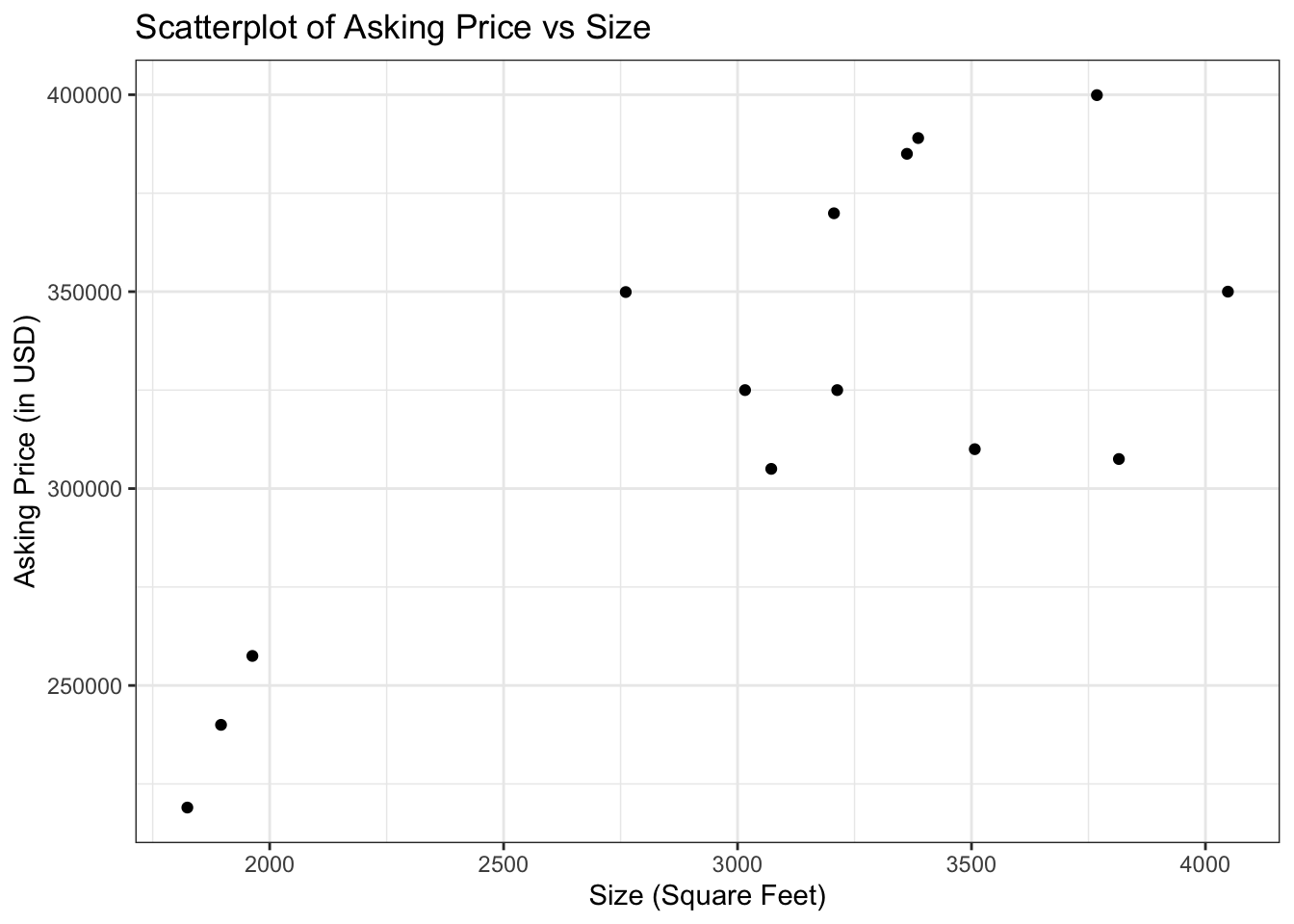
We can draw a line through this data:
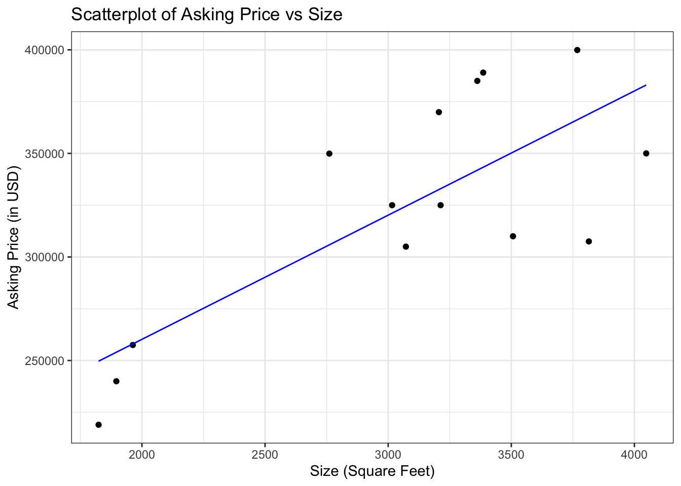
We come up with this line using Least Squares Regression:
Given ordered pairs (\(x,y\))
With sample means \(\bar{x}\) and \(\bar{y}\)
Sample standard deviations \(s_x\) and \(s_y\)
Correlation coefficient \(r\)
The equation of the least-squares regression line for predicting \(y\) from \(x\) is:
\[\hat{y}=\beta_0+\beta_1x\]
Where the slope (\(\beta_1\)) is:
\[\beta_1 = r * {s_y\over s_x}\]
And the intercept (\(\beta_0\)) is:
\[\beta_0=\bar{y}-\beta_1 \bar{x}\]
What do we call \(y\)?
\(x\)?
\(\beta_0\)?
\(\beta_1\)?
\(\hat{y}\)?
How do we interpret \(\beta_0\) and \(\beta_1\)?
Probability
Why do we study probability in statistics?
Let’s propose a research question:
How much do K-State students spend on average on books and supplies every semester?
What’s my population?
What measurement am I making inference on?
How can I sample for this population?
What will I calculate from my sample?
Is what I calculate exact to reality?
Probability
- A number between \(0\) and \(1\) that tells us how likely a given “event” is to occur
Probability equal to \(0\) means the event cannot occur
- \(P(x)=0\)
Probability equal to \(1\) means the event must occur
- \(P(x)=1\)
Probability equal to \(1/2\) means the event is as likely to occur as it is to not occur
- \(P(x)=0.5\)
Probability close to 0 (but not equal to 0) means the event is very unlikely to occur
The event may still occur, but we’d tend to be surprised if it did
\(x=\{\text{A shark attack on a beach in the U.S.}\}\)
\(P(x) \approx 0.00000008\)
But \(P(x) \ne 0\)
Probability close to 1 (but not equal to 1) means the event is very likely to occur
The event may not occur, but we’d tend to be surprised if it didn’t
\(x=\{ \text{You lose the national lottery you bought a ticket for} \}\)
\(P(x) \approx 0.999999997\)
\(P(x) \ne 1\)
- Do not gamble
Probability Terminology
To study probability formally, we need some basic terminology
Experiment (in context of probability):
- An activity that results in a definite outcome where the observed outcome is determined by chance
Sample space:
- The set of ALL possible outcomes of an experiment; denoted by \(S\)
- Flip a coin once
\[S = \{H, T\}\]
- Randomly select a person and then determine blood type
\[S = \{A, B, AB, O\}\]
Event
A subset of outcomes belonging to sample space \(S\)
A capital letter towards the beginning of the alphabet is used to denote an event
- i.e. \(A\), \(B\), \(C\), etc.
- Suppose we flip a coin twice
\[S = \{HH, HT, TH, TT\}\]
- Let \(A\) be the event we observe at least one tails
\[A = \{HT, TH, TT\}\]
- Let \(B\) be the event we observe at most one tails
\[B = \{HH, HT, TH\}\]
Simple event
- An event containing a single outcome in the sample space \(S\)
- Example:
\[S = \{HH, HT, TH, TT\}\]
Let \(A = "\)we observe two heads\("\) \(= \{HH\}\) is a simple event
Compound event
- An event formed by combining two or more events (thereby containing two or more outcomes in the sample space \(S\))
- Example:
\[S = \{HH, HT, TH, TT\}\]
Let \(B = "\)we observe a head in the first or in the second flip\("\) \(= \{HT, TH, HH\}\) is a compound event
Probability Methods
There are 3 general views of probability
Consider these as methods of assigning probabilities to events
Subjective Probability
Probability is assigned based on judgement or experience
i.e. expert opinion, personal experience, “vibe math”
Examples:
A doctor assessing the chance of a patient recovering from a medical procedure
A managerial team estimating the probability a project will achieve technical success
This probability may not be expressed in an actual number; instead, we may say “low”, “high”, “almost certain”, etc.
Classical Probability
Make some assumptions in order to build a mathematical model from which we can derive probabilities
- It’s not vibe math but it can definitely feel like it
Example: Suppose we want to put a probability on the event of observing “tails” in one flip of a coin. We might assume the following:
there are only 2 possible outcomes: “heads” or “tails”
the coin is “fair”, i.e. heads & tails have an equal chance of occurring
Therefore, based on our model,
\[\text{the probability of observing tails} = P(\text{tails}) = \frac{1}{2}.\]
Note: This is an example of an equally-likely probability model (i.e., all possible outcomes are equally likely to occur) where
\[P(A) = \frac{\text{number of outcomes in event } A}{\text{total number of outcomes in } S}.\]
- Here \(P(A)\) denotes the probability of the event \(A\)
Relative or Empirical Probability
- Think of the probability of an event as the proportion of times that the event occurs
Example: For our flip of a tack:
\[P(\text{point up}) = \text{the proportion of all possible flips of the tack where it lands “point up”}\]
Under the relative frequency view of probability, we can estimate the probability of an event from a sample
We could flip our tack a large number of times, say \(1000\), and count the number of times it lands point up
This is like a simple random sample (SRS) from the population of all tack flips
\[P(\text{point up}) \approx \frac{\text{number of times “point up” is observed}}{1000}\]
Law of Large Numbers
As the size of our sample (i.e., number of experiments) gets larger and larger:
The relative frequency of the event of our interest gets closer and closer to the true probability
What does this mean to us?
You can get as close as needed to the true probability by taking a large enough sample
It is also used to justify the relative frequency view of probability
This is how some statisticians evaluate new statistical procedures; they simulate many datasets and observe the proportion of time the procedure “works”
Example 1: Classical Probability
Assume that a fair die is rolled (i.e., all outcomes are equally-likely).
- Write down the sample space.
- Find the probability of rolling a 5.
- Find the probability of rolling an even number.
- Find the probability of rolling a number less than 3.
Example 2: Empirical Probability
An automobile insurance company divides customers into three categories: good risks, medium risks, and poor risks. Assume that of a total of \(11,217\) customers, \(7792\) are good risks, \(2478\) are medium risks, and \(947\) are poor risks. As part of an audit, one customer is chosen at random.
For each probability, give the exact answer or round to four decimal places.
- What is the probability that the customer is a good risk?
- What is the probability that the customer is not a poor risk?
Live Example: Empirical Probability
Say you flip a coin twice:
- What is the sample space?
- What is the probability, given the sample space, of having at least one heads?
- What is the probability of at least one heads if you flip a coin three times?
- Can you reasonably prove it?
- Let’s actually flip a coin “a few times”