9 Day 8
Review
- Recall the 5 Number Summary:
| Metric | Min | Q1 | Median | Q3 | Max |
| Value | 53 | 70 | 78 | 82 | 91 |
- And how we can convert this to a boxplot:
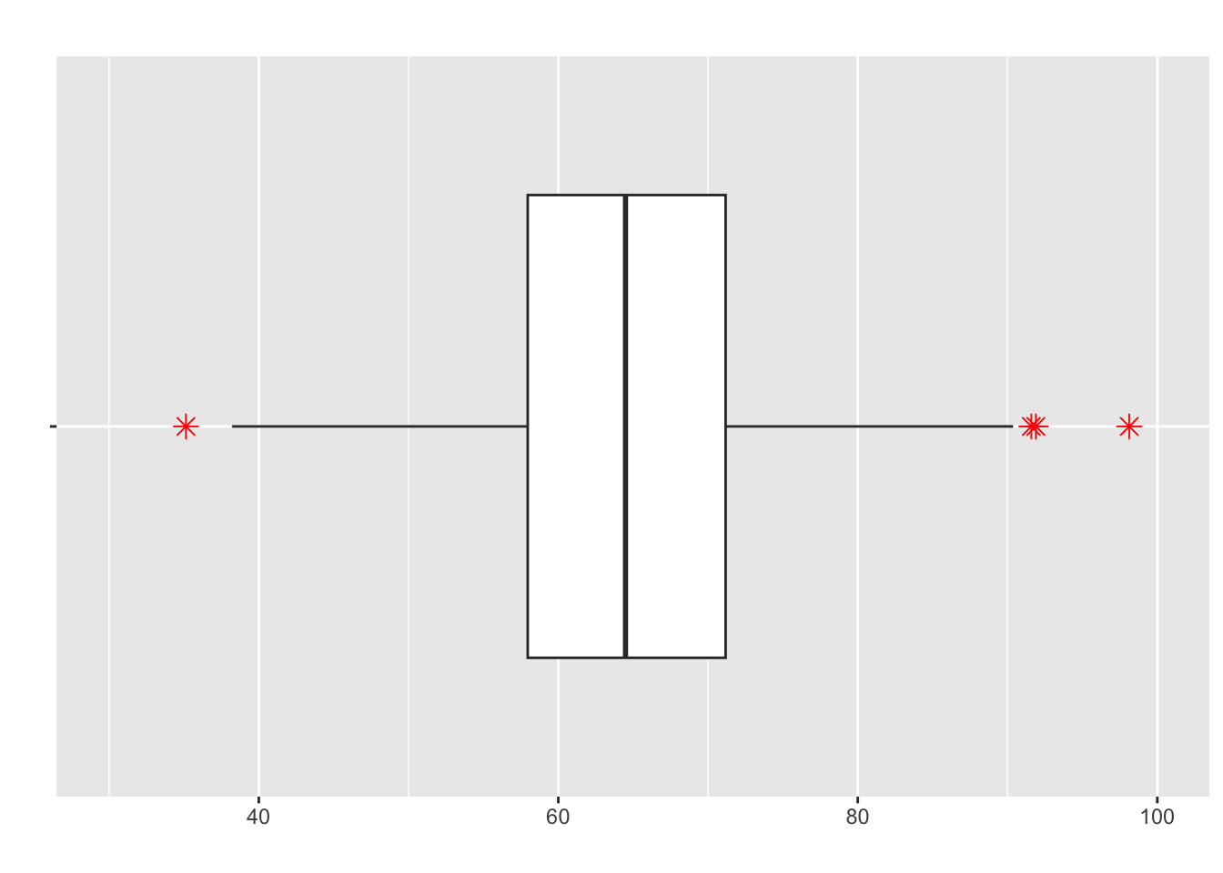
What are the componenets of the 5 number summary on this boxplot?
What are the stars?
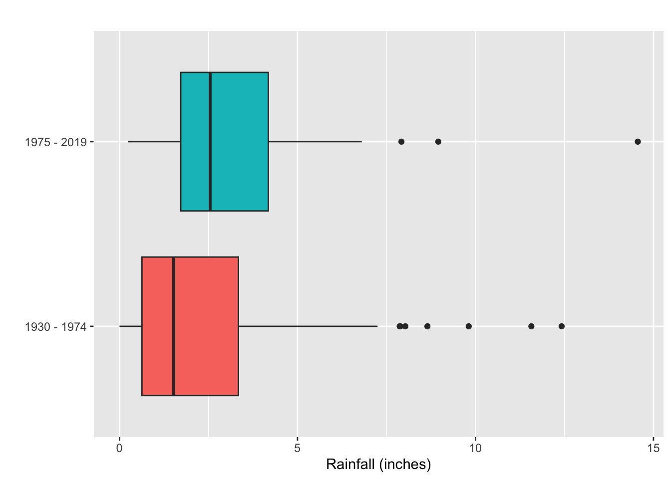
- Boxplots are best used for comparing two data sets:
When we have two quantitative variables we use scatterplots
Define one variable as \(x\) and one as \(y\)
Given \(x_i\) is the \(i^{th}\) data point in the \(x\) set
\(y_i\) is the \(i^{th}\) data point in the \(y\) set
- The data set should be:
\[(x_1,y_1),(x_2,y_2),...,(x_n,y_n)\]
- What is this called?
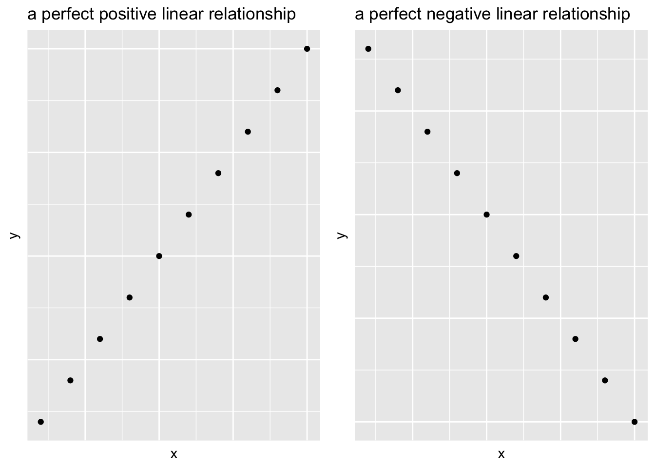
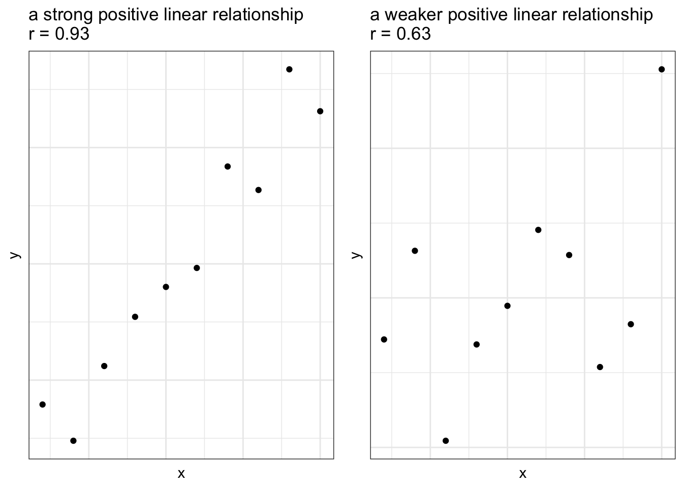
For any two variables we can define their relationship as a:
Positive association if large values of one variable are associated with large values of another
Negative association if large values of one variable are associated with small values of another
Two variables can have a linear relationship if the data tend to cluster around a straight line when plotted on a scatterplot
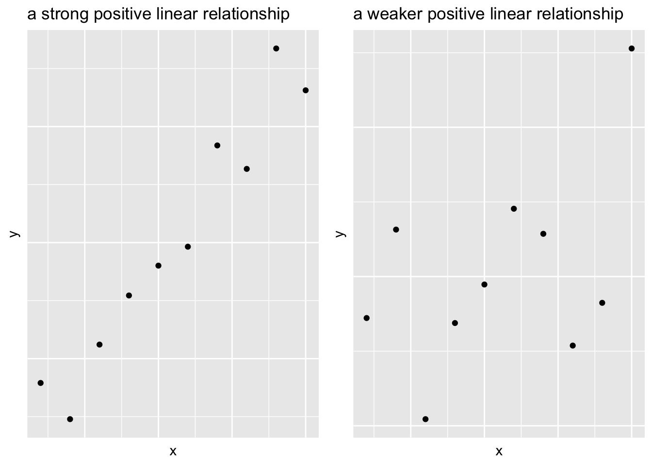
Strength of Linear Relationship
When two variables have a linear relationship
- It’s useful to quantify how strong the relationship is
Visual impressions aren’t really reliable
- Axis scaling can change everything:
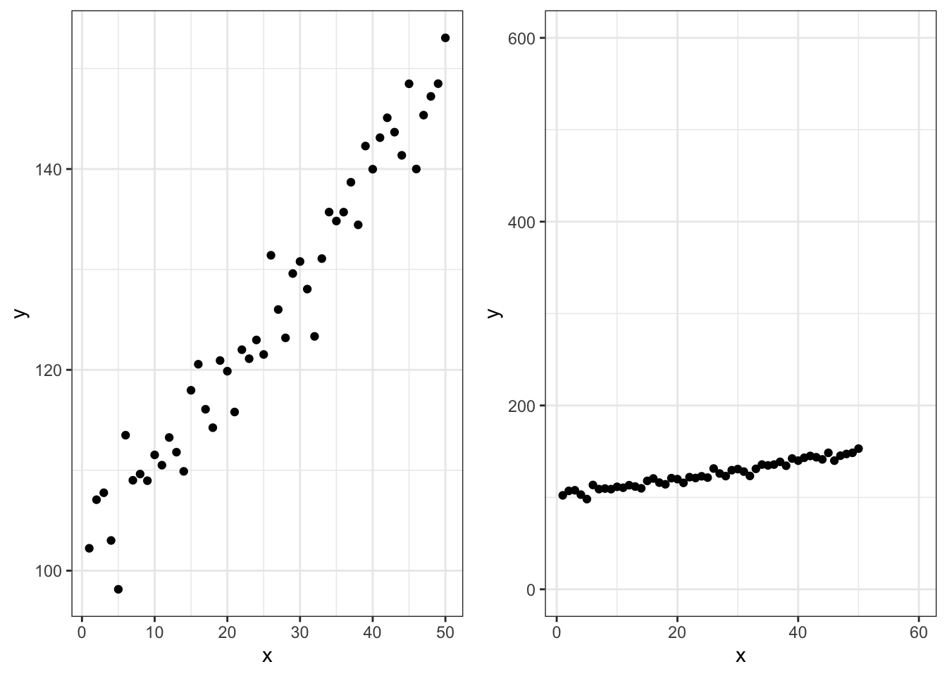
- This is the same data, plotting in two different ways
Correlation Coefficient
Numerical measurement of the strength (and direction) of the linear relationship between two quantitative variables.
Given \(n\) ordered pairs (\(x_i,y_i\))
With sample means \(\bar{x}\) and \(\bar{y}\)
Sample standard deviations \(s_x\) and \(s_y\)
The correlation coefficient \(r\) is given by:
\[r = \frac{1}{n-1} \sum_i \left( \frac{x_i - \bar{x}}{s_x} \right) \left( \frac{y_i - \bar{y}}{s_y} \right)\]
Does anything look familiar here?
Properties of the Correlation Coefficient
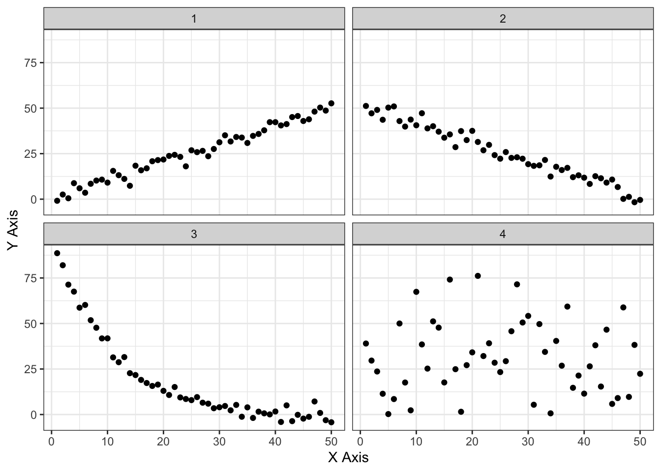
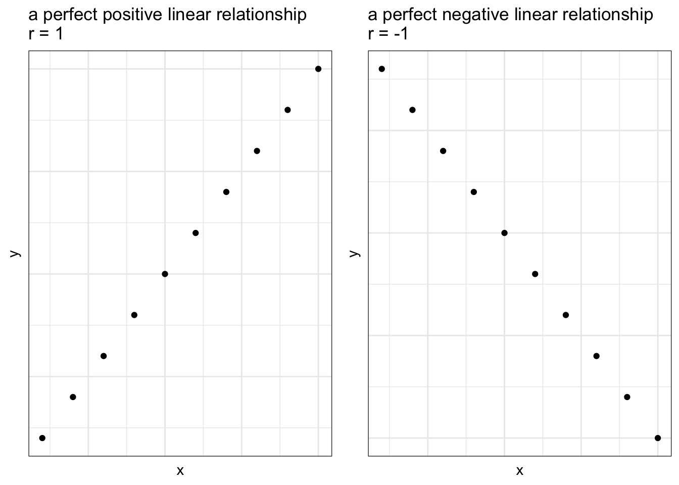
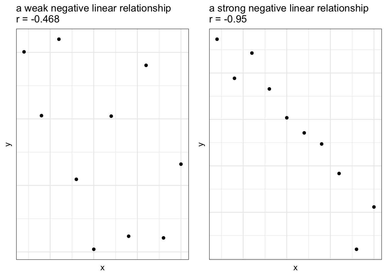
- The value is always between \(-1 \le r \le 1\)
If \(r=1\), all of the data falls on a line with a positive slope
If \(r=-1\) all of the data falls on a line with a negative slope
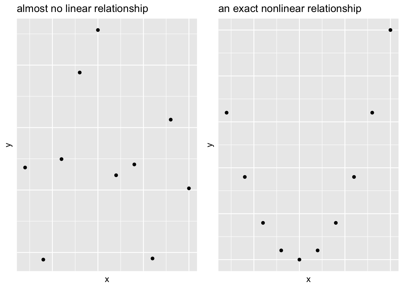
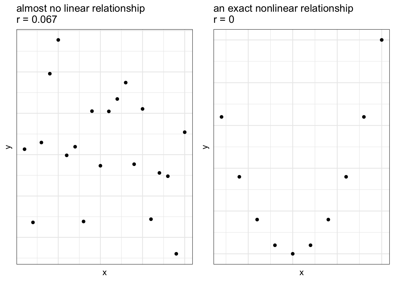
The closer \(r\) is to 0, the weaker the linear relationship between \(x\) and \(y\)
If \(r=0\) no linear relationship exists
- The correlation does not depend on the unit of measurement for the two variables
- \(x\) is House price and \(y\) is \(ft^2\), but they can still have \(r\) calculated
- Correlation is very sensitive to outliers.
One point that does not belong in the dataset can result in a misleading correlation
Always plot your data!
Would we say this measurement is resistant or not?
- Correlation measures only the linear relationship and may not (by itself) detect a nonlinear relationship
Example 2: Least Squares Regression Line
- Recall the MHK House example:
| Square Feet | Asking Price (in USD) |
|---|---|
| 2761 | 349900 |
| 1824 | 219000 |
| 3362 | 385000 |
| 4048 | 350000 |
| 3016 | 325000 |
| 3768 | 399900 |
| 3072 | 305000 |
| 3815 | 307500 |
| 3213 | 325000 |
| 1963 | 257500 |
| 3507 | 310000 |
| 3386 | 389000 |
| 1896 | 240000 |
| 3206 | 369900 |
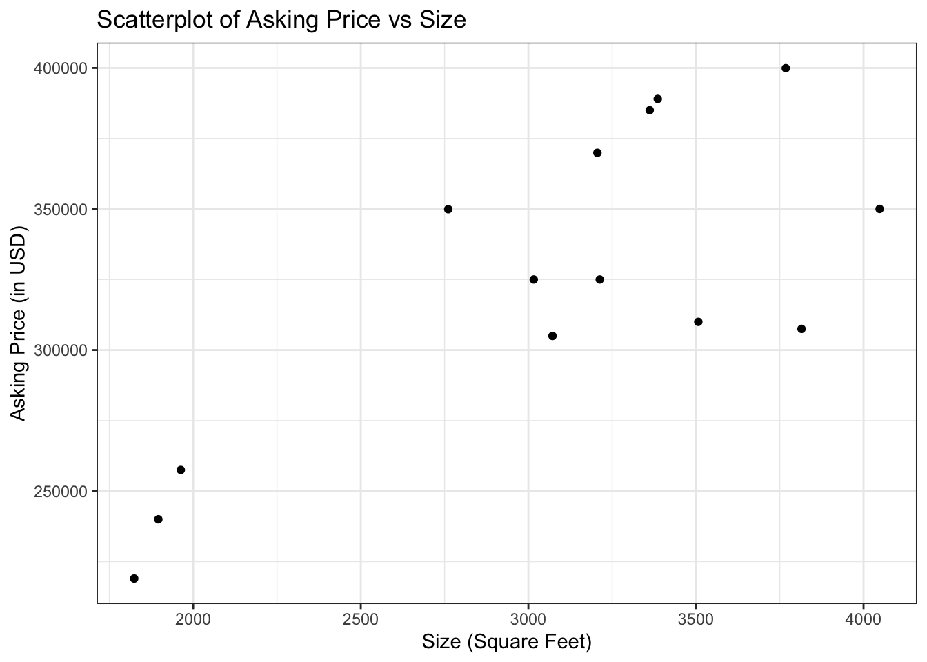
Each home has a value for its asking price (in dollars) and another for the size of its living space (in square feet)
- Two variables for each individual in the sample
\(x=\) size of the living space
\(y=\) asking price of the home
For the \(i^{th}\) home, we’ll denote it’s observated values as:
\(x_i=\) the size of the \(i^{th}\) home in \(ft^2\)
\(y_i=\) the asking price of the \(i^{th}\) home in dollars
The associated scatterplot:
- As I’ve said before, we can draw a line through this plot:
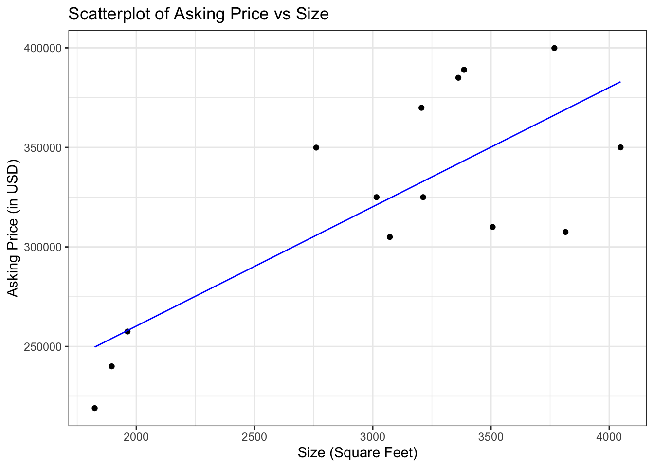
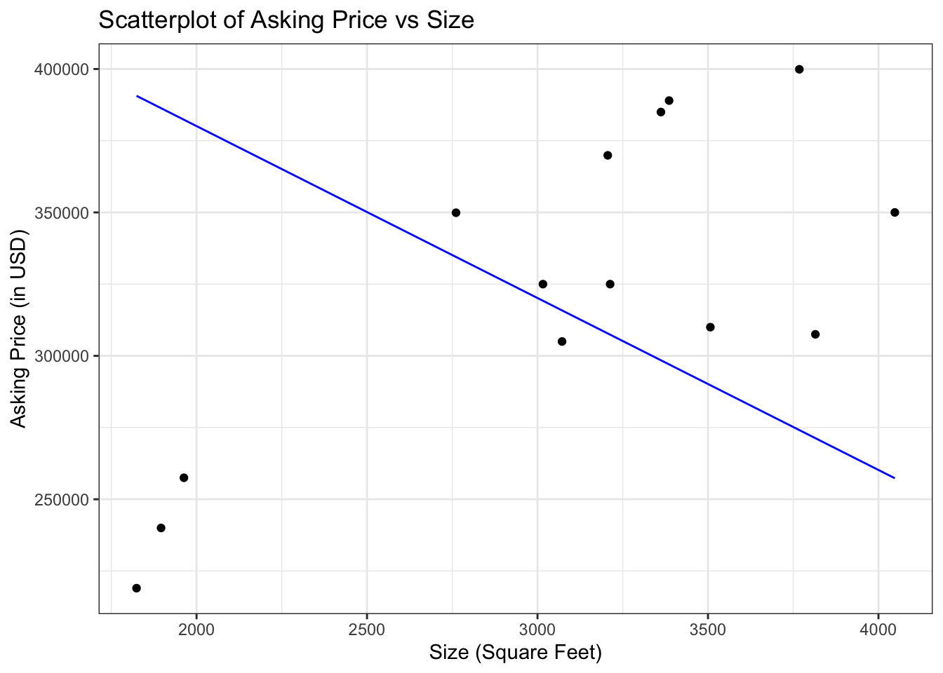
Above scatter plots presents each with a different line superimposed
- We can see intuitively which is the better line, but there’s a deeper reason
The reason being the vertical distances are on whole smaller for the first line
We determine exactly how well the line fits by squaring the vertical distances and adding them up
The line that fits best is the line for which the sum of squared distances is as small as possible
This line is known as the Least Squared Regression Line
Least-Squares Regression
Given ordered pairs (\(x,y\))
With sample means \(\bar{x}\) and \(\bar{y}\)
Sample standard deviations \(s_x\) and \(s_y\)
Correlation coefficient \(r\)
The equation of the least-squares regression line for predicting \(y\) from \(x\) is:
\[\hat{y}=\beta_0+\beta_1x\]
Where the slope (\(\beta_1\)) is:
\[\beta_1 = r * {s_y\over s_x}\]
And the intercept (\(\beta_0\)) is:
\[\beta_0=\bar{y}-\beta_1 \bar{x}\]
In general:
The variable we want to predict is the outcome or response variable
And the variable we are given is the explanatory or predictor variable
Example 3: Applying Least Squares Regression
Using the data from Example 2 find the least-squares regression line for predicting the price from the size given:
\[\bar{x}= 2891.25,\ \bar{y}=447.0 ,\ s_x=269.49357 ,\ s_y= 29.68405,\ r=0.9005918\]
\[\beta_1 = r * {s_y\over s_x}\]
\[\beta_0=\bar{y}-\beta_1 \bar{x}\]
\[\hat{y}=\beta_0+\beta_1x\]
Given our regression equation, predict the value of a house at 2800 square feet
Interpretation of Least Squares Regression
Interpreting the predicted \(\hat{y}\)
The predicted value of \(\hat{y}\) can be used to estimate the average outcome for a given value of the explanatory variable \(x\)
For any given value of \(x\), the value \(\hat{y}\) is an estimate of the average \(y\)-value for all points with that \(x\)-value
From above example we estimate that average price of house of size \(2800\) square feet to be \(\$ 438,000\)
Interpreting \(y\)-intercept \(b_0\)
The y-intercept is \(b_0\) is the point where the line crosses \(y\)-axis. This has two meanings
If the data has both positive and negative \(x\)-values the \(y\)-intercept is the estimated outcome when the value of explanatory variable is \(0\)
If the x-values are all positive or all negative then \(b_0\) does not have useful information.
Interpreting the slope \(b_1\)
- If the x-values of two points differ by 1, their \(y\)-values will differ by an amount equal to the slope of the line
LSR Examples
Example 1:
- Two houses are up for sale and one is \(1900\) square feet and the other is \(1750\) square feet. By how much should we predict their houses to differ?
- The difference in size is \(150\). The slope of the least-square line is \(b_1 = 0.0992\). We predict the prices to differ by \(150 \times 0.0992 = 14.9\) thousand dollars, or \(\$ 14,900\).
Example 2 (pg. 184):
At the final exam the professor asked each student to indicate how many hours they have studied for the exam.
The professor computes the least-square regression line for predicting the final exam scores from the number of hours studied.
-The equation of the line is \(\hat{y} = 50 + 5x\).
- Antoine has studied for \(6\) hours. What do you predict his score would be?
- Emma studied \(3\) hours more than Jeremy did. How much higher do you predict Emma’s score to be?
Example 3:
- Is there an interpretation of the \(y\)-intercept?
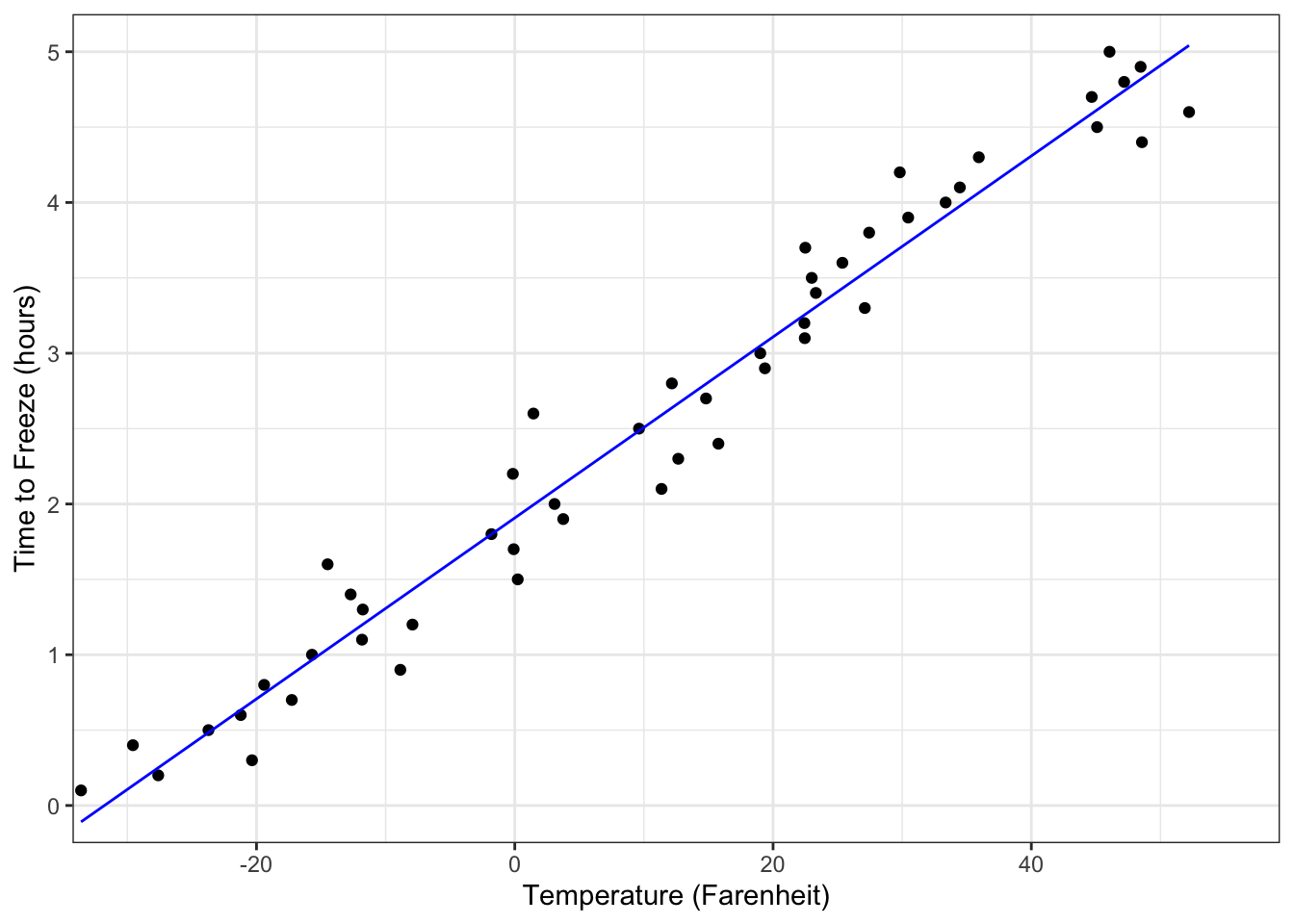
The least square regression line is \(\hat{y} = 1.908 + 0.06x\) where \(x\) is temperature in freezer in Fahrenheit and \(y\) is the time it takes to freeze.
Example 4:
- Is there an interpretation of the \(y\)-intercept?
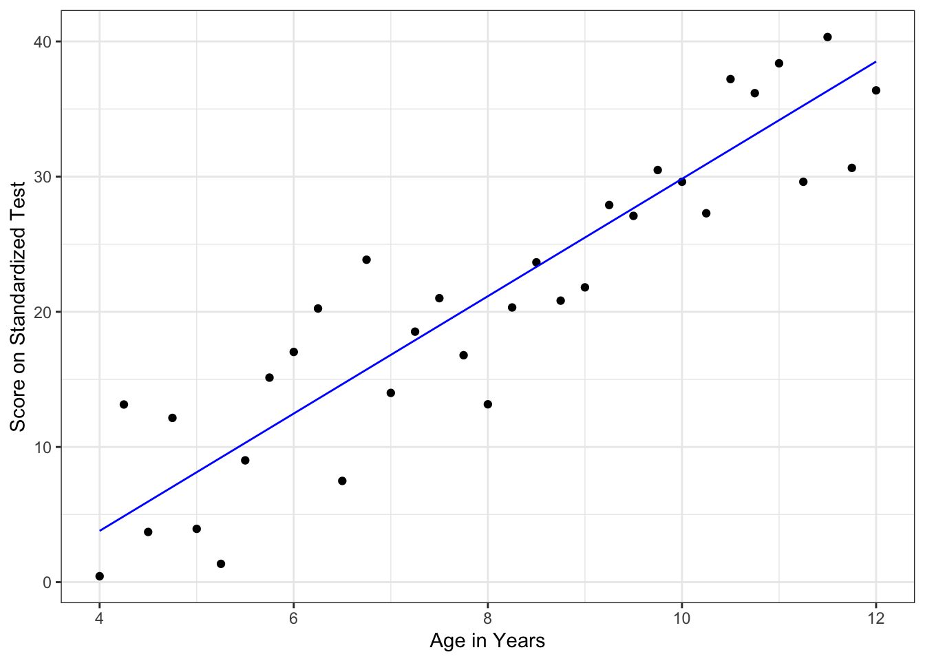
The least square regression line is \(\hat{y} = -13.568 + 4.340x\) where \(x\) is the age of an elementary school student and \(y\) is the score on the standard test.
- Go away