13 Day 12
Announcements
Midterms looked good
Scores haven’t been posted yet
That is entirely out of my control
I will not expedite that process because I am physically incapable of doing that
THIS WAS THE EASY EXAM
If you found the exam trivial, don’t resolve to stop attending class
The next exam will ruin you if you don’t come to class and learn the content
Think of class time as a version of study time
The probability that your study time is more efficient than class time is low
Source: I’ve been doing this (being a student) longer than you
If you found the exam difficult/brutal, start attending office hours and help lab
The content we cover from here on out is not nearly as intuitive
Some would argue portions of it are counter-intuitive
- \(\text{Let} \ Some=\{Me,Myself, I\}\)
I’ve resolved to go against your wishes and paraphrase some of this content
All paraphrasing is pre-reviewed/approved by the course coordinator
We will hopefully avoid issues of some of the more poorly constructed lessons by doing this
Random Variables
Random variable (shorthand: r.v.):
A rule for assigning a numerical value to each outcome of a random experiment
General convention is to use a captial letter toward the end of the alphabet to notate these
- i.e. \(X,Y,Z\)
Flip a fair coin \(3\) independent times
Let r.v. \(X=\{\text{the number of tails observed}\}\)
\[S=\{HHH,HHT,HTH,THH,HTT,THT,TTH,TTT\}\]
The r.v. has its own sample space or support
- Support the set of possible values it can be
The support of \(X\) is \(S_X=\{0,1,2,3\}\)
- Notation clarification - \(S\) generally refers to a sample space, while \(S_N\) where \(N \rightarrow \text{some random variable}\) refers to the support of \(N\)
Use a lowercase letter to represent the observed value of the r.v. so that:
\[x=\text{the value after the experiement has been performed (not random)}\]
\[X=\text{the value before the experiement has been performed (still random)}\]
Why does this notation distinction matter?
Statistics is a complete and unique language
A troublesome language for first time learners
As you come to understand the language better, the rationale for why we use it begins to make more and more sense
In this case we want to make the following expressions make sense:
\[P(X=x)\ \text{means the probability that r.v.} \ X \ \text{is equal to possible value} \ x\]
\[P(X>x) \ \text{means the probability that r.v.} \ X \ \text{is greater than possible value} \ x\]
Random Variable Types
Discrete
- The number of possible values in the support is finite or countably infinite
Finite or countably infinite refers to integers or whole numbers
Let \(X=\{\text{The number of students missing from the class roster today}\}\)
The support of \(X\), \(S_X=\{0,1,2,...,40\}\) (assuming my class roster is correct)
I can’t take on partial values between values \(1\) and \(2\)
Hypothetically I can’t have more than \(40\) students missing on any given day
This is Finite and discrete random variable
Let \(Y=\{\text{The number of fish in a pond}\}\)
The support of \(Y\), \(S_Y=\{0,1,2,...\}\)
Can I have half a fish? Technically yes. But half a fish isn’t biologically logical.
If partial counts feel arbitrary then you’re more than likely working with a discrete variable
I can hypothetically have infinite fish, but the realized value will always be a whole number
Continuous
The support consists of all numbers in an interval of the real number line
- This can be any interval or the entire line
There are too many numbers to count (hence: uncountably infinite)
Let \(Z=\{\text{The change in median housing prices from one year to another}\}\)
The possible values of \(Z\) are: \(-\infty < Z < \infty\)
We all know this is strictly positive and every increasing, but let’s pretend
Prices can go down, they can go up, they could just not change
And those prices can be any value, partial or whole, negative or positive
Let \(W=\{\text{The proportion of couples receptive to couples therapy}\}\)
The possible values of \(W\) are: \(0 \le W \le 1\)
But \(W\) can be anything in between \(0\) and \(1\)
Say, \(w=0.012843199\) or maybe \(w=0.99999991\)
r.v. Examples
For each random variable, define whether it is Discrete or Continuous (Bonus: Define the support or possible values of the random variable)
\[X=\{\text{The number that comes up on a die}\}\]
\[Y=\{\text{The height of a randomly chosen college student}\}\]
\[Z=\{\text{The amount of electricity used to light a randomly chosen classroom}\}\]
\[W=\{\text{The number of siblings a randomly chosen person has}\}\]
\[T=\{\text{The length of time it takes to travel from a random classroom to Calvin hall}\}\]
Probability Distributions
Welcome to beginning of real statistics
The form of a r.v.’s probability distribution depends on whether it is continuous or discrete
For a discrete random variable the probability distribution is often a list of all possible values the r.v. can take and their corresponding probabilities of occurrence
Discrete probability distributions satisfy the following two properties:
\[i. \ 0 \le P(X=x) \le 1\]
\[ii. \ \sum_x P(X=x)=1\]
Discrete Probability Distribution Example
Let \(X =\) the number of customers in a line at a supermarket express checkout counter. The probability distribution of \(X\) is given as follows:
\[ \begin{array}{|c|c|c|c|c|c|c|} \hline x & 0 & 1 & 2 & 3 & 4 & 5 \\ \hline P(X = x) & 0.4 & 0.2 & 0.15 & 0.1 & 0.1 & 0.05 \\ \hline \end{array} \]
Q1. Is this a legitimate probability distribution?
Q2. Find the probability that there is no customer in a line at the express checkout.
Q3. Find the probability that there is at least one customer in a line at the express checkout.
Q4. \(P(2 < X \le 5)\)
Probability Distributions (Continued)
For a continuous random variable probabilities are determined via a probability density function or pdf
To actually dig into this discussion properly, we need to use Calculus
The remainder of today will just focus on discrete concepts
But making an aside that you shouldn’t take notes on
The calculus you’d take through the mathematics department (Calc 1, 2, and 3) is not necessary or even all that useful for applied statistics
In actuality, applied statisticians use something called numerical calculus to perform their computations
This roughly means we’re taking approximations of the values we’d use traditional calculus to realize analytically
This also means we can do things you absolutely cannot with pencil and paper mathematics
If the thing that bars you from diving into the subject of statistics further is the fear of higher mathematics like Calculus and Differential Equations
- You don’t need to be good at those things, just understand their concepts
Getting back to the lesson
We can draw a histogram so that the area of each bar above a given possible value of a r.v. is equal to it’s probability of occurrence
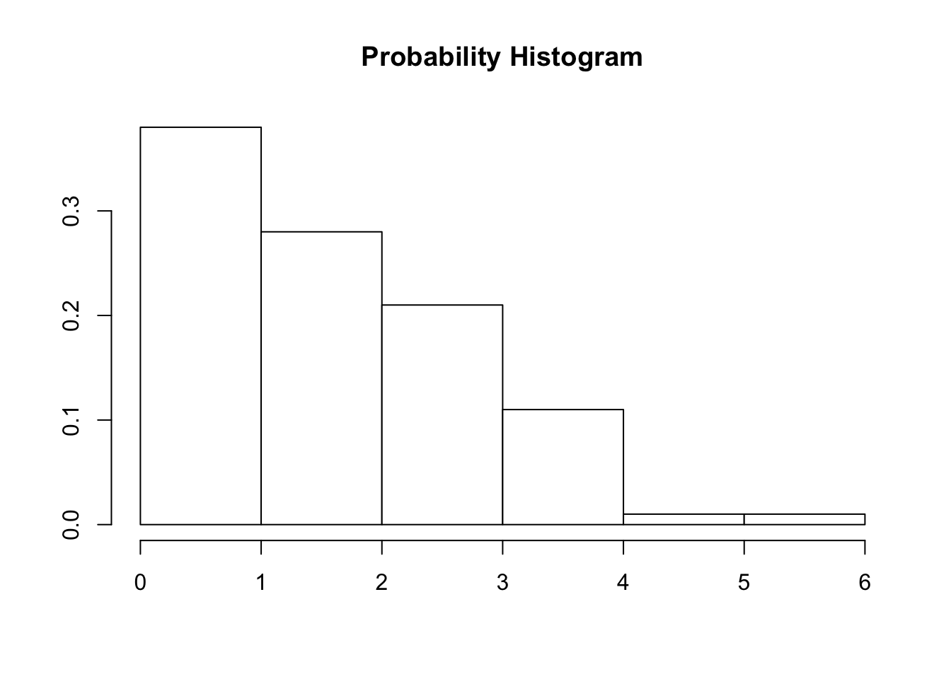
As with datasets, probability distributions can have shape and measures of center as well as spread
- What is the shape of this probability distribution?
Mean of a Discrete Probability Distribution
Mathematicians (and Statisticians) prefer deriving values and writing equations in more general forms
- Not because we like to confuse people, but because we’re lazy
We want to develop a general form for a measure of center and variability for a discrete probability distribution
Consider the probability distribution of \(X\) to be a population
Numerical values that we calculate from a probability distribution are called parameters
We would notate the mean of a population with \(\mu\)
- We can use the same notation for the mean of a probability distribution
Given several random variables to consider, we can denote the mean of r.v. \(X\) as:
\[\mu X \ \ \ \ \ \text{or} \ \ \ \ \ E(X)\]
For a discrete probability distribution of r.v. \(X\), the mean is given by:
\[E(X)=\mu=\sum_x xP(X=x)\]
- We call this “the weighted sum of all probabilities of \(x\)”
Mean of X Example
\(X=\{\text{number of customers in a line at the express checkout counter}\}\)
\[ \begin{array}{|c|c|c|c|c|c|c|} \hline x & 0 & 1 & 2 & 3 & 4 & 5 \\ \hline P(X = x) & 0.4 & 0.2 & 0.15 & 0.1 & 0.1 & 0.05 \\ \hline \end{array} \]
Recalling our definition of the mean of a probability distribution for a discrete r.v.
\[E(X)=\mu=\sum_x xP(X=x)\]
We get:
\[\mu_X=\sum_x xP(X=x)\] \[=0(0.4)+1(0.2)+2(0.15)+3(0.1)+4(0.1)+5(0.05)=1.45\]
- So we would say: “over time we expect to have \(1.45\) customers in a line at the express checkout counter”
Interpretation of the Mean of a r.v.
We’ve previously discussed how the mean of a dataset is it’s balance point (fulcrum)
- Shockingly, the exact same interpretation applies
You can also consider \(\mu\) to be the “average in the long run”
Using the Law of Large Numbers:
As we produce more observations and take their averages (\(\bar{x}\))
We should approach/converge on the value of \(\mu\)
Variance of a Discrete Probability Distribution
As discussed, probability distributions have spread, spread we can measure
Denoting the variance of discrete r.v. \(X\):
\[\sigma^2_X \ \ \ \ \ \text{or} \ \ \ \ \ Var(X)\]
The general formula for the variance of r.v. \(X\):
\[\sigma^2=\sum_x (x-\mu)^2 P(X=x)\]
Variance of X Example
\(X=\{\text{number of customers in a line at the express checkout counter}\}\)
\[ \begin{array}{|c|c|c|c|c|c|c|} \hline x & 0 & 1 & 2 & 3 & 4 & 5 \\ \hline P(X = x) & 0.4 & 0.2 & 0.15 & 0.1 & 0.1 & 0.05 \\ \hline \end{array} \]
Recalling our definition of variance:
\[\sigma^2=\sum_x (x-\mu)^2 P(X=x)\]
We get:
\[\sigma^2_X=\sum_x (x-\mu)^2 P(X=x), \ \ \ \text{recall} \ \mu=1.45\]
\[=(0-1.45)^2(0.4)+(1-1.45)^2(0.2)+(2-1.45)^2(0.15)+(3-1.45)^2(0.1)+(4-1.45)^2(0.1)+(5-1.45)^2(0.05)\]
\[=2.4475\]
For standard deviation, defined loosely as the “average” distance from \(\mu\) in the probability distribution:
\[\sigma=\sqrt{\sigma^2}\]
So:
\[\sigma_X=\sqrt{2.4475}\approx 1.564\]
In-class Exercise
Given the following probability distribution of discrete r.v. \(X\):
\[ \begin{array}{|c|c|c|c|c|} \hline x & 0 & 1 & 2 & 3 \\ \hline P(X = x) & 0.3 & 0.4 & 0.2 & 0.1 \\ \hline \end{array} \]
- Is this a proper probability distribution? Why or why not?
- Find \(E(X)\)
- Find \(Var(X)\)
- Find \(\sigma_X\)
Given the probability histogram for r.v. \(X\):
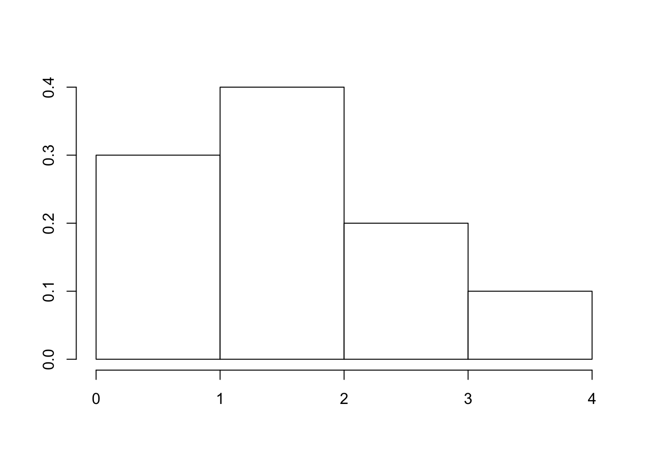
- What is it’s shape?
- Ok go away