18 Day 17

Review

Sampling Distribution

Given any population $Y \sim N(\mu,\sigma^2)$

• Sample $X \sim N(\mu_X,\sigma^2_X)$

• Sample mean $\bar{x} \sim N(\mu_{\bar{x}},\sigma^2_{\bar{x}})$

  • Where: $\mu_{\bar{x}} = \mu$

  • And: ${\sqrt{\sigma^2_{\bar{x}}}}=\sigma_{\bar{x}} = {\sigma \over \sqrt{n}}$

Central Limit Theorem

• Let $\bar{x}$ be the mean of a large random sample ($n > 30$) from any population

  • With mean $\mu$ and standard deviation $\sigma$

• The distribution of $\bar{x}$ is approximately normal

  • Mean $\mu_{\bar{x}} = \mu$

  • Standard deviation $\sigma_{\bar{x}} = \frac{\sigma}{\sqrt{n}}$.

If $n$ is large enough, we have:

$$\bar{x} \sim N(\mu, \frac{\sigma^2}{n})$$

• Regardless of the original population’s distribution

How large does $n$ need to be?

Population Proportion

• Proportions are just percentages of the population

• Say the percentage of the population who participate in early voting is $40\%$

  • ${40\over 100}=0.40$

  • The proportion of the population who early vote, $p=0.40$

• If we poll a sample of 100 Manhattan residents and find that $31\%$ early vote:

  • The proportion of our sample who early vote, $\hat{p}=0.31$

Just like every other statistic, sample proportions are random variables

• So their distribution is the sampling distribution of the proportion

All of our previous rules and ideas apply

• As we take samples from our population we will see they aren’t consistent

• The more we sample the closer we get to true values

• Mean of the sample proportion $\hat{p}$ is:

$$\mu_{\hat{p}} = p \quad \text{(population proportion)}$$

• Standard deviation of sample proportion $\hat{p}$ is:

$$\sigma_{\hat{p}} = \sqrt{\frac{p(1 - p)}{n}}$$

Proportion Central Limit Theorem

• If $np \geq 10$ and $n(1 - p) \geq 10$

• Distribution of $\hat{p}$ is approximately normal

  • Mean $\mu_{\hat{p}} = p$

  • Standard deviation $\sigma_{\hat{p}} = \sqrt{\frac{p(1 - p)}{n}}$

So:

$$\hat{p} \sim N \left( p, \frac{p(1 - p)}{n} \right)$$

• Point estimates are a deterministic result

  • Statistics deals with probabilistic results

Confidence Intervals

• Since: the value of $\bar{x}$ varies with each sample

  • We need to quantify the uncertainty associated with $\bar{x}$

  
  

Example:

A random sample of $120$ students admitted to top business schools yielded an average GPA of $3.45$

$$\bar{x} = 3.45$$ This is a point estimate of $\mu$

• One number, no additional information provided

A confidence interval (CI) provides a range of values that contains:

• The population parameter

• With a certain level of confidence

  • We refer to this as the confidence level

Formula for the CI:

$$\text{Point estimate} \pm \text{Margin of Error}$$

• The confidence interval for $\mu$:

$$\bar{x} \pm \text{Margin of Error}$$

$$(\bar{x} - \text{Margin of Error}, \bar{x} + \text{Margin of Error})$$

Margin of error

The farthest distance we believe our estimate $\bar{x}$ is from $\mu$

• The size of the margin of error is determined by the sampling distribution of $\bar{x}$ and the confidence level

• Confidence level is denoted by $100(1 - \alpha)\%$

  • Typically $90\%$, $95\%$, or $99\%$

For a population with unknown $\mu$ but known $\sigma$, a $100(1 - \alpha)\%$ confidence interval for $\mu$ is computed as:

$$\bar{x} \pm z_{\alpha/2} \cdot \frac{\sigma}{\sqrt{n}}$$

Where $z_{\alpha/2}$ is the z-score with an area of $\alpha/2$ to its right

When construction a confidence interval for $\mu$

• We have to consider our assumptions

At least one of the following must hold:

1. The sample size is large ($n > 30$)

2. The original population is normally distributed

In most practical cases, $\sigma$ is unknown, and we must use the sample standard deviation $s$

The formula for the confidence interval is:

$$\bar{x} \pm t_{\alpha/2} \cdot \frac{s}{\sqrt{n}}$$

Where $t_{\alpha/2}$ is the critical value from the Student’s t-distribution, and $s$ is the sample standard deviation

Student’s t-Distribution

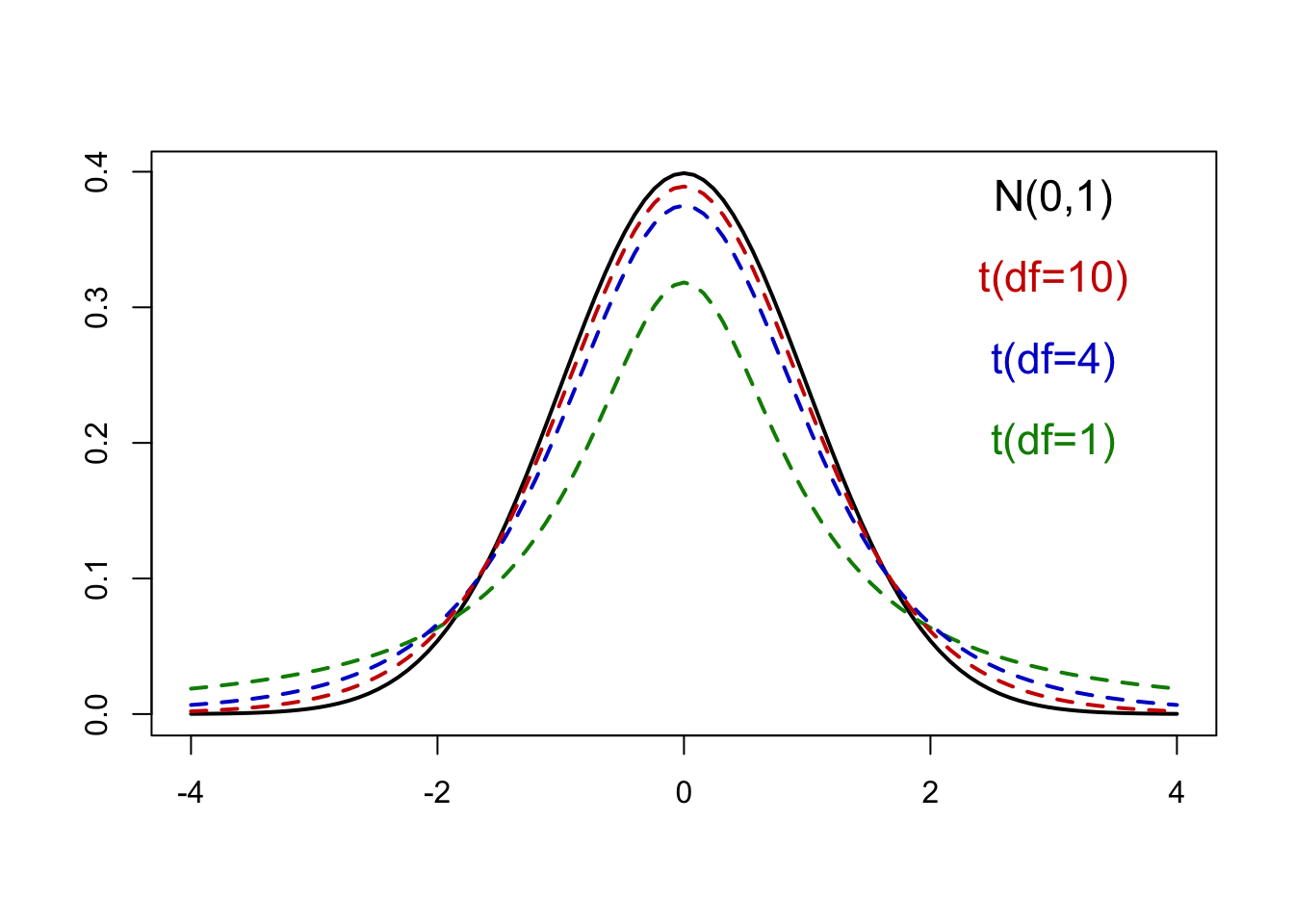
• The (Student’s) t-distribution is similar to the standard normal distribution

  • Unimodal

  • Symmetric around $0$

• But it has wider (or heavier) tails than the standard normal

  • Meaning it’s more spread out

• The t-distribution is distinguished by degrees of freedom ($df = n - 1$)

  • As $df$ increase the t-distribution converges to a normal distribution

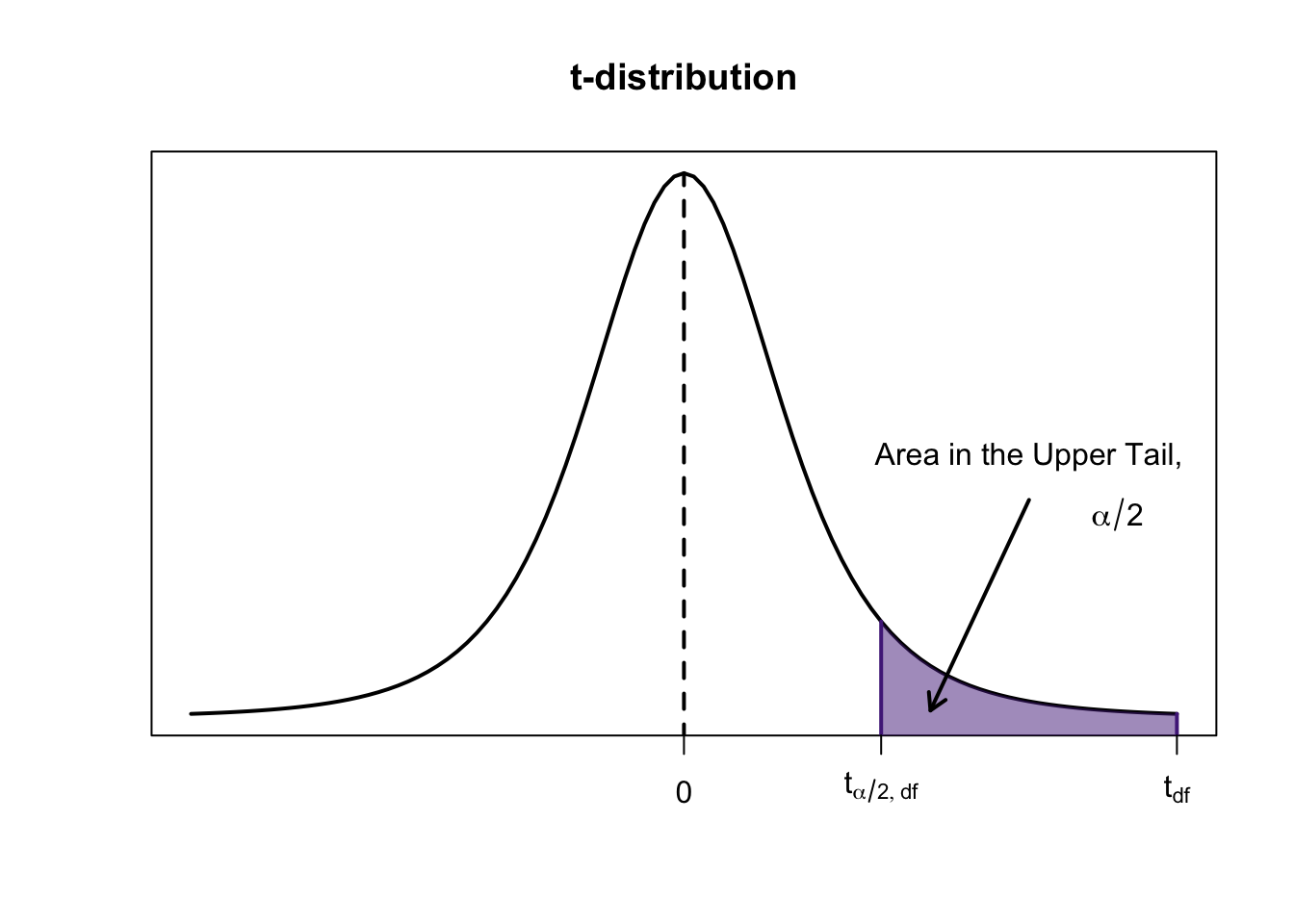
The critical value $t_{\alpha/2}$ is a $t$ value separating an area of $\alpha/2$ in the right tail of the $t$ distribution

When using the $t$ distribution ot construct a confidence interval for $\mu$:

• Degrees of freedom ($df$) is $1$ less than the sample size

Example 1: Finding Critical Value

Find the critical value $t_{\alpha/2}$ for a 95% confidence interval with $n = 8$

• Set $1 - \alpha = 0.95$, then $\alpha = 0.05$, and $\alpha/2 = 0.025$

• For $n = 8 \Rightarrow df = n-1 = 7$

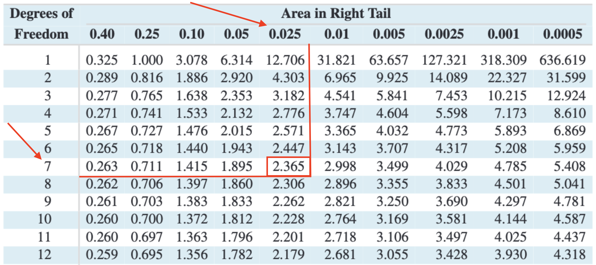
The critical value is $t_{\alpha/2} = 2.365$

What is the $df$ I’m looking for isn’t in the table?

• Round down to the nearest value on the table

  • If $df=59$, round down to $df=50$

  • At $95\%$ confidence, $t_{\alpha/2}=2.009$

Summary of CI for Population Mean $\mu$:

Check your assumptions for construction a CI of $\mu$:

• Sample size is large ($n>30$) or the population is normal

$100(1-\alpha)\%$ confidence interval is computed as:

• Case 1: $\sigma$ is known, use the z-method:

  $$\bar{x} \pm z_{\alpha/2} \cdot \frac{\sigma}{\sqrt{n}}$$

• Case 2: $\sigma$ is unknown, use the t-method:

  $$\bar{x} \pm t_{\alpha/2} \cdot \frac{s}{\sqrt{n}}$$

Example 2: Constructing a CI

Given a sample of size $n = 5$ from a normal population, $\bar{x} = 4.31$, and $s = 2.7$, construct a 95% confidence interval for $\mu$

1. Should we use $z$ method or $t$ method?

• $\sigma$ is unknown

2. Compute the margin of error for this $95\%$ confidence interval:

• With $df = 4$ and $t_{\alpha/2} = 2.776$, calculate:

$$\text{Margin of Error} = 2.776 \times \frac{2.7}{\sqrt{5}} \approx 3.352$$

3. Construct a $95\%$ confidence interval for $\mu$ and interpret your result:

$$4.31 \pm 3.352 \quad \text{or} \quad (0.958, 7.662)$$

We are 95% confident that the true population mean lies between 0.958 and 7.662

4. If the population were not normal, would the confidence interval in (c) be valid?

Interpreting a CI

• Suppose we take many random samples and construct a $95\%$ confidence interval from each sample

  • $95\%$ of those intervals would contain the true population mean, $\mu$

In practice:

• We say that we’re $95\%$ confident that the true value of $\mu$ is within our confidence interval