6 Day 5
Announcements:
Stat Help Lab:
- Monday - Friday \(\approx\) 9 AM - 6 PM
Homework point recovery
I’m writing this August 31
Hopefully past me has graded them
- He did
Question 5 - Qualitative vs Quantitative
Supplemental materials
Extracurricular materials
Review
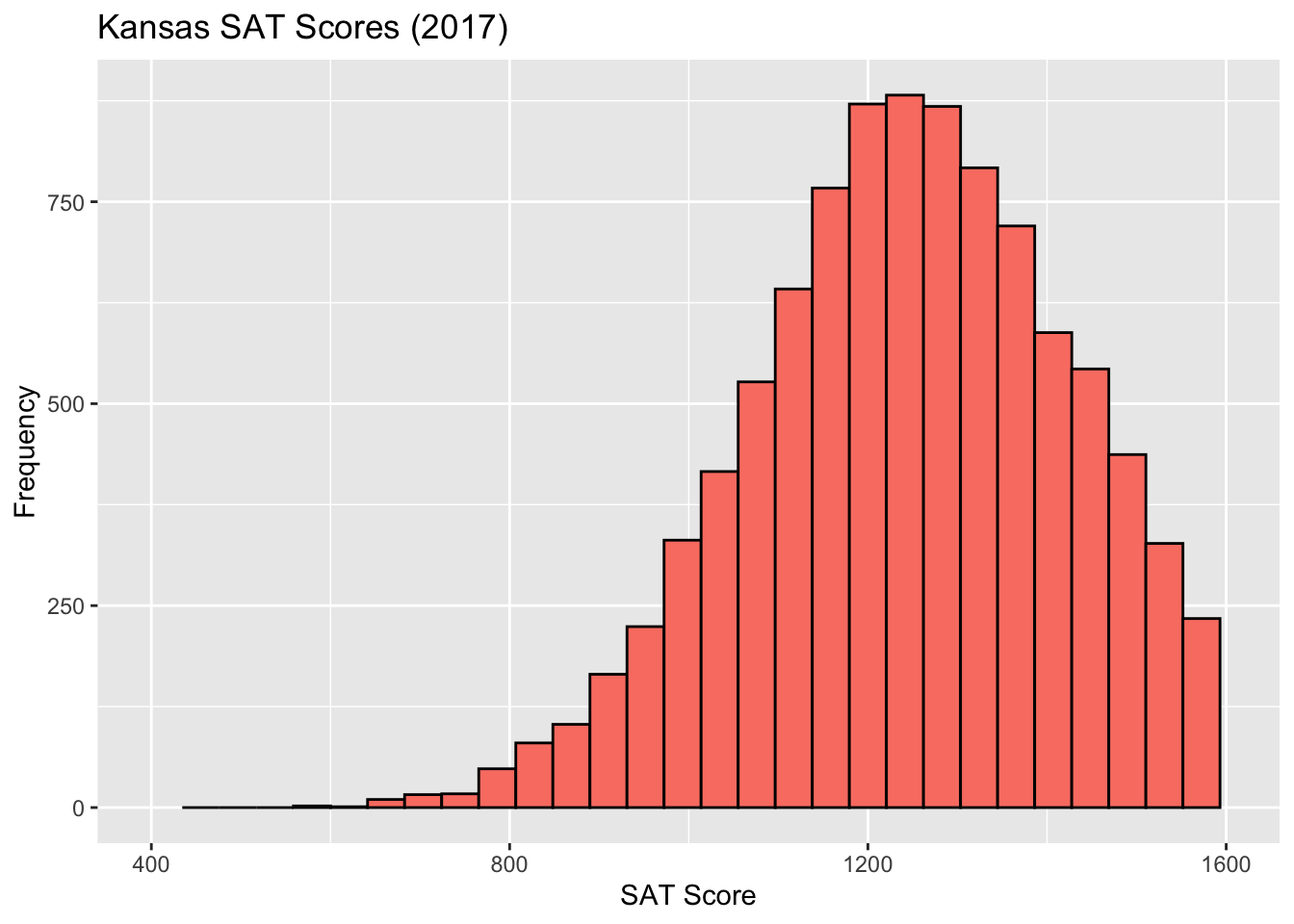
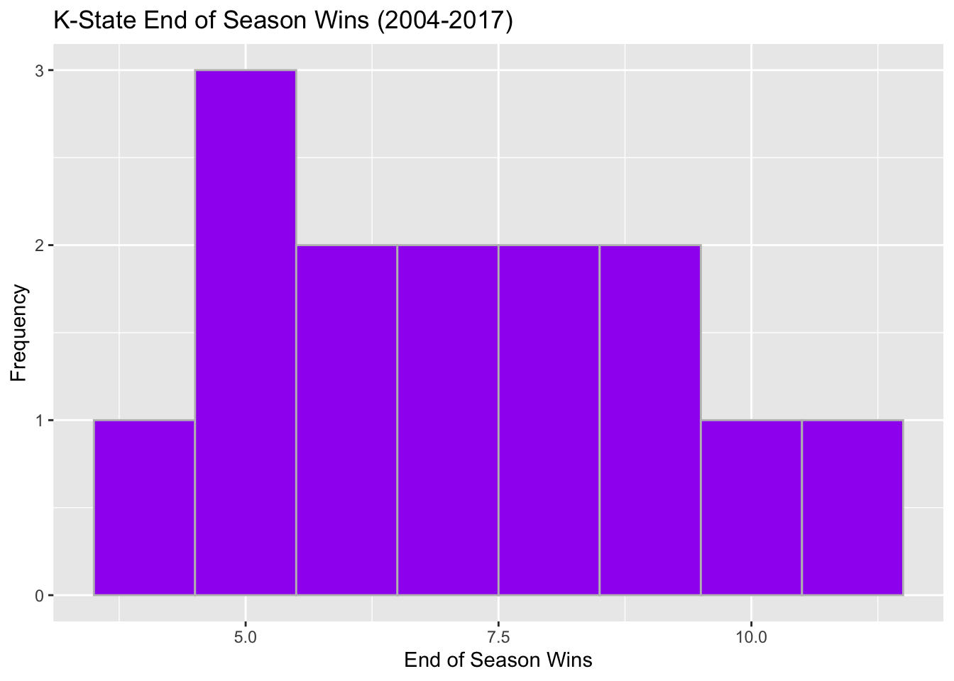
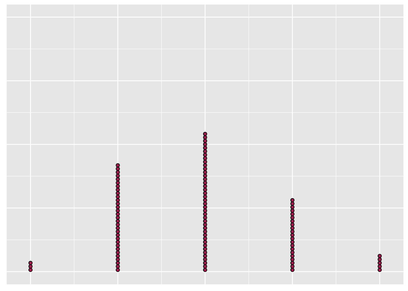
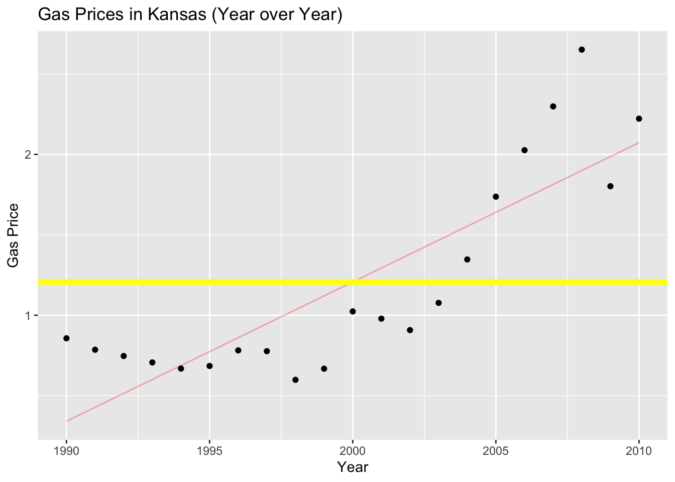
Which way is this histogram skewed?
Numerical summaries help us understand data sets faster
Notation is how we communicate statistical/mathematical equations:
Sample size (# of individuals in a sample)
- Denoted with \(n\) (lower-case)
Population size
- Denoted with \(N\) (capital)
Data values can be denoted as \(x_1,x_2,x_3,...\)
\(x_1\) refers to the observed value of the variable \(x\) from individual 1
Summation:
This is referring to the sum (addition) of everything contained in the expression
We denote this with the Greek letter \(\Sigma\)
\[\sum\limits_{i=1}^nx_i=x_1+x_2+...+x_n\]
Mean
Balance point (fulcrum) of the dataset
Population mean (denoted \(\mu\)):
\[\mu = {1 \over N}\sum\limits_{i=1}^Nx_i\] \[\mu = {\sum\limits_{i=1}^Nx_i\over N}\]
\[N \approx 10000\]
\[\mu = {1 \over 10000}(x_1 + x_2 +x_3 + ...+x_{10000})\]
\[\mu = 1258.771\]
- Is \(\mu\) a statistic?
| 1149 | 1577 | 1138 | 1319 | 1399 | 1074 | 1091 | 1324 | 1048 | 1462 |
\[\bar{x} = {1 \over n}\sum\limits_{i=1}^nx_i\]
\[\bar{x} = {\sum\limits_{i=1}^nx_i\over n}\]
Properties of mean:
Common
Easy to interpret
Susceptible to outliers
A statistic is resistant if its value is not affected heavily by outliers
Median
- Half of the data points are above the median, half are below
| 1149 | 1577 | 1138 | 1319 | 1399 | 1074 | 1091 | 1324 | 1048 | 1462 |
- Sort your data in increasing order (low to high)
| 1048 | 1074 | 1091 | 1138 | 1149 | 1319 | 1324 | 1399 | 1462 | 1577 |
If \(n\) is odd: choose position \({(n+1)\over2}\) in the ordered dataset
If \(n\) is even after ordering:
Pick \(n\over 2\) and \({n \over 2}+1\)
Average the two data points
\[{10\over2}=5 \ , \ {10 \over2}+1=6\] \[{\ \ \ + \ \ \ \over2}= \ \ \]
Properties of median:
It doesn’t use all of the data directly
This makes it resistant
- Outliers have little/no effect
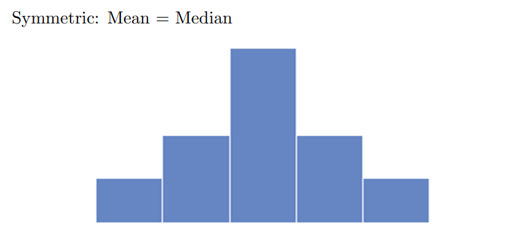
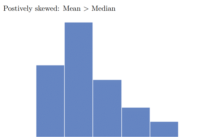
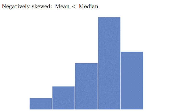
Difference between median and mean depend on skew of the histogram
Mode
Where the peak is
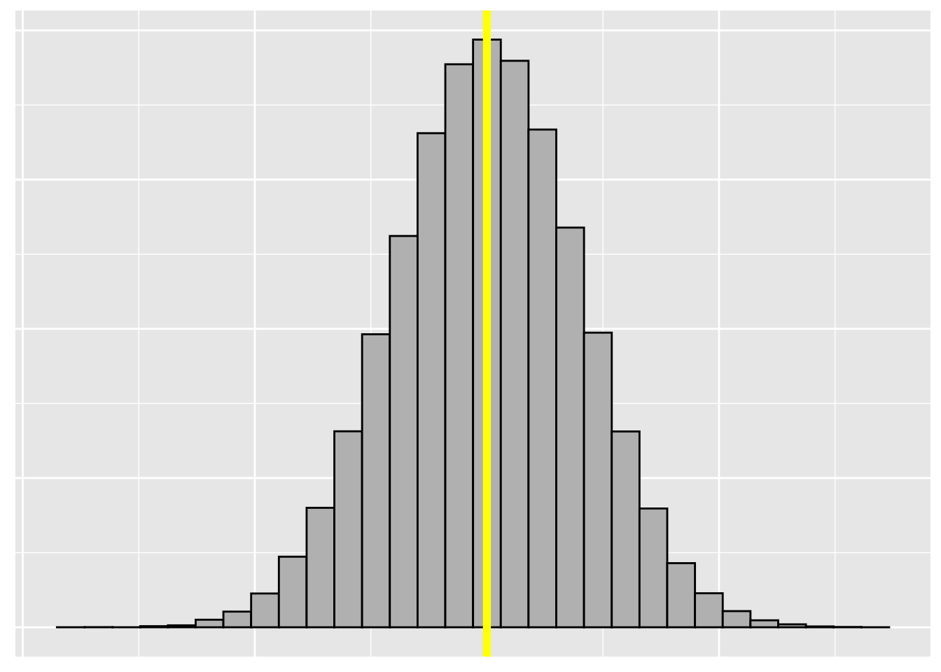
What could be the mode here?

The most frequent observation
Useful for qualitative data
- “Which credit card is most commonly used by our customers?”
Not as useful for quantitative data
- “What’s the most common weight of cattle on our research farms?”
A data set can have any number of modes (0,1,2,…)
| V1 | 8 | 10 | 7 | 11 | 14 | 12 | 11 | 9 | 14 | 11 | 8 | 2 | 8 | 10 | 7 | 12 | 11 | 12 | 12 | 10 |
| V2 | 5 | 13 | 15 | 9 | 10 | 13 | 16 | 11 | 13 | 11 | 7 | 15 | 10 | 16 | 11 | 18 | 13 | 10 | 9 | 9 |
Whatever method works best for you is the one you use
Personally, I prefer to make a frequency table:
| Value | Freq |
|---|---|
| 2 | 1 |
| 5 | 1 |
| 7 | 3 |
| 8 | 3 |
| 9 | 4 |
| 10 | 6 |
| 11 | 7 |
| 12 | 4 |
| 13 | 4 |
| 14 | 2 |
| 15 | 2 |
| 16 | 2 |
| 18 | 1 |
Measures of Spread
Statistics is roughly about making inference from data
Is it fair to make inference from mean/median/mode alone?
Is the mean resistant?
Is the median representative of all the data?
Does the mode tell us about outliers?
When we look at data there’s a certain spread to it:
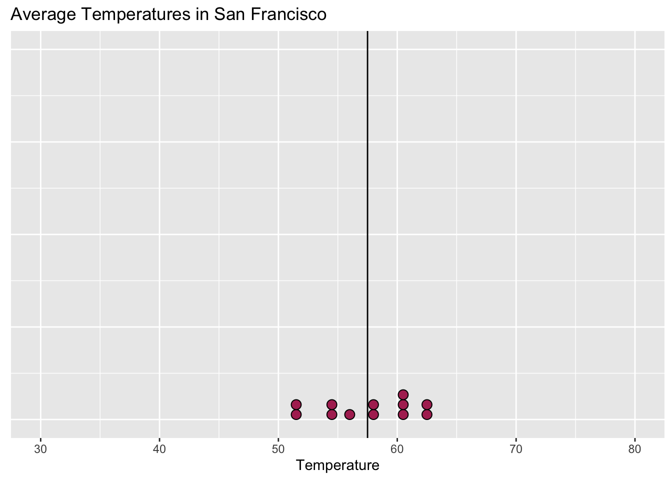
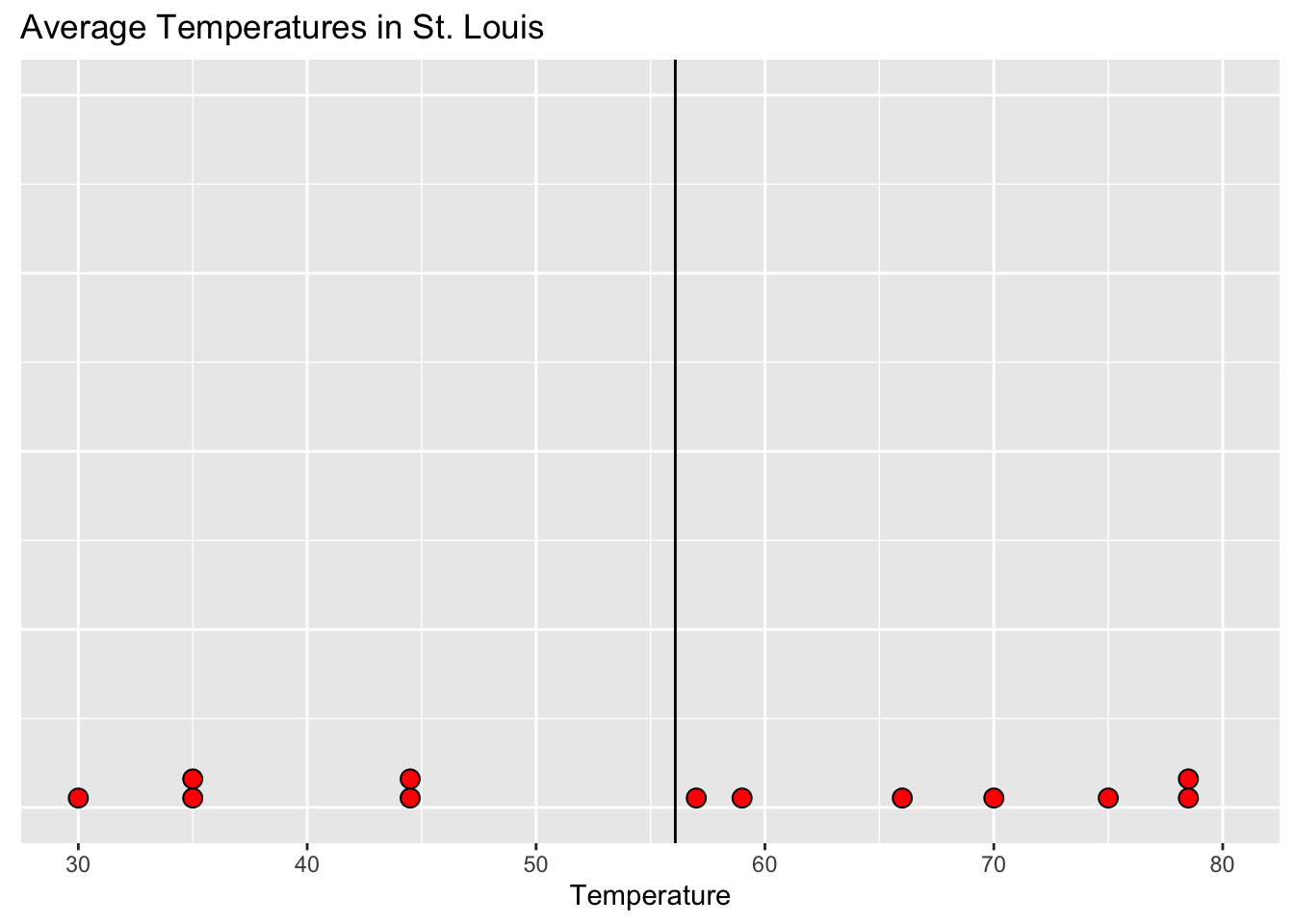
| Months | Jan | Feb | Mar | Apr | May | Jun | Jul | Aug | Sep | Oct | Nov | Dec |
| San Francisco | 51 | 54 | 55 | 56 | 58 | 60 | 60 | 61 | 63 | 62 | 58 | 52 |
| St. Louis | 30 | 35 | 44 | 57 | 66 | 75 | 79 | 78 | 70 | 59 | 45 | 35 |
\[\mu_{sf} = {{51+54+55+56+58+60+60+61+63+62+58+52}\over 12} = 57.5\]
\[\mu_{sl} = {{30+35+44+57+66+75+79+78+70+59+45+35}\over 12} = 56.1\] - The means are similar
Are the temperatures in each city similar?
- Common sense: Who’s been to San Francisco?
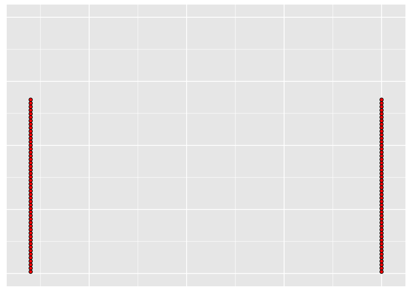
Note: The program I use to make this is bad at dotplots
- There’s a reason for that
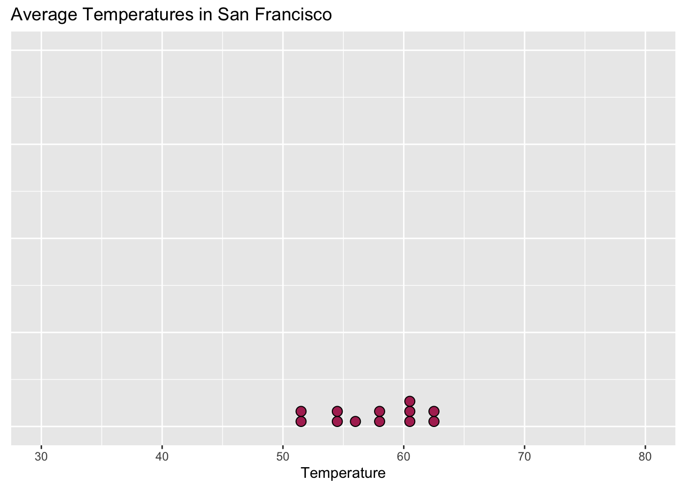
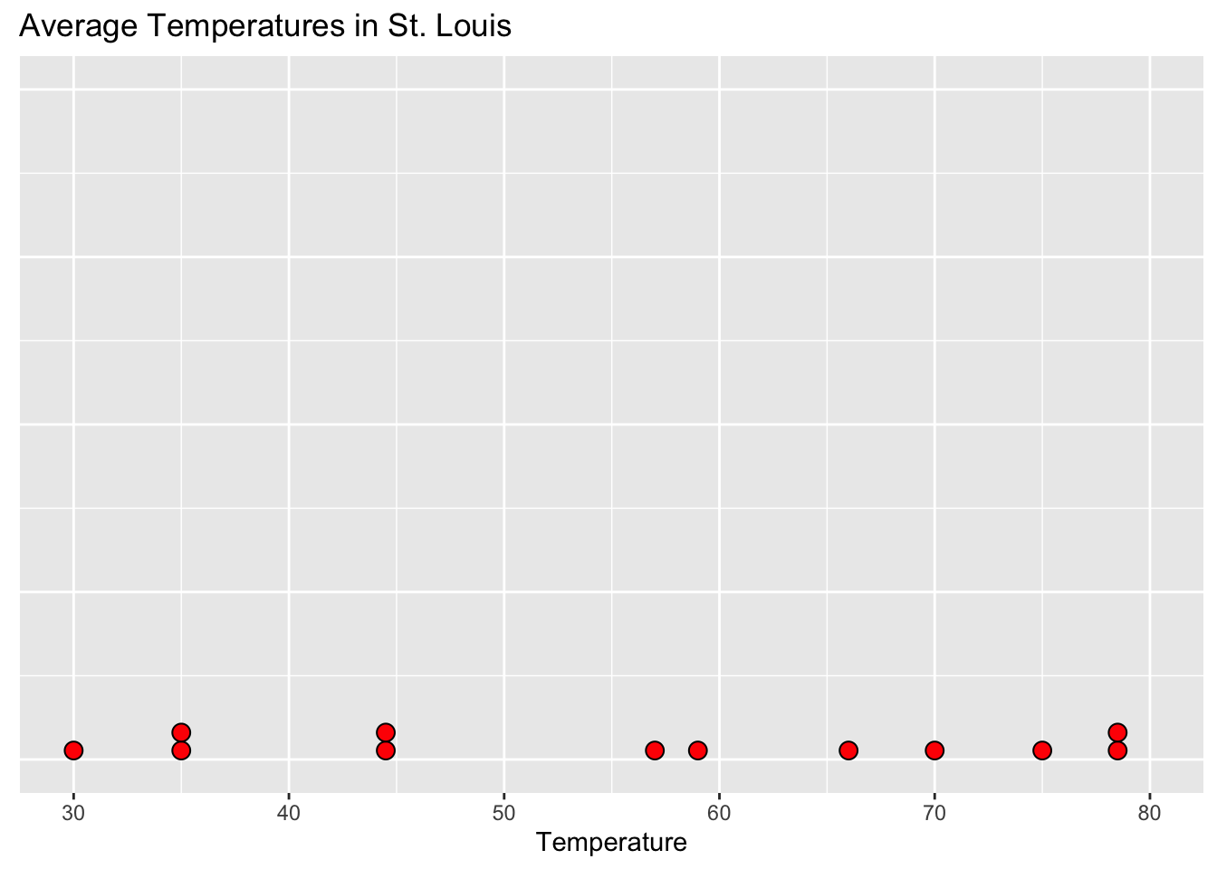
Are they different?
- In what way?
Spread is an important metric for understanding the differences or variation in data
Range
Simplest measure of spread
Difference between the largest and smallest data value
\[Range = Max - Min\]
| Months | Jan | Feb | Mar | Apr | May | Jun | Jul | Aug | Sep | Oct | Nov | Dec |
| San Francisco | 51 | 54 | 55 | 56 | 58 | 60 | 60 | 61 | 63 | 62 | 58 | 52 |
| St. Louis | 30 | 35 | 44 | 57 | 66 | 75 | 79 | 78 | 70 | 59 | 45 | 35 |
- Calculate the range of both San Francisco and St. Louis in this data set
What do our results mean?
With every measure/metric there’s good and bad
Range does let us look at spread
- It uses two values so it’s not a perfect measure
These two data sets could have the same range and mean
- Are they the same data set if that’s true?
- Smaller spread is usually closer to the mean
- Larger spread is usually further from the mean
Variance
Measure of how far, on average, values in a data set are from the mean
- Population mean (denoted \(\mu\)):
\[\mu = {1 \over N}\sum\limits_{i=1}^Nx_i\]
\[\mu = {\sum\limits_{i=1}^Nx_i\over N}\]
- Sample mean (denoted \(\bar{x}\))
\[\bar{x} = {1 \over n}\sum\limits_{i=1}^nx_i\]
\[\bar{x} = {\sum\limits_{i=1}^nx_i\over n}\]
Stay with me
Let \(x_1,x_2,...,x_N\) be values in a population of \(N\) size
The difference between \(i^{th}\) population value and the mean is:
\[x_i - \mu\]
We want to take these differences from \(1\) to \(i\) and divide them by \(N\)
There’s one problem though:
Positive and negative difference can cancel out
We can fix that by squaring the value of each difference:
\[(x_i - \mu)^2\]
Given this:
Variance should never be negative
Zero or positive
Larger variance means more variability
- Population variance (denoted \(\sigma^2\)):
\[\sigma^2 = {{{\sum\limits_{i=1}^N}(x_i-\mu)^2}\over N}\]
- Sample variance (denoted \(s^2\)):
\[s^2 = {{{\sum\limits_{i=1}^n}(x_i-\bar{x})^2}\over (n-1)}\]
Remember that statistics is roughly:
- Making inference about a population parameter using sample statistics
In practice we almost never have a population variance
- We use a sample variance to estimate population variance
Practice: Calculate Sample Variance
A company that manufactures batteries is testing a new type of battery designed for laptop computers. They measure the lifetimes, in hours, of six batteries, and the results are 3, 4, 6, 5, 4, and 2. Find the sample variance, including its unit, of the lifetimes
Standard Deviation
Variance is a squared unit of the data
- It’s annoying to think in squares

The value of variance we calculated in the previous example is “\(Hours^2\)”
This is an easy fix though:
\[\sqrt{Hours^2}=Hours\] - We call this standard deviation
It lets us work in the original units of the data
The notation is easy to understand as well
\[\sqrt{\sigma^2}=\sigma \rightarrow Population \ Standard \ Deviation\]
\[\sqrt{s^2}=s \rightarrow Sample \ Standard \ Deviation\]
In our previous practice example we calculated a variance in \(Hours^2\)
- What is the standard deviation in hours?
| Battery | A | B | C | D | E | F |
| Lifespan | 3 | 4 | 6 | 5 | 4 | 2 |
Practice: Mean, Variance, and Standard Deviation
| 17 | 40 | 24 | 18 | 16 |
Compute:
Sample Mean
Sample Variance
Sample Standard Deviation
| 1149 | 1577 | 1138 | 1319 | 1399 | 1074 | 1091 | 1324 | 1048 | 1462 |
Compute:
Sample Range
Sample Standard Deviation
The population standard deviation of this data is \(188\)
- What do you make of the sample standard deviation you computed?
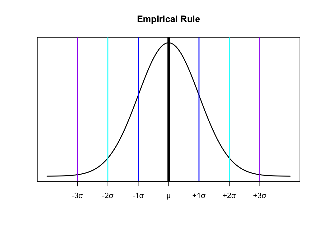
Empirical Rule
Many data sets has a single peak in the center and an approximately symmetric shape
- We call this a bell-shape
When we see this distribution we can use standard deviation to describe how much of the data is within a certain range of the mean
The Empirical Rule
For a population that has an approximately bell-shaped distribution:
\(\approx 68\%\) of the data is within ONE standard deviation of the mean
\[\approx 68\% = \begin{cases} \mu - \sigma \\ \mu + \sigma \end{cases}\]
- \(\approx 95\%\)$ of the data is within TWO standard deviations of the mean
\[\approx 95\% = \begin{cases} \mu - 2\sigma \\ \mu + 2\sigma \end{cases}\]
- \(\approx\) All or almost all of the data is within THREE standard deviations of the mean
\[\approx 100\% = \begin{cases} \mu - 3\sigma \\ \mu + 3\sigma \end{cases}\]
Practice: Empirical Rule
A large class of 200 students took an exam. The scores had sample mean \(\bar{x} = 65\) and sample standard deviation \(s = 10\). The histogram is approximately bell-shaped.
Find an interval that is likely to contain approximately 68% of the scores.
Approximately what percentage of the scores were between 45 and 85?
Approximately how many students had scores between 45 and 85?
- Go away
Extracurricular
I promised I’d explain the Kansas SAT test scores histogram:
set.seed(80)
empir_rule <- data.frame(x = rnorm(200,65,10))

ggplot(data=empir_rule,aes(x=x)) + geom_histogram(stat="bin",binwidth=6,color="black",fill="violet") +
labs(x="Student Exam Scores",y="Frequency",title="Empirical Rule Example")![]()
Mean and standard deviation/variance of a sample/population can be used to simulate the data
Ideally you know the shape of the data too
Since I know this is approximately bell shaped:
- I can make fake data using the sample statistics