16 Day 15

Announcements

• Don’t come to class sick

  • Don’t come to class sick

    • Don’t come to class sick

• If you miss class, review the notes

  • If you have questions on the notes please email me

    • Whatever confused you definitely confused someone else, you’re helping me as an instructor more than yourself. There are no stupid questions.

• Today is a day about conceptual knowledge

  • Just try to focus on understanding the theory rather than the math

Review

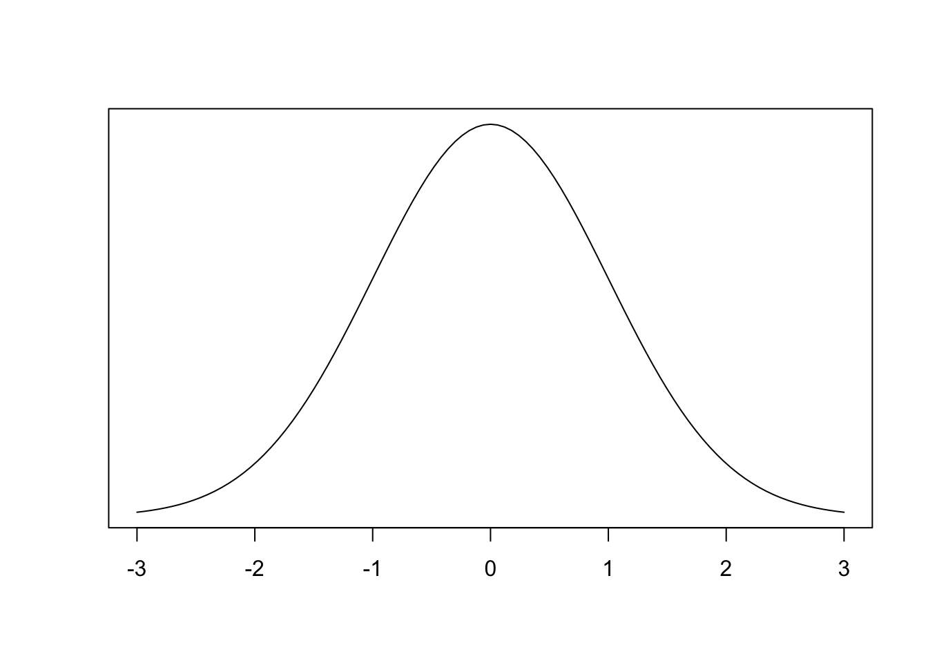
A standard normal distribution is a normal distribution with:

• $\mu=0$

• $\sigma = 1$

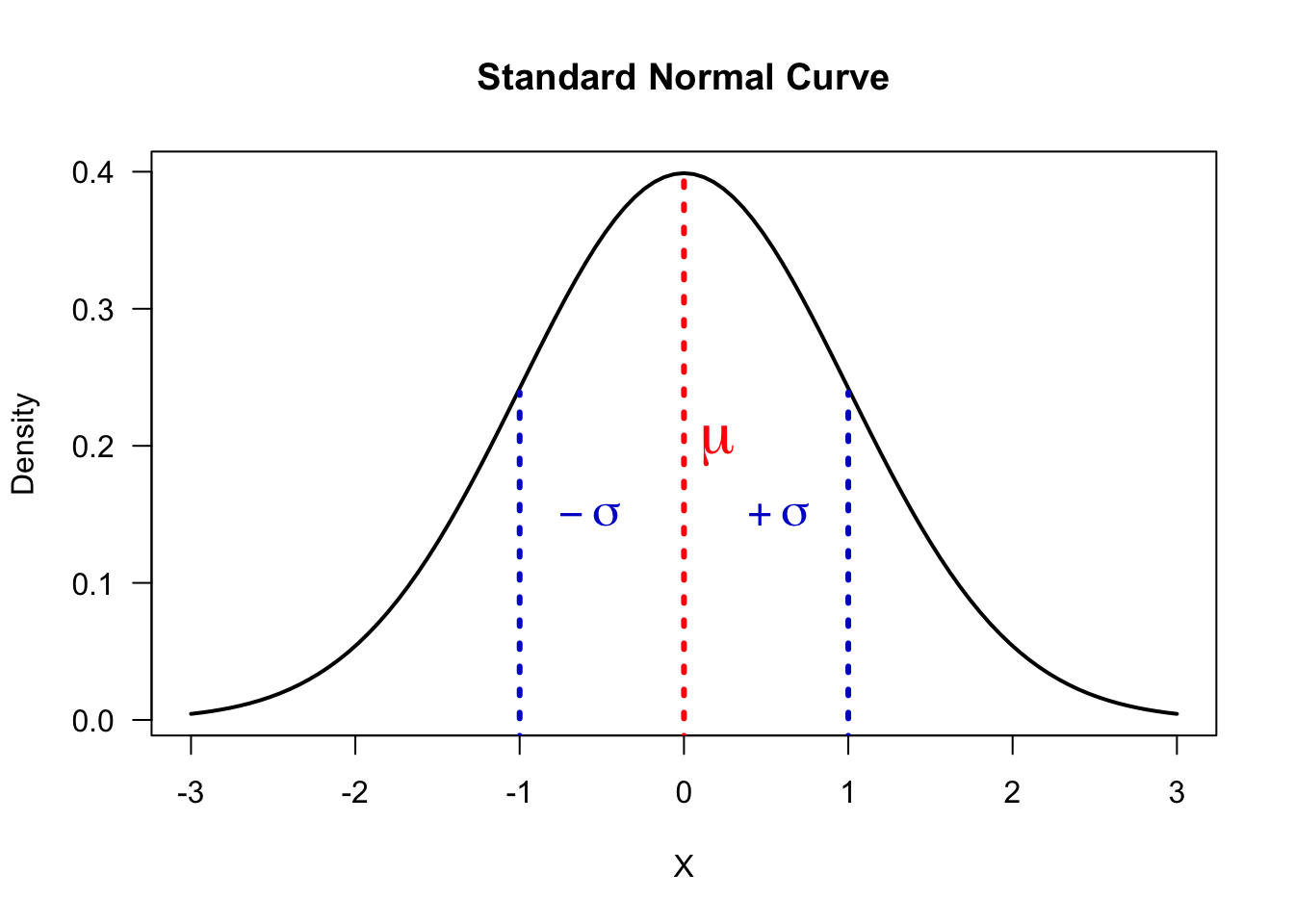
We use the letter $Z$ to represent a standard normal random variable (referring to $z$-score)

The probability that a standard normal random variable $Z$ is between $a$ and $b$ ($P(a<Z<b)$) is equal to the area under the standard normal curve over the interval $[a,b]$

To make inference about the standard Normal distribution, for this class we use the $z$-table

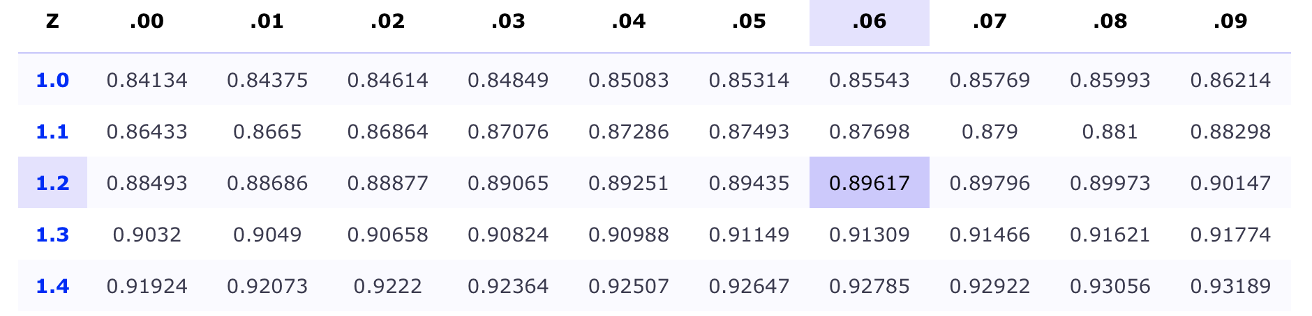
• Reading it isn’t difficult

• You can put a reminder on your cheat sheet if you so choose:

$$\text{Left Column}=0.0X, \ i.e. 1.2X$$

$$\text{Top Column}=X.X0, \ i.e. X.X6$$

$$L+T=1.26$$

The difficulty is getting to the point where we read it

• Conceptually you need to grasp a couple things:

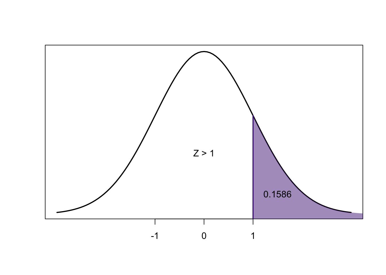
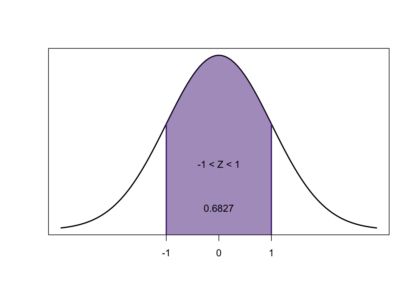
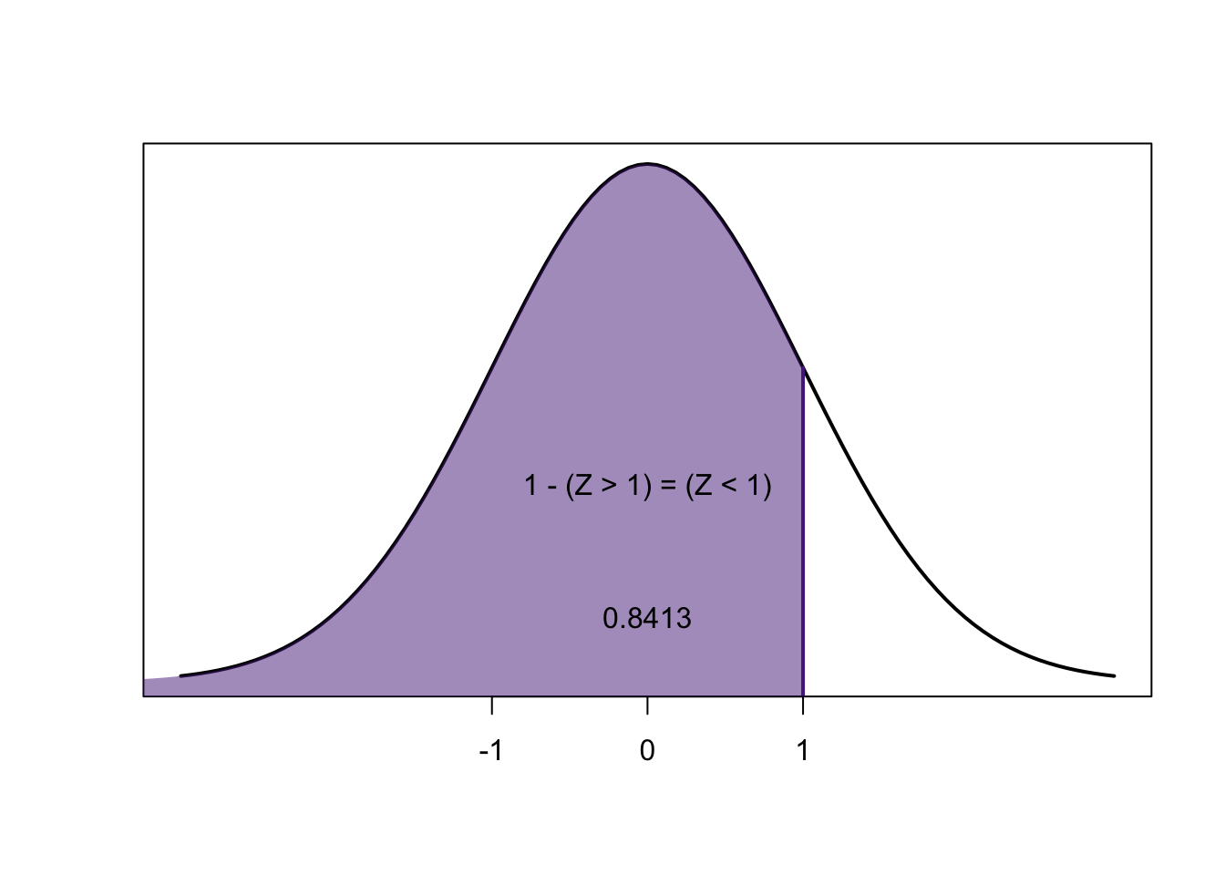
$$0.8413-0.1586=0.6827$$

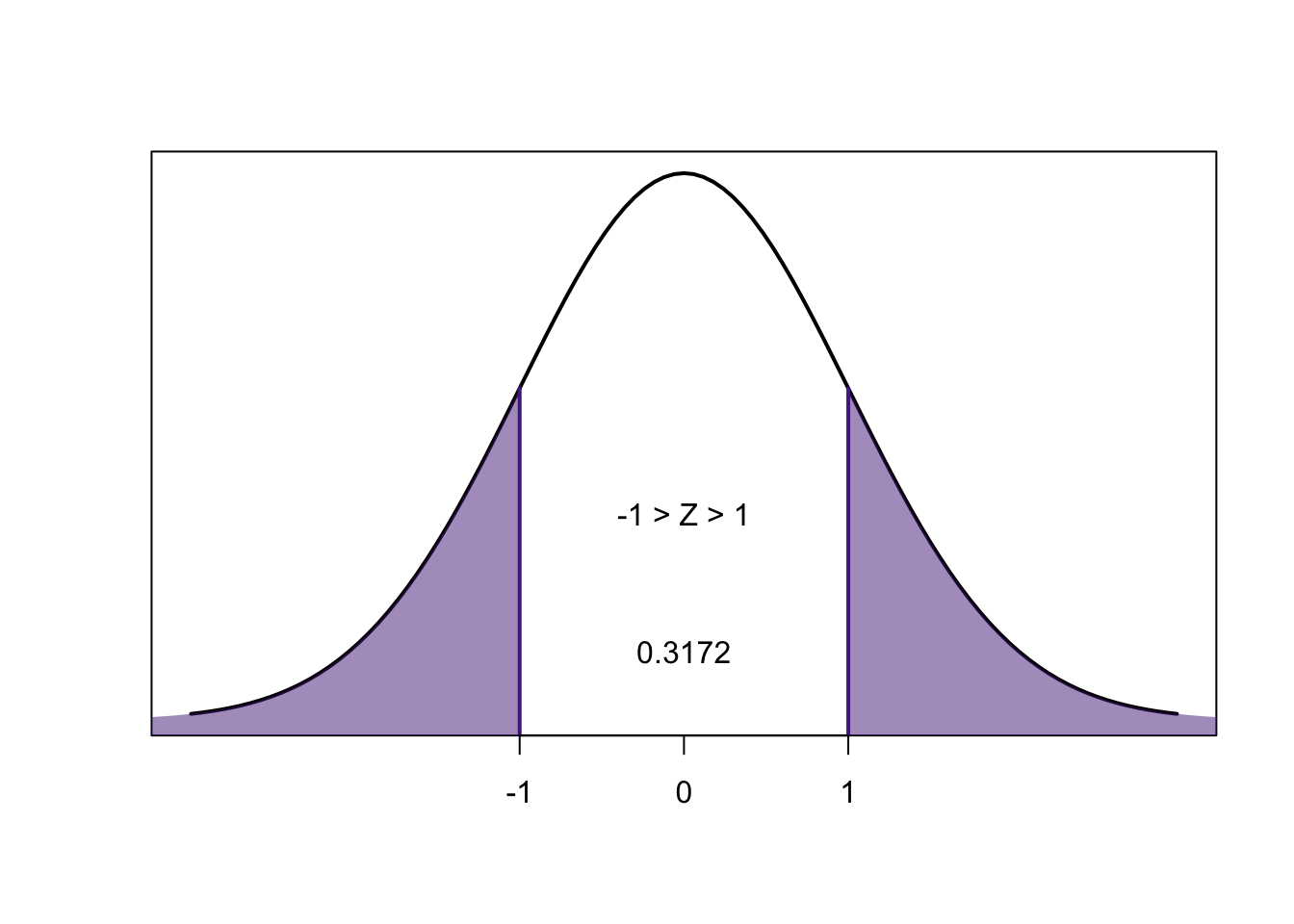
$$1-0.6827=0.3173$$

A tool for your toolbox

$$1-0.1586=0.8414 \newline 0.8414-0.1586=0.6828$$

What have we done?

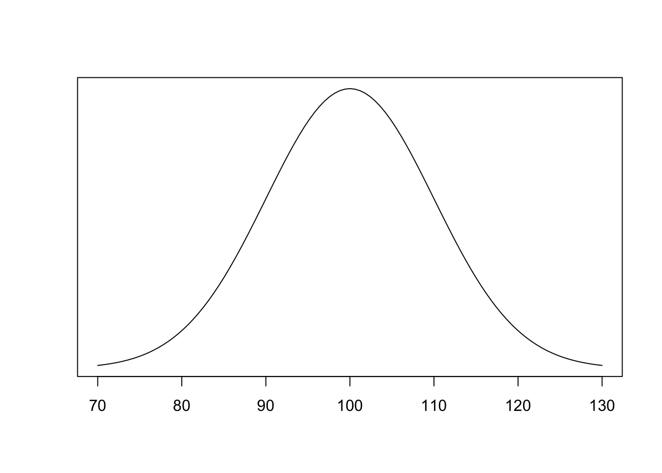
Non-standard Normal Distributions

If $X$ is a normal random variable with mean $\mu$ and standard deviation $\sigma$ we write $X \sim N(\mu,\sigma^2)$

• $\sim$ means “is distributed (as)”

• $N()$ refers to the normal distribution

  • Together we’re saying “X is distributed normal with mean $\mu$ and variance $\sigma^2$

• So if $\mu=100$ and $\sigma=5$ we’ll write $X\sim (100,5^2)$ or $X \sim (100,25)$

• If we write $X \sim (16,5)$ then $\mu=16$ and $\sigma=\sqrt{5}$

We’ve seen that the standard normal distribution is well understood and we can find probabilities, percentiles, etc. “easily” using a $z$-table

If we want to easily learn these things about non-standard random variables it would be convenient if we could transform them into standard normal random variables

• Fortunately we can

$$\text{if} \ X \sim N(\mu,\sigma^2), \ \text{then} \ Z={X-\mu \over \sigma} \sim N(0,1)$$

$$X \sim N(100,10) \Rightarrow Z={X-100 \over 10} \sim N(0,1)$$

$$z={x-\mu \over \sigma}$$

What we’ve done is convert the non-standard normal distribution into a set of $z$-scores

• What do these $z$-scores measure?

The process we’ve performed in making this conversion is called standardizing a normal random variable

• We can do this moving forward to find out information from a non-standard normal r.v. using the $z$-tables

$$P(X\leq x)=P\left({X-\mu \over \sigma}\leq{x-\mu \over \sigma}\right)=P(Z\leq z)$$

Non-standard Normal Examples

Suppose that the heights of American men ($20$ years and older) are approximately normal with a mean of $70$ inches and a standard deviation of $4$ inches.

1. What proportion of American men are less than $6$ feet tall?

• ($6$’ $=$ $72$”)

• $X \sim N(70,4^2)$

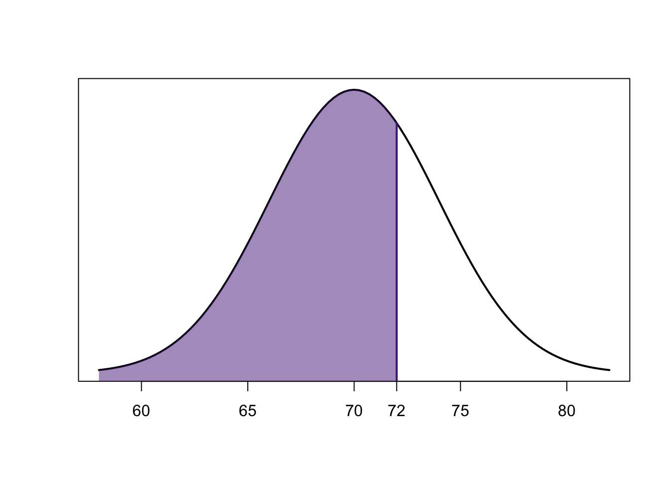
$$P(X\leq 72)=P\left(Z\leq{72-70 \over 4}\right)=P(Z\leq 0.5)$$

2. What proportion of American men are between 5’ and 6’ 8”tall?

• ($5$’$=$ $60$” and $6$’$8$” $=$ $80$”)

$$P(60<X<80)=P\left({60-70 \over 4}<Z<{80-70 \over 4}\right)$$

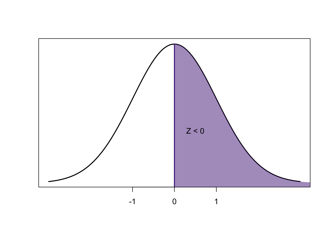
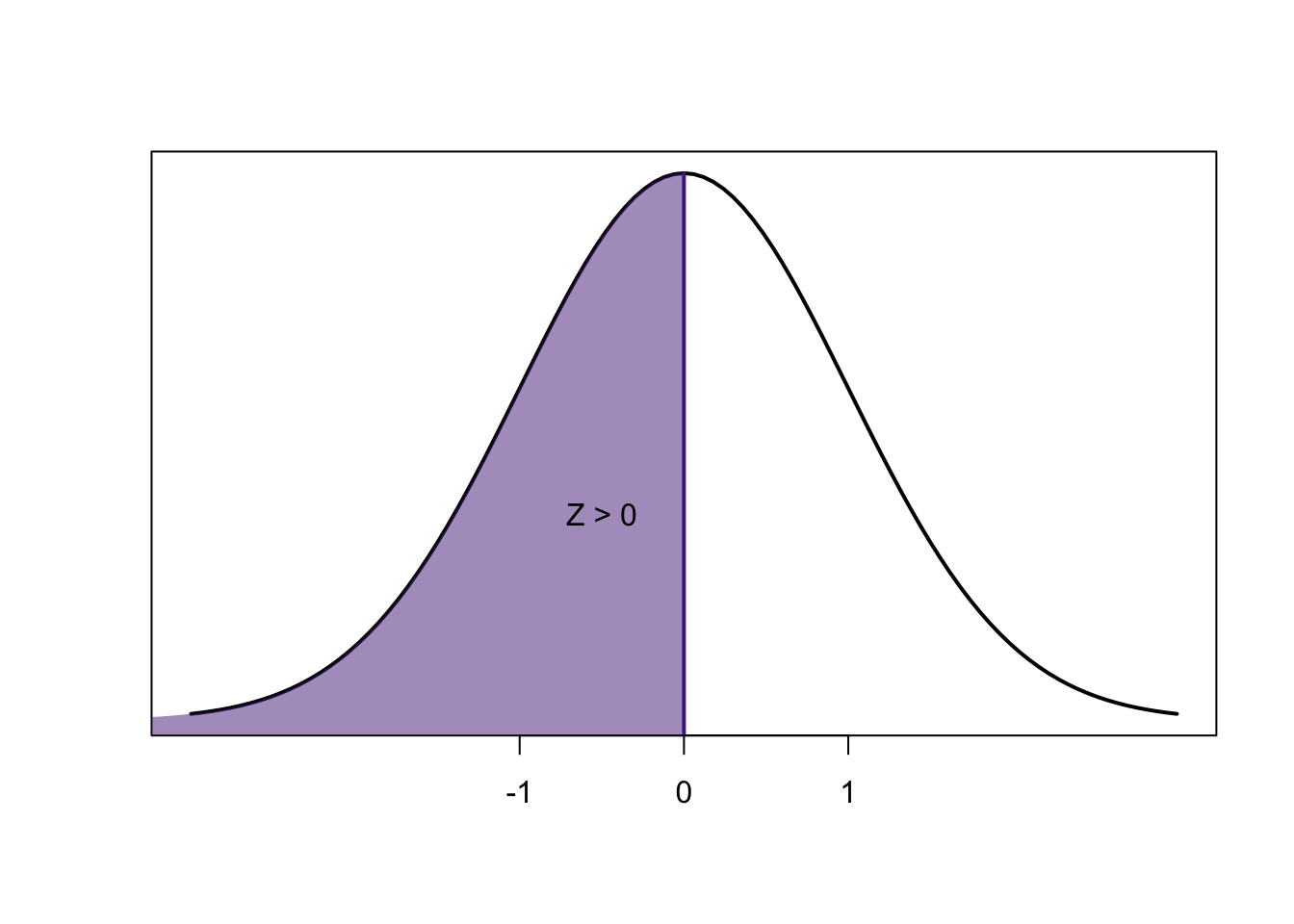
We know that for any $z$-score, the area to the left of the negative is exactly equal to the area to the right of the positive:

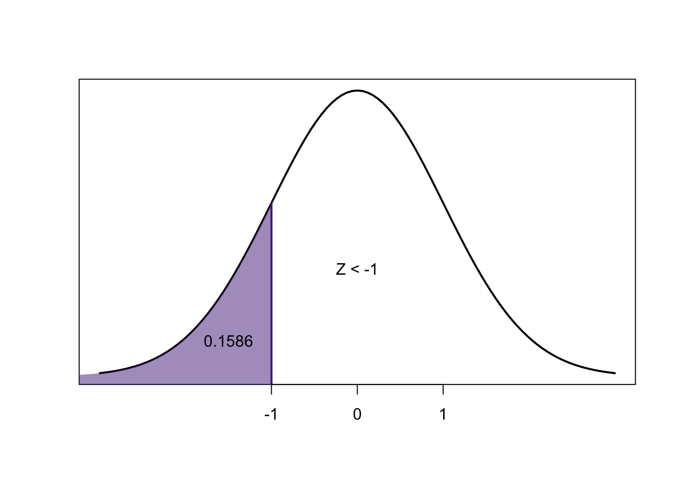
So:

$$=P(-2.50<Z<2.50) =2\times P(Z<-2.50)$$

$$=1-2(\ \ \ \ \ \ \ \ \ \ \ \ \ \ \ \ \ \ \ \ \ )=$$

Given our height example ($X \sim N(70,4^2)$), how tall would you have to be so that you are taller than $90\%$ of American men?

• Refer to your $z$-table

  • Find the closest value to $0.90$

  • “un-standardize” the value:

$$x=\sigma z + \mu=4( \ \ \ \ \ \ \ \ \ \ \ \ \ ) + 70 =$$

What is an interval of two heights that contains approximately $50\%$ of American men?

• Find a value on your $z$-table that is approximately $0.25$ or $0.75$

  • Why these values?

• We should end up with $0.67$ at $0.75$

  • at $0.25$ it should be $-0.67$

$$x=\sigma (-z) + \mu=4(-0.67) + 70 =67.32$$

$$x=\sigma z + \mu=4(0.67) + 70 =72.68$$

Sampling Distribution of Sample Mean & Central Limit

Let’s remember some core vocabulary:

• Population: The entire collection of individuals we’re seeking information from

• Sample: A subset of a population of which we can gather real observations from

• Parameter: A value derived from a population

• Statistic: A value derived from a sample

Realistically we will never quantify a parameter directly from a population

• The major goal of the statistical sciences is to make inference about a population and its parameters by gathering a sample and deriving statistics

In practice:

• Start with a research question

  • “How effective are seasonal Influenza vaccine campaigns in Kansas?”

$$\begin{array}{|c|c|c|c|} \hline Population & Parameter & Sample & Statistic \\ \hline \text{Kansas Residents} & p_V & 10 \ \text{Kansas Towns} & \hat{p}_V\\ \hline \\ \hline \\ \hline \\ \hline \end{array}$$

Business Week reported on the cost per treatment of Herceptin, a drug used to treat breast cancer. Typical treatment costs (in dollars) for Herceptin are provided by a simple random sample of 5 patients.

$$\begin{array}{|c|c|c|c|c|} \hline 4376 & 5578 & 2717 & 4920 & 4495 \\ \hline \end{array}$$

Find a number that can be used as an estimate of the mean cost per treatment with Herceptin.

• Suppose we are interested in determining the average time (in minutes) it takes K-State students to travel to their hometowns.

• We take a simple random sample of 100 K-State students, ask each selected student how long it takes to travel home, and then compute the sample mean:

$$\bar{x} = 91.34$$

• Suppose we take another sample of 100 K-State students. This time our sample mean is:

$$\bar{x} = 89.63$$

• If we view taking a random sample as an experiment, then the sample mean $\bar{x}$ is a numerical value assigned to each outcome of the experiment.

We’ve discussed this previously, $\bar{x}$, our sample mean, is a random variable

• When our value is arising from a sample, a limited subset of the population, it’s value with vary each time our sample changes

• So all statistics derived from a sample are random variables

This is a fundamental concept to grasp for all of statistics:

• All random variables have a random probability distribution

  • As all statistics are random variables:

    • All statistics arise from a random probability distribution

We refer to the probability distribution of a sample statistic as the sampling distribution

• We’re going to look at this through the lens of the sample mean

Let $\bar{x}$ be the mean of a random sample of size $n$, drawn from a population with mean $\mu$ and standard deviation $\sigma$

Since $\bar{x}$ is a random variable, it has the mean and the standard deviation

• The mean of $\bar{x}$ is $\mu$. That is,

$$\mu_{\bar{x}} = \mu = \text{population mean}$$

• The standard deviation of $\bar{x}$ is $\sigma / \sqrt{n}$. That is,

$$\sigma_{\bar{x}} = \frac{\sigma}{\sqrt{n}} = \frac{\text{population std. deviation}}{\sqrt{\text{sample size}}}$$

a. A population has mean $\mu = 6$ and standard deviation $\sigma = 4$. Find $\mu_{\bar{x}}$ and $\sigma_{\bar{x}}$ for a sample size of $n = 25$

b. A population has mean $\mu = 17$ and standard deviation $\sigma = 20$. Find $\mu_{\bar{x}}$ and $\sigma_{\bar{x}}$ for a sample size of $n = 100$

The mean and standard deviation of the sample mean $\bar{x}$ are

$$\mu_{\bar{x}} = \mu$$

$$\sigma_{\bar{x}} = \frac{\sigma}{\sqrt{n}}$$

• This is true even when the true values of $\mu$ and $\sigma$ are unknown

• This is how we make inference about population parameters with only sample statistics

• We know the values of two parameters associated with the sampling distribution of $\bar{x}$

  • To fully understand its distribution, we also need to know its shape

  • Accessing all of this information is typically done through something called an exploratory analysis

• Don’t come to class sick

  • Go away