21 Day 21
Announcements
Homework Corrections close this Friday for homeworks 1-8
Exam grades aren’t ready to post yet
\(\bar{x} = 87.\bar{4}\)
\(\text{Median} = 88.5\)
\(s = 9.473103\)
\(\Delta \bar{P} = 10.44136\)
##
## The 'mosaic' package masks several functions from core packages in order to add
## additional features.  The original behavior of these functions should not be affected by this.
##
## Attaching package: 'mosaic'## The following object is masked from 'package:scales':
##
## rescale## The following objects are masked from 'package:dplyr':
##
## count, do, tally## The following object is masked from 'package:Matrix':
##
## mean## The following object is masked from 'package:ggplot2':
##
## stat## The following objects are masked from 'package:stats':
##
## binom.test, cor, cor.test, cov, fivenum, IQR, median, prop.test, quantile, sd,
## t.test, var## The following objects are masked from 'package:base':
##
## max, mean, min, prod, range, sample, sum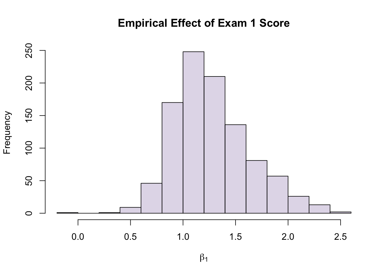
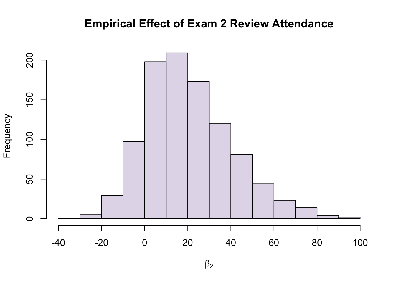
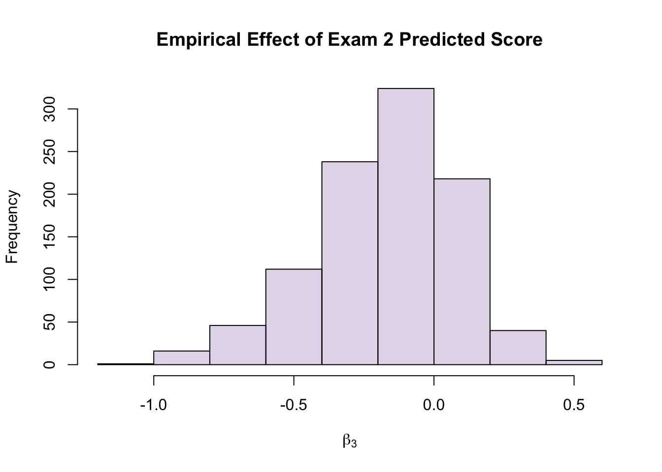
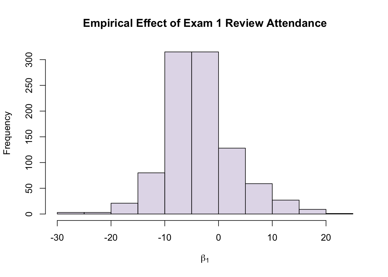
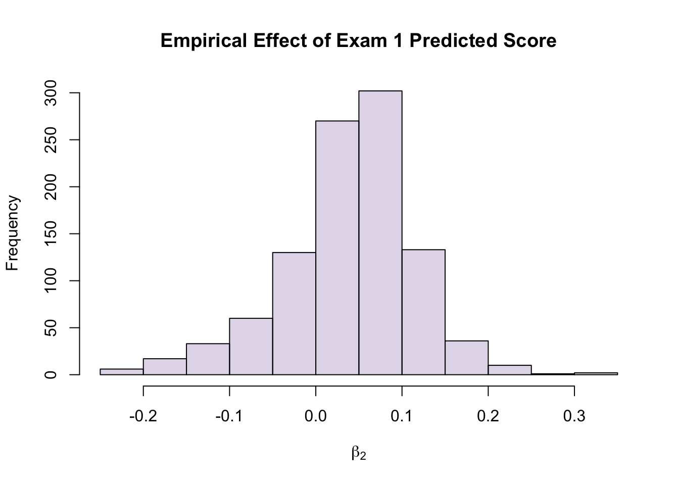
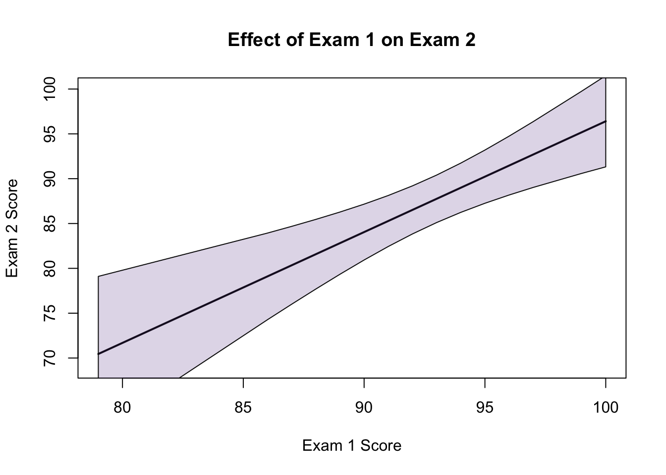
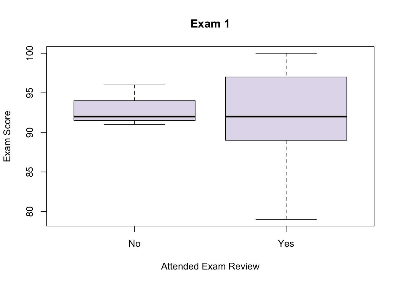
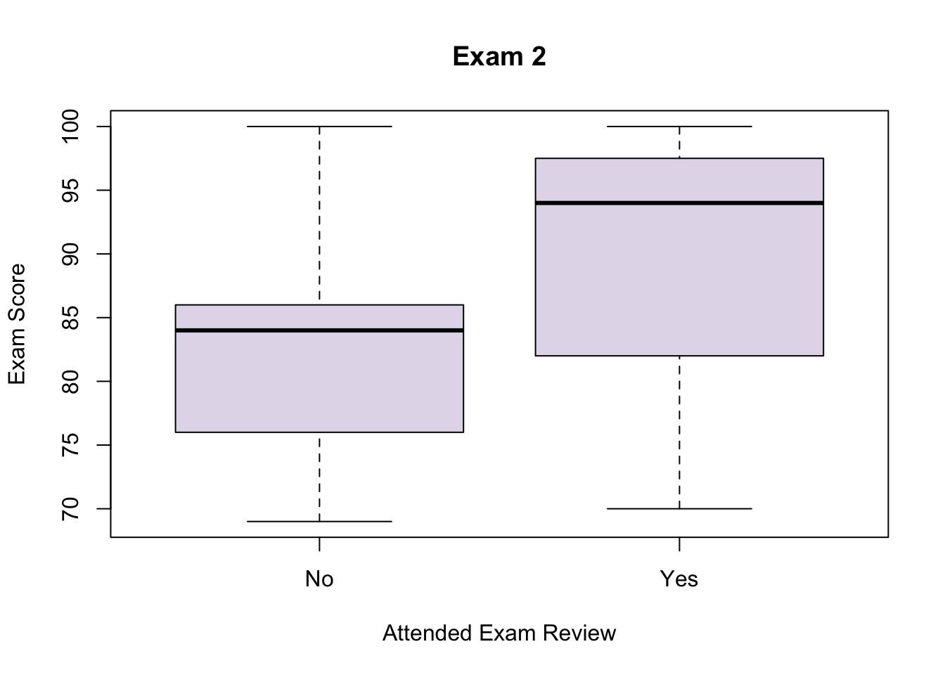
\[\hat{Y}=-29.4454581+1.2176886*E+16.5984930*A+-0.1239292*P\]
\(E \rightarrow\) Exam 1 Score
\(A \rightarrow\) 1 if you attended the Exam 2 review, 0 if you didn’t
\(P \rightarrow\) Predicted Exam 2 Score
Note: While the uncertainty on this formula is insane, it was trained with your data, so you MIGHT actually be able to recover your score from this.
Review
Hypothesis Testing for Population Mean:
- State the null and alternate hypotheses
- Choose a significance level \(\alpha =\) (allowed probability of Type I error).
- Compute the test statistic:
\[t = \frac{\bar{x} - \mu_0}{{s}/{\sqrt{n}}}\]
Since \(\sigma\) is unknown, we replace it with the sample standard deviation \(s\)
We use the \(t\) statistic, which comes from the \(t\) distribution with \(\text{df} = n - 1\)
- Compute the P-value of the test statistic \(t\).
Left-tailed test: \(P\)-value = area under the \(t\) distribution to the left of \(t\), i.e., \(P(T < t)\)
Right-tailed test: \(P\)-value = area under the \(t\) distribution to the right of \(t\), i.e., \(P(T > t)\)
Two-tailed test: \(P\)-value = sum of the areas under the \(t\) distribution to the left of \(-|t|\) and right of \(|t|\), i.e., \(2 * P(T < -|t|)\)
The degrees of freedom for the \(t\) distribution is \(\text{df} = n - 1\)
- Determine whether to reject \(H_0\):
Reject \(H_0\) if \(P\)-value \(\leq \alpha\)
Do not reject \(H_0\) if \(P\)-value \(> \alpha\)
- State a conclusion
Hypothesis Testing for Population Proportion:
Step 1: State the null and alternate hypotheses
The null hypothesis is of the form:
\[ H_0 : p = p_0 \]
The alternate hypothesis is in one of the three forms:
Left-tailed: \(H_1 : p < p_0\)
Right-tailed: \(H_1 : p > p_0\)
Two-tailed: \(H_1 : p \neq p_0\)
Step 2: Choose a significance level \(\alpha\)
Step 3: Compute the test statistic:
\[ z = \frac{\hat{p} - p_0}{\sqrt{\frac{p_0(1 - p_0)}{n}}} \]
Step 4: Compute the P-value of the test statistic \(z\)
Left-tailed: P-value = area under the standard normal distribution to the left of \(z\)
- i.e., \(P(Z < z)\)
Right-tailed: P-value = area under the standard normal distribution to the right of \(z\)
- i.e., \(P(Z > z)\)
Two-tailed: P-value = sum of the areas under the standard normal distribution to the left of \(-|z|\) and right of \(|z|\)
- i.e., \(2 * P(Z < -|z|)\)
Step 5: Determine whether to reject \(H_0\):
Reject \(H_0\) if P-value \(\leq \alpha\)
Do not reject \(H_0\) if P-value \(> \alpha\)
Step 6: State a conclusion
One-Sample Hypothesis Tests
Let’s look over some vocabulary:
Null Hypothesis \(H_0\)
The statement we are holding as known and established information
- i.e., The average body weight of an adult cat is \(10\) lbs.
\[H_0:\mu=10\]
Alternate Hypothesis \(H_a\) or \(H_1\)
The statement we are testing to determine the accuracy of
- I believe that the cats I interact with regularly have a different average body weight than the population
\[H_a:\mu \neq 10\]
Test Statistic \(t^*\)
A value calculated as part of the hypothesis testing process. We place it into a \(t\)-table (or \(z\)-table depending) to get a \(p\)-value.
\[t^* = \frac{\bar{x} - \mu_0}{{s}/{\sqrt{n}}}\]
- I weighed \(4\) of my friends cats and my own cat and found that their average body weight was \(8\) pounds, with a standard deviation of \(2.49\)
\[t^* = \frac{8 - 10}{{2.49}/{\sqrt{5}}}\]
\[t^*=-1.796039\]
A look at one of the participants in our study:

Significance level \(\alpha\)
The percentage probability we incur Type 1 Error in our hypothesis testing process
- I want to test my cat weight hypothesis at \(\alpha=0.05\)
P-value
The final statistic calculated in a hypothesis test, used to determine if we reject or fail to reject the null hypothesis
\[2*P(T>t^*)=0.15\]
\[0.15>\alpha \quad \text{Fail to Reject} \ H_0\]
Statistically Significant
We refer to a result as statistically significant if we tested it against a null hypothesis and proceeded to reject the null hypothesis
- There is insufficient evidence to suggest that the body weight of the cats that interact with regularly have a statistically significant difference in average body weight from the population
In-Class Exercises
Problem 1
Identify the following statements are true or false.
If \(P = 0.03\), the result is statistically significant at the \(\alpha = 0.05\) level
If \(P = 0.03\), the null hypothesis is rejected at the \(\alpha = 0.05\) level
If \(P = 0.03\), the result is statistically significant at the \(\alpha = 0.01\) level
If \(P = 0.03\), the null hypothesis is rejected at the \(\alpha = 0.01\) level
Problem 2
The average uptake of oxygen in the general adult population is 38.2 ml/kg. A sample of 40 joggers gave a sample mean of 40.5 ml/kg with a standard deviation of 6.0 ml/kg for oxygen uptake. A physician would like to know whether or not joggers have a significantly higher average oxygen uptake than the general population.
a. State the null and alternate hypotheses.
b. Compute the value of the test statistic.
c. Select the correct interval for the P-value.
- P-value \(\leq0.01\)
- \(0.01<\) P-value \(\leq0.025\)
- \(0.025<\) P-value \(\leq0.05\)
- P-value \(>0.05\)
d. Is \(H_0\) rejected at the \(\alpha=0.05\) level? Explain.
e. Based on your decision in (d), state a conclusion in the context of this problem.
Problem 3
The student president at Upper Midwest University has claimed that students living off-campus at UMU pay an average of $700 in rent per month. A reporter for the student newspaper believes this number is too high and decided to investigate.
The reporter took a random sample of 20 UMU students living off-campus and found that they pay an average monthly rent of $670. Assume rents at UMU are approximately normal with \(\sigma = 70\).
Test at the 5% significance level whether the mean monthly rent paid by off-campus UMU students is actually less than $700.
Problem 4
Generic drugs are lower-cost substitutes for brand-name drugs. Before a generic drug can be sold in the United States, it must be tested and found to perform equivalently to the brand-name product. The U.S. Food and Drug Administration is now supervising the testing of a new generic antifungal ointment. The brand-name ointment is known to deliver a mean of 3.5 micrograms of active ingredient to each square centimeter of skin.
As part of the testing, seven subjects apply the ointment. Six hours later, the amount of drug that has been absorbed into the skin is measured. The amounts, in micrograms, are:
\[2.6, \ 3.2, \ 2.1,\ 3.0,\ 3.1,\ 2.9,\ 3.7\]
How strong is the evidence that the mean amount absorbed differs from 3.5 micrograms? Use the \(\alpha=0.05\) level of significance.
Problem 4
A movie production company is releasing a movie with the hopes that many viewers will return to see the movie in the theater for a second time. Their target is to have more than 30% of the viewers want to see the movie again. They showed the movie to a test audience of 200 people and asked after the movie if the audience would see the movie in theaters again. Of the test audience, 68 people said they would see the movie again.
a. The production company would like to test if more than 30% of the viewers will return to see the movie. State the appropriate null and alternate hypotheses.
b. Compute the value of the test statistic.
c. Select the correct interval for the P-value.
- P-value \(\leq0.01\)
- \(0.01<\) P-value \(\leq0.025\)
- \(0.025<\) P-value \(\leq0.05\)
- P-value \(>0.05\)
d. Is \(H_0\) rejected at the \(\alpha=0.05\) level? Explain.
e. Based on your decision in (d), state a conclusion in the context of this problem.
- Go away